This document provides exercises related to inverse kinematics and manipulator kinematics. It includes exercises involving deriving inverse kinematics solutions for specific manipulator configurations, sketching workspaces, determining the number of inverse kinematics solutions, and programming inverse kinematics routines. It also provides sample manipulator configurations and forward kinematics equations to use in working through the exercises.

1. 128 Chapter 4 Inverse manipulator kinematics
is moderately expensive computationally, but the other solutions are found very
quickly by summing and differencing angles, subtracting jr, and so on.
BIBLIOGRAPHY
[1] B. Roth, J. Rastegar, and V. Scheinman, "On the Design of Computer Controlled
Manipulators," On the Theory and Practice of Robots and Manipulators, Vol. 1, First
CISM-IFToMM Symposium, September 1973, pp. 93—113.
[2] B. Roth, "Performance Evaluation of Manipulators from a Kinematic Viewpoint," Per-
formance Evaluation of Manipulators, National Bureau of Standards, special publication,
1975.
[3] D. Pieper and B. Roth, "The Kinematics of Manipulators Under Computer Control,"
Proceedings of the Second International Congress on Theory of Machines and Mechanisms,
Vol. 2, Zakopane, Poland, 1969, pp. 159—169.
[4] D. Pieper, "The Kinematics of Manipulators Under Computer Control," Unpublished
Ph.D. Thesis, Stanford University, 1968.
[5] R.P. Paul, B. Shimano, and G. Mayer, "Kinematic Control Equations for Simple Manip-
ulators," IEEE Transactions on Systems, Man, and Cybernetics, Vol. SMC-11, No. 6,
1981.
[6] L. Tsai and A. Morgan, "Solving the Kinematics of the Most General Six- and Five-
degree-of-freedom Manipulators by Continuation Methods," Paper 84-DET-20, ASME
Mechanisms Conference, Boston, October 7—10, 1984.
[7] C.S.G. Lee and M. Ziegler, "Geometric Approach in Solving Inverse Kinematics of
PUMA Robots," IEEE Transactions on Aerospace and Electronic Systems, Vol. AES-20,
No. 6, November 1984.
[8] W. Beyer, CRC Standard Mathematical Tables, 25th edition, CRC Press, Inc., Boca
Raton, FL, 1980.
[9] R. Burington, Handbook of Mathematical Tables and Formulas, 5th edition, McGraw-
Hill, New York, 1973.
[10] J. Hollerbach, "A Survey of Kinematic Calibration," in The Robotics Review, 0. Khatib,
J. Craig, and T. Lozano-Perez, Editors, MIT Press, Cambridge, MA, 1989.
[II] Y. Nakamura and H. Hanafusa, "Inverse Kinematic Solutions with Singularity Robust-
ness for Robot Manipulator Control," ASME Journal of Dynamic Systems, Measurement,
and Control, Vol. 108, 1986.
[12] D. Baker and C. Wampler, "On the Inverse Kinematics of Redundant Manipulators,"
International Journal of Robotics Research, Vol. 7, No. 2, 1988.
[13] L.W. Tsai, Robot Analysis: The Mechanics of Serial and Parallel Manipulators, Wiley,
New York, 1999.
EXERCISES
4.1 [15] Sketch the fingertip workspace of the three-link manipulator of Chapter 3,
Exercise 3.3 for the case = 15.0, 12 = 10.0, and 13 = 3.0.
4.2 [26] Derive the inverse kinematics of the three-link manipulator of Chapter 3,
Exercise 3.3.
4.3 [12] Sketch the fingertip workspace of the 3-DOF manipulator of Chapter 3,
Example 3.4.

2. Exercises 129
4.4 [24] Derive the inverse kinematics of the 3-DOF manipulator of Chapter 3,
Example 3.4.
4.5 [38] Write a Pascal (or C) subroutine that computes all possible solutions for the
PUMA 560 manipulator that lie within the following joint limits:
—170.0 <170.0,
—225.0 <45.0,
—250.0 <63 <75.0,
—135.0 <64 <135.0,
—100.0 <95 <100.0,
—180.0 <°6 <180.0.
Use the equations derived in Section 4.7 with these numerical values (in inches):
a2 = 17.0,
£13 = 0.8,
d3 = 4.9,
d4 = 17.0.
4.6 [15] Describe a simple algorithm for choosing the nearest solution from a set of
possible solutions.
4.7 [10] Make a list of factors that might affect the repeatability of a manipulator.
Make a second list of additional factors that affect the accuracy of a manipulator.
4.8 [12] Given a desired position and orientation of the hand of a three-link planar
rotary-jointed manipulator, there are two possible solutions. If we add one more
rotational joint (in such a way that the arm is still planar), how many solutions
are there?
4.9 [26] Figure 4.13 shows a two-link planar arm with rotary joints. For this arm, the
second link is half as long as the first—that is, ii = 212. The joint range limits in
FIGURE 4.13: Two-link planar manipulator.
L1

3. 130 Chapter 4 Inverse manipulator kinematics
degrees are
0 <180,
—90 <180.
Sketch the approximate reachable workspace (an area) of the tip of link 2.
4.10 [23] Give an expression for the subspace of the manipulator of Chapter 3,
Example 3.4.
4.11 [24] A 2-DOF positioning table is used to orient parts for arc-welding. The
forward kinematics that locate the bed of the table (link 2) with respect to the
base (link 0) are
r c1c2 —c1s2 s1 12s1 +
OT_I S2 C2 0 0
2
—
s1s2 c1 12c1 + h1
LO 0 0 1
Given any unit direction fixed in the frame of the bed (link 2), give the
inverse-kinematic solution for 02 such that this vector is aligned with 02 (i.e.,
upward). Are there multiple solutions? Is there a singular condition for which a
unique solution cannot be obtained?
4.12 [22] In Fig. 4.14, two 3R mechanisms are pictured. In both cases, the three axes
intersect at a point (and, over all configurations, this point remains fixed in space).
The mechanism in Fig. 4.14(a) has link twists (as) of magnitude 90 degrees. The
mechanism in Fig. 4.14(b) has one twist of in magnitude and the other of 180—
in magnitude.
The mechanism in Fig. 4.14(a) can be seen to be in correspondence with Z—Y—Z
Euler angles, and therefore we know that it suffices to orient link 3 (with arrow
in figure) arbitrarily with respect to the link 0. Because 0 is not equal to 90
degrees, it turns out that the other mechanism cannot orient link 3 arbitrarily.
FIGURE 4.14: Two 3R mechanisms (Exercise 4.12).
(a) (b)

4. zo,1
Exercises 131
FIGURE 4.15: A 4R manipulator shown in the position e = [0,900, —90°, 01T (Exer-
cise 4.16).
Describe the set of orientations that are unattainable with the second mechanism.
Note that we assume that all joints can turn 360 degrees (i.e. no limits) and we
assume that the links may pass through each other if need be (i.e., workspace not
limited by self-coffisions).
4.13 [13] Name two reasons for which closed-form analytic kinematic solutions are
preferred over iterative solutions.
4.14 [14] There exist 6-DOF robots for which the kinematics are NOT closed-form
solvable. Does there exist any 3-DOF robot for which the (position) kinematics
are NOT closed-form solvable?
4.15 [38] Write a subroutine that solves quartic equations in closed form. (See [8, 9].)
4.16 [25] A 4R manipulator is shown schematically in Fig. 4.15. The nonzero link
parameters are a1 = 1, a2 = 45°, d3 = and a3 = and the mechanism is
pictured in the configuration corresponding to e = [0,90°, —90°, 0]T. Each joint
has ±180° as limits. Find all values of 83 such that
= [1.1, 1.5,
4.17 [25] A 4R manipulator is shown schematically in Fig. 4.16. The nonzero link
parameters are a1 = —90°, d2 = 1, a2 = 45°, d3 = 1, and a3 = 1, and the
mechanism is pictured in the configuration corresponding to 0 = [0, 0, 90°, 0]T.
Each joint has ±180° as limits. Find all values of 83 such that
= [0.0, 1.0, 1414]T
4.18 [15] Consider the RRP manipulator shown in Fig. 3.37. How many solutions do
the (position) kinematic equations possess?
4.19 [15] Consider the RRR manipulator shown in Fig. 3.38. How many solutions do
the (position) kinematic equations possess?
4.20 [15] Consider the R PP manipulator shown in Fig. 3.39. How many solutions do
the (position) kinematic equations possess?
I
I
I
I
1
I
I
I
I
xo,1 y-)
A
x4

5. 132 Chapter 4 Inverse manipulator kinematics
FIGURE 4.16: A 4R manipulator shown in the position 0 = [0,0, 900, 0]T (Exer-
cise 4.17).
4.21 [15] Consider the PRR manipulator shown in Fig. 3.40. How many solutions do
the (position) kinematic equations possess?
4.22 [15] Consider the PPP manipulator shown in Fig. 3.41. How many solutions do
the (position) kinematic equations possess?
4.23 [38] The following kinematic equations arise in a certain problem:
sine —asin9+b,
= ccos9 +d,
Given a, b, c, d, and i/i, show that, in the general case, there are four solutions for
6. Give a special condition under which there are just two solutions for 9.
4.24 [20] Given the description of link frame {i} in terms of link frame {i — 1), find the
four Denavit—Hartenberg parameters as functions of the elements of Y'T.
PROGRAMMING EXERCISE (PART 4)
1. Write a subroutine to calculate the inverse kinematics for the three-link manipu-
lator of Section 4.4. The routine should pass arguments in the form
Procedure INVKIN(VAR wreib: frame; VAR current, near, far: vec3;
VAR sol: boolean);
where "wreib," an input, is the wrist frame specified relative to the base frame;
"current," an input, is the current position of the robot (given as a vector of joint
angles); "near" is the nearest solution; "far" is the second solution; and "sol" is
a flag that indicates whether solutions were found. (sol = FALSE if no solutions
were found). The link lengths (meters) are
11 = 17 = 0.5.
zo,1
L/
yo,1
x4

6. MATLAB Exercise 4 133
The joint ranges of motion are
—170° 170°.
Test your routine by calling it back-to-back with KIN to demonstrate that they are
indeed inverses of one another.
2. A tool is attached to link 3 of the manipulator. This tool is described by the
tool frame relative to the wrist frame. Also, a user has described his work area, the
station frame relative to the base of the robot, as T. Write the subroutine
Procedure SOLVE(VAR -brels: frame; VAR current, near, far: vec3;
VAR sol: boolean);
where "trels" is the {T} frame specified relative to the {S} frame. Other parameters
are exactly as in the INVKIN subroutine. The defmitions of {T} and {S} should be
globally defined variables or constants. SOLVE should use calls to TMULT, TINVERT,
and INVKIN.
3. Write a main program that accepts a goal frame specified in terms of x, y, and
This goal specification is (T} relative to {S}, which is the way the user wants to
specify goals.
The robot is using the same tool in the same working area as in Programming
Exercise (Part 2), so {T} and {S} are defined as
= [x y 9] = [0.1 0.2 30.0],
= [x y 8] = [—0.1 0.3 0.0].
Calculate the joint angles for each of the following three goal frames:
[x1 Yi = [0.0 0.0 — 90.0],
Er7 Y2 02] = [0.6 —0.3 45.0],
[x3 Y3 03] = [—0.4 0.3 120.0],
[x4 04] = [0.8 1.4 30.0].
Assume that the robot wifi start with all angles equal to 0.0 and move to these
three goals in sequence. The program should find the nearest solution with respect
to the previous goal point. You should call SOLVE and WHERE back-to-back to make
sure they are truly inverse functions.
MATLAB EXERCISE 4
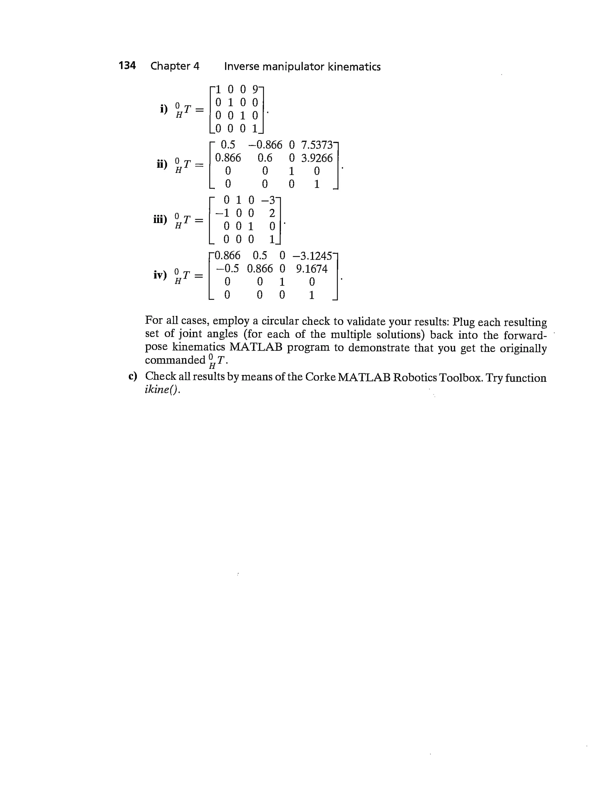
This exercise focuses on the inverse-pose kinematics solution for the planar 3-DOF,
3R robot. (See Figures 3.6 and 3.7; the DH parameters are given in Figure 3.8.) The
following fixed-length parameters are given: L1 = 4, L2 = 3, and L3 = 2(m).
a) Analytically derive, by hand, the inverse-pose solution for this robot: Given
T, calculate all possible multiple solutions for 8-, 83 }. (Three methods are
presented in the text—choose one of these.) Hint: To simplify the equations, first
calculate from and L3.
b) Develop a MATLAB program to solve this planar 3R robot inverse-pose kine-
matics problem completely (i.e., to give all multiple solutions). Test your program,
using the following input cases:

7. 134 Chapter 4 Inverse manipulator kinematics
1009
' 0100
H — 0 0 1 0
0001
0.5 —0.866 0 7.5373
o 0.866 0.6 0 3.9266
0 0 1 0
0 0 01
0 1 0 —3
o — —100 2
I1I)HT_ 001 0
000 1
rO.866 0.5 0 —3.1245
o I —0.5 0.866 0 9.1674
0 0 1 0
Lo 0 0 1
For all cases, employ a circular check to validate your results: Plug each resulting
set of joint angles (for each of the multiple solutions) back into the forward-
pose kinematics MATLAB program to demonstrate that you get the originally
commanded
c) Check all results by means of the Corke MATLAB Robotics Toolbox. Try function
ikineQ.