SlideShare a Scribd company logo
2
Chapter
Representing Position
and Orientation
Fig. 2.1.
a The point P is described by a co-
ordinate vector with respect to an
absolute coordinate frame. b The
points are described with respect
to the object’s coordinate frame {B}
which in turn is described by a
relative pose ξB.Axes are deno-
ted by thick lines with an open
arrow, vectors by thin lines with a
swept arrow head and a pose by a
thick line with a solid head
Fig. 2.2.
The point P can be described by
coordinate vectors relative to
either frame {A} or {B}. The pose
of {B} relative to {A} is AξB
A fundamental requirement in robotics and computer vision is to represent
the position and orientation of objects in an environment. Such objects in-
clude robots, cameras, workpieces, obstacles and paths.
A point in space is a familiar concept from mathematics and can be de-
scribed by a coordinate vector, also known as a bound vector, as shown in
Fig. 2.1a. The vector represents the displacement of the point with respect
to some reference coordinate frame.A coordinate frame, or Cartesian coor-
dinate system, is a set of orthogonal axes which intersect at a point known
as the origin.
More frequently we need to consider a set of points that comprise some
object. We assume that the object is rigid and that its constituent points
maintain a constant relative position with respect to the object’s coordinate
frame as shown in Fig. 2.1b. Instead of describing the individual points we
describe the position and orientation of the object by the position and ori-
entation of its coordinate frame. A coordinate frame is labelled, {B} in this
case, and its axis labels xB and yB adopt the frame’s label as their subscript.
The position and orientation of a coordinate frame is known as its pose
and is shown graphically as a set of coordinate axes. The relative pose of a
framewithrespecttoareferencecoordinateframeisdenotedbythesymbol ξ
16
– pronounced ksi. Figure 2.2 shows two frames {A} and {B} and the relative pose AξB
which describes {B} with respect to {A}. The leading superscript denotes the reference
coordinate frame and the subscript denotes the frame being described. We could also
think of AξB as describing some motion – imagine picking up {A} and applying a dis-
placement and a rotation so that it is transformed to {B}.If the initial superscript is miss-
ingweassumethatthechangeinposeisrelativetotheworldcoordinateframedenoted O.
The point P in Fig. 2.2 can be described with respect to either coordinate frame.
Formally we express this as
(2.1)
where the right-hand side expresses the motion from {A} to {B} and then to P. The
operator · transforms the vector, resulting in a new vector that describes the same
point but with respect to a different coordinate frame.
An important characteristic of relative poses is that they can be composed or com-
pounded. Consider the case shown in Fig. 2.3. If one frame can be described in terms
of another by a relative pose then they can be applied sequentially
which says,in words,that the pose of {C} relative to {A} can be obtained by compound-
ing the relative poses from {A} to {B} and {B} to {C}.We use the operator ⊕ to indicate
composition of relative poses.
For this case the point P can be described
Later in this chapter we will convert these abstract notions of ξ, · and ⊕ into stan-
dard mathematical objects and operators that we can implement in MATLAB®.
In the examples so far we have shown 2-dimensional coordinate frames. This is
appropriate for a large class of robotics problems,particularly for mobile robots which
operate in a planar world. For other problems we require 3-dimensional coordinate
frames to describe objects in our 3-dimensional world such as the pose of a flying or
underwater robot or the end of a tool carried by a robot arm.
Fig. 2.3.
The point P can be described by
coordinate vectors relative to
either frame {A}, {B} or {C}. The
frames are described by relative
poses
In relative pose composition we can check that we have our reference frames correct by ensuring
that the subscript and superscript on each side of the ⊕ operator are matched.We can then cancel
out the intermediate subscripts and superscripts
leaving just the end most subscript and superscript which are shown circled.
Chapter 2 · Representing Position and Orientation
17
Figure 2.4 shows a more complex 3-dimensional example in a graphical form where
we have attached 3D coordinate frames to the various entities and indicated some rela-
tive poses. The fixed camera observes the object from its fixed viewpoint and estimates
the object’s pose relative to itself.The other camera is not fixed,it is attached to the robot
at some constant relative pose and estimates the object’s pose relative to itself.
An alternative representation of the spatial relationships is a directed graph (see
Appendix J) which is shown in Fig. 2.5. Each node in the graph represents a pose and
each edge represents a relative pose.An arrow from X to Y is denoted X
ξY and describes
the pose of Y relative to X. Recalling that we can compose relative poses using the
⊕ operator we can write some spatial relationships
and each equation represents a loop in the graph. Each side of the equation represents
a path through the network, a sequence of edges (arrows) that are written in head to
tail order. Both sides of the equation start and end at the same node.
A very useful property of poses is the ability to perform algebra. The second loop
equation says, in words, that the pose of the robot is the same as composing two rela-
tive poses: from the world frame to the fixed camera and from the fixed camera to the
Fig. 2.4.
Multiple 3-dimensional coordi-
nate frames and relative poses
René Descartes (1596–1650) was a French philosopher,mathematician and part-time mercenary.
He is famous for the philosophical statement “Cogito, ergo sum” or “I am thinking, therefore I
exist”or“I think, therefore I am”. He was a sickly child and developed a life-long habit of lying in
bed and thinking until late morning. A possibly apocryphal story is that during one such morn-
ing he was watching a fly walk across the ceiling and realized that he could describe its position in
terms of its distance from the two edges of the ceiling. This coordinate system, the Cartesian
system, forms the basis of modern (analytic) geometry and influenced the development of mod-
ern calculus. In Sweden at the invitation of Queen Christine he was obliged to rise at 5 a.m.,
breaking his lifetime habit – he caught pneumonia and died. His remains were later moved to
Paris, and then moved several times, and there is now some debate about where his remains are.
After his death, the Roman Catholic Church placed his works on the Index of Prohibited Books.
Chapter 2 · Representing Position and Orientation
In mathematical objects terms poses
constituteagroup–asetofobjectsthat
supports an associative binary operator
(composition) whose result belongs to
the group, an inverse operation and an
identity element.In this case the group
is the special Euclidean group in either
2 or 3 dimensions which are commonly
referred to as SE(2) or SE(3) respectively.
18
robot. We can subtract ξF from both sides of the equation by adding the inverse of ξF
which we denote as ξF and this gives
which is the pose of the robot relative to the fixed camera.
Fig. 2.5.
Spatial example of Fig. 2.4
expressed as a directed graph
There are just a few algebraic rules:
where 0 represents a zero relative pose. A pose has an inverse
which is represented graphically by an arrow from Y to X.Relative poses can also
be composed or compounded
It is important to note that the algebraic rules for poses are different to nor-
mal algebra and that composition is not commutative
with the exception being the case where ξ1 ⊕ ξ2 = 0.A relative pose can transform a
point expressed as a vector relative to one frame to a vector relative to another
So what is ξ? It can be any mathematical object that supports the algebra described
above and is suited to the problem at hand. It will depend on whether we are consider-
ing a 2- or 3-dimensional problem. Some of the objects that we will discuss in the rest
of this chapter include vectors as well as more exotic mathematical objects such as
homogeneous transformations, orthonormal rotation matrices and quaternions. For-
tunately all these mathematical objects are well suited to the mathematical program-
ming environment of MATLAB®.
Chapter 2 · Representing Position and Orientation
19
To recap:
1. A point is described by a coordinate vector that represents its displacement from a
reference coordinate system;
2. A set of points that represent a rigid object can be described by a single coordinate
frame,and its constituent points are described by displacements from that coordinate
frame;
3. The position and orientation of an object’s coordinate frame is referred to as its
pose;
4. A relative pose describes the pose of one coordinate frame with respect to another
and is denoted by an algebraic variable ξ;
5. A coordinate vector describing a point can be represented with respect to a different
coordinate frame by applying the relative pose to the vector using the · operator;
6. We can perform algebraic manipulation of expressions written in terms of relative
poses.
The remainder of this chapter discusses concrete representations of ξ for various
common cases that we will encounter in robotics and computer vision.
2.1 lRepresenting Pose in 2-Dimensions
A 2-dimensional world, or plane, is familiar to us from high-school Euclidean geom-
etry. We use a Cartesian coordinate system or coordinate frame with orthogonal axes
denoted x and y and typically drawn with the x-axis horizontal and the y-axis vertical.
The point of intersection is called the origin. Unit-vectors parallel to the axes are de-
noted ' and (. A point is represented by its x- and y-coordinates (x, y) or as a bound
vector
(2.2)
Figure 2.6 shows a coordinate frame {B} that we wish to describe with respect to the
reference frame {A}.We can see clearly that the origin of {B} has been displaced by the
vector t = (x, y) and then rotated counter-clockwise by an angle θ. A concrete repre-
sentation of pose is therefore the 3-vector AξB ∼ (x, y, θ), and we use the symbol ∼ to
denote that the two representations are equivalent. Unfortunately this representation
is not convenient for compounding since
is a complex trigonometric function of both poses. Instead we will use a different way
of representing rotation.
The approach is to consider an arbitrary point P with respect to each of the coordi-
nate frames and to determine the relationship between Ap and Bp. Referring again to
Fig. 2.6 we will consider the problem in two parts: rotation and then translation.
Euclid of Alexandria (ca. 325 bce–265 bce) was an Egyptian mathematician who is considered
the “father of geometry”. His book Elements deduces the properties of geometrical objects and
integers from a small set of axioms.
Elements is probably the most successful book in the history of mathematics.It describes plane
geometry and is the basis for most people’s first introduction to geometry and formal proof, and
is the basis of what we now call Euclidean geometry. Euclidean distance is simply the distance
between two points on a plane. Euclid also wrote Optics which describes geometric vision and
perspective.
2.1 · Representing Pose in 2-Dimensions
20
To consider just rotation we create a new frame {V} whose axes are parallel to those of
{A} but whose origin is the same as {B}, see Fig. 2.7.According to Eq. 2.2 we can express
the point P with respect to {V} in terms of the unit-vectors that define the axes of the frame
(2.3)
which we have written as the product of a row and a column vector.
The coordinate frame {B} is completely described by its two orthogonal axes which
we represent by two unit vectors
which can be written in matrix form as
(2.4)
Using Eq. 2.2 we can represent the point P with respect to {B} as
and substituting Eq. 2.4 we write
(2.5)
Now by equating the coefficients of the right-hand sides of Eq. 2.3 and Eq. 2.5 we
write
which describes how points are transformed from frame {B} to frame {V} when the
frame is rotated. This type of matrix is known as a rotation matrix and denoted V
RB
(2.6)
Fig. 2.6.
Two 2D coordinate frames {A}
and {B} and a world point P.
{B} is rotated and translated
with respect to {A}
Chapter 2 · Representing Position and Orientation
21
The rotation matrix VRB has some special properties. Firstly it is orthonormal
(also called orthogonal) since each of its columns is a unit vector and the columns are
orthogonal. In fact the columns are simply the unit vectors that define {B} with re-
spect to {V} and are by definition both unit-length and orthogonal.
Secondly,its determinant is +1,which means that R belongs to the special orthogo-
nal group of dimension 2 or R ∈ SO(2) ⊂ R2×2. The unit determinant means that the
length of a vector is unchanged after transformation, that is, |Bp| = |Vp|, ∀θ.
Orthonormal matrices have the very convenient property that R−1 = RT, that is, the
inverse is the same as the transpose. We can therefore rearrange Eq. 2.6 as
Note that inverting the matrix is the same as swapping the superscript and subscript,
which leads to the identity R(−θ) = R(θ )T
.
It is interesting to observe that instead of representing an angle, which is a scalar,
we have used a 2 × 2 matrix that comprises four elements, however these elements
are not independent. Each column has a unit magnitude which provides two con-
straints. The columns are orthogonal which provides another constraint. Four ele-
ments and three constraints are effectively one independent value. The rotation ma-
trix is an example of a non-minimum representation and the disadvantages such as
the increased memory it requires are outweighed, as we shall see, by its advantages
such as composability.
The second part of representing pose is to account for the translation between the
origins of the frames shown in Fig. 2.6. Since the axes {V} and {A} are parallel this is
simply vectorial addition
(2.7)
(2.8)
(2.9)
or more compactly as
(2.10)
Fig. 2.7.
Rotated coordinate frames in 2D.
The point P can be considered
with respect to the red or blue
coordinate frame
2.1 · Representing Pose in 2-Dimensions
See Appendix D which provides a re-
fresher on vectors, matrices and linear
algebra.
22
where t = (x, y) is the translation of the frame and the orientation is ARB. Note that
ARB = TRB since the axes of {A} and {V} are parallel.The coordinate vectors for point P
are now expressed in homogenous form and we write
and ATB is referred to as a homogeneous transformation. The matrix has a very
specific structure and belongs to the special Euclidean group of dimension 2 or
T ∈ SE(2) ⊂ R3×3.
By comparison with Eq. 2.1 it is clear that ATB represents relative pose
A vector (x, y) is written in homogeneous form as p ∈ P2
, p = (x1, x2, x3) where x = x1/x3,y = x2/x3
and x3 ≠ 0. The dimension has been increased by one and a point on a plane is now represented
by a 3-vector. To convert a point to homogeneous form we typically append a one p = (x, y, 1).
The tilde indicates the vector is homogeneous.
Homogeneous vectors have the important property that p is equivalent to λp, ∀λ ≠ 0 which
we write as p λp. That is p represents the same point in the plane irrespective of the overall
scaling factor. Homogeneous representation is important for computer vision that we discuss in
Part IV. Additional details are provided in Appendix I.
A concrete representation of relative pose ξ is ξ ∼ T ∈ SE(2) and T1 ⊕ T2 T1T2
which is standard matrix multiplication.
One of the algebraic rules from page 18 is ξ ⊕ 0 = ξ. For matrices we know
that TI = T, where I is the identify matrix, so for pose 0 I the identity matrix.
Another rule was that ξ ξ = 0. We know for matrices that TT−1 = I which im-
plies that T T−1
For a point p ∈ P2 then T·p Tp which is a standard matrix-vector product.
To make this more tangible we will show some numerical examples using MATLAB®
and the Toolbox. We create a homogeneous transformation using the function se2
>> T1 = se2(1, 2, 30*pi/180)
T1 =
0.8660 -0.5000 1.0000
0.5000 0.8660 2.0000
0 0 1.0000
which represents a translation of (1, 2) and a rotation of 30°. We can plot this, relative
to the world coordinate frame, by
Chapter 2 · Representing Position and Orientation
23
>> axis([0 5 0 5]);
>> trplot2(T1, 'frame', '1', 'color', 'b')
The options specify that the label for the frame is {1} and it is colored blue and this
is shown in Fig. 2.8. We create another relative pose which is a displacement of (2, 1)
and zero rotation
>> T2 = se2(2, 1, 0)
T2 =
1 0 2
0 1 1
0 0 1
which we plot in red
>> hold on
>> trplot2(T2, 'frame', '2', 'color', 'r');
Now we can compose the two relative poses
>> T3 = T1*T2
T3 =
0.8660 -0.5000 2.2321
0.5000 0.8660 3.8660
0 0 1.0000
and plot it, in green, as
>> trplot2(T3, 'frame', '3', 'color', 'g');
We see that the displacement of (2, 1) has been applied with respect to frame {1}. It is
important to note that our final displacement is not (3, 3) because the displacement is
with respect to the rotated coordinate frame. The non-commutativity of composition
is clearly demonstrated by
>> T4 = T2*T1;
>> trplot2(T4, 'frame', '4', 'color', 'c');
and we see that frame {4} is different to frame {3}.
Now we define a point (3, 2) relative to the world frame
>> P = [3 ; 2 ];
which is a column vector and add it to the plot
>> plot_point(P, '*');
Fig. 2.8.
Coordinate frames drawn using
the Toolbox function trplot2
2.1 · Representing Pose in 2-Dimensions
24
To determine the coordinate of the point with respect to {1} we use Eq. 2.1 and
write down
and then rearrange as
Substituting numerical values
>> P1 = inv(T1) * [P; 1]
P1 =
1.7321
-1.0000
1.0000
where we first converted the Euclidean point to homogeneous form by appending a
one. The result is also in homogeneous form and has a negative y-coordinate in
frame {1}. Using the Toolbox we could also have expressed this as
>> h2e( inv(T1) * e2h(P) )
ans =
1.7321
-1.0000
where the result is in Euclidean coordinates.The helper function e2h converts Euclid-
ean coordinates to homogeneous and h2e performs the inverse conversion.More com-
pactly this can be written as
>> homtrans( inv(T1), P)
ans =
1.7321
-1.0000
The same point with respect to {2} is
>> P2 = homtrans( inv(T2), P)
P2 =
1
1
2.2 lRepresenting Pose in 3-Dimensions
The 3-dimensional case is an extension of the 2-dimensional case discussed in the
previous section. We add an extra coordinate axis, typically denoted by z, that is or-
thogonal to both the x- and y-axes. The direction of the z-axis obeys the right-hand
rule and forms a right-handed coordinate frame. Unit vectors parallel to the axes are
denoted ', ( and ) such that
(2.11)
A point P is represented by its x-, y- and z-coordinates (x, y, z) or as a bound vector
Figure 2.9 shows a coordinate frame {B} that we wish to describe with respect to the
reference frame {A}.We can see clearly that the origin of {B} has been displaced by the
vector t = (x, y, z) and then rotated in some complex fashion. Just as for the 2-dimen-
sional case the way we represent orientation is very important.
Chapter 2 · Representing Position and Orientation
In all these identities, the symbols from
left to right (across the equals sign) are a
cyclic permutation of the sequence xyz.
25
Our approach is to again consider an arbitrary point P with respect to each of
the coordinate frames and to determine the relationship between Ap and Bp. We will
again consider the problem in two parts: rotation and then translation. Rotation
is surprisingly complex for the 3-dimensional case and we devote all of the next sec-
tion to it.
2.2.1 lRepresenting Orientation in 3-Dimensions
Any two independent orthonormal coordinate frames
can be related by a sequence of rotations (not more than three)
about coordinate axes, where no two successive rotations may be about the same axis.
Euler’s rotation theorem (Kuipers 1999).
Figure 2.9 showed a pair of right-handed coordinate frames with very different orien-
tations, and we would like some way to describe the orientation of one with respect to
the other. We can imagine picking up frame {A} in our hand and rotating it until it
looked just like frame {B}. Euler’s rotation theorem states that any rotation can be con-
sidered as a sequence of rotations about different coordinate axes.
We start by considering rotation about a single coordinate axis.Figure 2.10 shows a
right-handed coordinate frame, and that same frame after it has been rotated by vari-
ous angles about different coordinate axes.
The issue of rotation has some subtleties which are illustrated in Fig. 2.11. This
shows a sequence of two rotations applied in different orders. We see that the final
orientation depends on the order in which the rotations are applied.This is a deep and
confounding characteristic of the 3-dimensional world which has intrigued mathema-
ticians for a long time. The implication for the pose algebra we have used in this chap-
ter is that the ⊕ operator is not commutative – the order in which rotations are applied
is very important.
Mathematicians have developed many ways to represent rotation and we will dis-
cuss several of them in the remainder of this section: orthonormal rotation matrices,
Euler and Cardan angles, rotation axis and angle, and unit quaternions. All can be
represented as vectors or matrices, the natural datatypes of MATLAB® or as a Toolbox
defined class. The Toolbox provides many function to convert between these repre-
sentations and this is shown diagrammatically in Fig. 2.15.
Fig. 2.9.
Two 3D coordinate frames {A}
and {B}. {B} is rotated and
translated with respect to {A}
Right-handrule. A right-handed coordinate frame is defined by the first three fingers of your right
hand which indicate the relative directions of the x-, y- and z-axes respectively.
2.2 · Representing Pose in 3-Dimensions
26
Rotation about a vector. Wrap your right hand around the vector with your thumb (your x-finger)
in the direction of the arrow. The curl of your fingers indicates the direction of increasing angle.
Fig. 2.10.
Rotation of a 3D coordinate
frame. a The original coordinate
frame, b–f frame a after various
rotations as indicated
Fig. 2.11.
Example showing the non-com-
mutivity of rotation. In the top
row the coordinate frame is rota-
ted by ü about the x-axis and
then ü about the y-axis. In the
bottom row the order of rota-
tions has been reversed. The
results are clearly different
Chapter 2 · Representing Position and Orientation
27
2.2.1.1 lOrthonormal Rotation Matrix
Just as for the 2-dimensional case we can represent the orientation of a coordinate
frame by its unit vectors expressed in terms of the reference coordinate frame. Each
unit vector has three elements and they form the columns of a 3 × 3 orthonormal
matrix ARB
(2.12)
which rotates a vector defined with respect to frame {B} to a vector with respect to {A}.
Thematrix Rbelongstothespecialorthogonalgroupof dimension 3orR ∈ SO(3) ⊂ R3×3.
It has the properties of an orthonormal matrix that were mentioned on page 16 such as
RT
= R−1
and det(R) = 1.
The orthonormal rotation matrices for rotation of θ about the x-, y- and z-axes are
The Toolbox provides functions to compute these elementary rotation matrices,for
example Rx(θ ) is
>> R = rotx(pi/2)
R =
1.0000 0 0
0 0.0000 -1.0000
0 1.0000 0.0000
Such a rotation is also shown graphically in Fig. 2.10b. The functions roty and rotz
compute Ry(θ ) and Rz(θ ) respectively.
The corresponding coordinate frame can be displayed graphically
>> trplot(R)
which is shown in Fig. 2.12a. We can visualize a rotation more powerfully using the
Toolbox function tranimate which animates a rotation
>> tranimate(R)
showing the world frame rotating into the specified coordinate frame.
2.2 · Representing Pose in 3-Dimensions
Reading the columns of an orthonormal rotation matrix from left to right tells us the directions
of the new frame’s axes in terms of the current coordinate frame. For example if
R =
1.0000 0 0
0 0.0000 -1.0000
0 1.0000 0.0000
the new frame has its x-axis in the old x-direction (1, 0, 0),its y-axis in the old z-direction (0, 0, 1),
and the new z-axis in the old negative y-direction (0, −1, 0).In this case the x-axis was unchanged
since this is the axis around which the rotation occurred.
28
To illustrate compounding of rotations we will rotate the frame of Fig. 2.12a again,
this time around its y-axis
>> rotx(pi/2) * roty(pi/2)
ans =
0.0000 0 1.0000
1.0000 0.0000 -0.0000
-0.0000 1.0000 0.0000
>> trplot(R)
to give the frame shown in Fig. 2.12b. In this frame the x-axis now points in the direc-
tion of the world y-axis.
The non-commutativity of rotation can be shown by reversing the order of the
rotations above
>> roty(pi/2)*rotx(pi/2)
ans =
0.0000 1.0000 0.0000
0 0.0000 -1.0000
-1.0000 0.0000 0.0000
which has a very different value.
We recall that Euler’s rotation theorem states that any rotation can be represented
by not more than three rotations about coordinate axes. This means that in general an
arbitrary rotation between frames can be decomposed into a sequence of three rota-
tion angles and associated rotation axes – this is discussed in the next section.
The orthonormal matrix has nine elements but they are not independent. The col-
umns have unit magnitude which provides three constraints.The columns are orthogo-
nal to each other which provides another three constraints. Nine elements and six
constraints is effectively three independent values.
2.2.1.2 lThree-Angle Representations
Euler’s rotation theorem requires successive rotation about three axes such that no
two successive rotations are about the same axis. There are two classes of rotation
sequence: Eulerian and Cardanian, named after Euler and Cardano respectively.
The Eulerian type involves repetition, but not successive, of rotations about one
particular axis: XYX, XZX, YXY, YZY, ZXZ, or ZYZ. The Cardanian type is character-
ized by rotations about all three axes: XYZ, XZY, YZX,YXZ, ZXY, or ZYX. In common
usage all these sequences are called Euler angles and there are a total of twelve to
choose from.
Fig. 2.12.
Coordinate frames displayed
using trplot. a Reference
frame rotated by ü about the
x-axis, b frame a rotated by ü
about the y-axis
Chapter 2 · Representing Position and Orientation
If the column vectors are ci , i ∈ 1 3
then c1 · c2 = c2 · c3 = c3 · c1 = 0.
29
It is common practice to refer to all 3-angle representations as Euler angles but this
is underspecified since there are twelve different types to choose from.The par-
ticularanglesequenceisoftenaconventionwithinaparticulartechnologicalfield.
The ZYZ sequence
(2.13)
is commonly used in aeronautics and mechanical dynamics,and is used in the Toolbox.
The Euler angles are the 3-vector ¡ = (φ, θ, ψ).
For example, to compute the equivalent rotation matrix for ¡ = (0.1, 0.2, 0.3) we
write
>> R = rotz(0.1) * roty(0.2) * rotz(0.3);
or more conveniently
>> R = eul2r(0.1, 0.2, 0.3)
R =
0.9021 -0.3836 0.1977
0.3875 0.9216 0.0198
-0.1898 0.0587 0.9801
The inverse problem is finding the Euler angles that correspond to a given rotation
matrix
>> gamma = tr2eul(R)
gamma =
0.1000 0.2000 0.3000
However if θ is negative
>> R = eul2r(0.1 , -0.2, 0.3)
R =
0.9021 -0.3836 -0.1977
0.3875 0.9216 -0.0198
0.1898 -0.0587 0.9801
the inverse function
>> tr2eul(R)
ans =
-3.0416 0.2000 -2.8416
returns a positive value for θ and quite different values for φ and ψ. However the cor-
responding rotation matrix
>> eul2r(ans)
ans =
0.9021 -0.3836 -0.1977
0.3875 0.9216 -0.0198
0.1898 -0.0587 0.9801
is the same – the two different sets of Euler angles correspond to the one rotation
matrix. The mapping from rotation matrix to Euler angles is not unique and always
returns a positive angle for θ.
Leonhard Euler (1707–1783) was a Swiss mathematician and physicist who dominated eighteenth
century mathematics. He was a student of Johann Bernoulli and applied new mathematical tech-
niques such as calculus to many problems in mechanics and optics. He also developed the func-
tional notation, y = F(x), that we use today. In robotics we use his rotation theorem and his equa-
tions of motion in rotational dynamics.
He was prolific and his collected works fill 75 volumes. Almost half of this was produced dur-
ing the last seventeen years of his life when he was completely blind.
2.2 · Representing Pose in 3-Dimensions
30
For the case where θ = 0
>> R = eul2r(0.1 , 0, 0.3)
R =
0.9211 -0.3894 0
0.3894 0.9211 0
0 0 1.0000
the inverse function returns
>> tr2eul(R)
ans =
0 0 0.4000
which is quite different. For this case the rotation matrix from Eq. 2.13 is
since Ry = I and is a function only of the sum φ + ψ. For the inverse operation we can
therefore only determine this sum, and by convention φ = 0. The case θ = 0 is a singu-
larity and will be discussed in more detail in the next section.
Another widely used convention is the roll-pitch-yaw angle sequence angle
(2.14)
which are intuitive when describing the attitude of vehicles such as ships, aircraft and
cars. Roll, pitch and yaw (also called bank, attitude and heading) refer to rotations
aboutthe x-,y-,z-axes,respectively.ThisXYZanglesequence,technicallyCardanangles,
are also known as Tait-Bryan angles or nautical angles. For aerospace and ground
vehicles the x-axis is commonly defined in the forward direction, z-axis downward
and the y-axis to the right-hand side. For example
>> R = rpy2r(0.1, 0.2, 0.3)
R =
0.9752 -0.0370 0.2184
0.0978 0.9564 -0.2751
-0.1987 0.2896 0.9363
and the inverse is
>> gamma = tr2rpy(R)
gamma =
0.1000 0.2000 0.3000
The roll-pitch-yaw sequence allows all angles to have arbitrary sign and it has a singu-
larity when θp = ±ü which is fortunately outside the range of feasible attitudes for
most vehicles.
Chapter 2 · Representing Position and Orientation
Named after Peter Tait a Scottish physi-
cistandquaternionsupporter,andGeorge
Bryan an early Welsh aerodynamicist.
Notethatmostroboticstexts(Paul1981;
Siciliano et al. 2008; Spong et al. 2006)
swap the x- and z-axes by defining
the heading direction as the z- rather
than x-direction,that is roll is about the
z-axis not the x-axis. This was the con-
vention in the Robotics Toolbox prior to
Release 8. The default in the Toolbox is
now XYZ order but the ZYX order can be
specified with the‘zyx’option.
Gerolamo Cardano (1501–1576) was an Italian Renaissance mathematician, physician, astrolo-
ger, and gambler. He was born in Pavia, Italy, the illegitimate child of a mathematically gifted
lawyer. He studied medicine at the University of Padua and later was the first to describe ty-
phoid fever.He partly supported himself through gambling and his book about games of chance
Liber de ludo aleae contains the first systematic treatment of probability as well as effective
cheating methods. His family life was problematic: his eldest son was executed for poisoning
his wife, and his daughter was a prostitute who died from syphilis about which he wrote a
treatise. He computed and published the horoscope of Jesus, was accused of heresy, and spent
time in prison until he abjured and gave up his professorship. He died on the day he had pre-
dicted astrologically.
He published the solutions to the cubic and quartic equations in his book Ars magna in
1545, and also invented the combination lock, the gimbal consisting of three concentric rings
allowing a compass or gyroscope to rotate freely (see Fig. 2.13), and the Cardan shaft with
universal joints which is used in vehicles today.
31
2.2.1.3 lSingularities and Gimbal Lock
A fundamental problem with the three-angle representations just described is singu-
larity. This occurs when the rotational axis of the middle term in the sequence be-
comes parallel to the rotation axis of the first or third term. This is the same problem
as gimbal lock, a term made famous in the movie Apollo 13.
A mechanical gyroscope used for navigation such as shown in Fig. 2.13 has as its
innermost assembly three orthogonal gyroscopes which hold the stable member
stationary with respect to the universe. It is mechanically connected to the spacecraft
via a gimbal mechanism which allows the spacecraft to move around the stable
platform without exerting any torque on it. The attitude of the spacecraft is deter-
mined by measuring the angles of the gimbal axes with respect to the stable platform
– giving a direct indication of roll-pitch-yaw angles which in this design are a
Cardanian YZX sequence.
Consider the situation when the rotation angle of the middle gimbal (rotation
about the spacecraft’s z-axis) is 90° – the axes of the inner and outer gimbals are
aligned and they share the same rotation axis. Instead of the original three rotational
axes, since two are parallel, there are now only two effective rotational axes – we say
that one degree of freedom has been lost.
In mathematical, rather than mechanical, terms this problem can be seen using
the definition of the Lunar module’s coordinate system where the rotation of the
spacecraft’s body-fixed frame {B} with respect to the stable platform frame {S} is
For the case when θr = ü we can apply the identity
leading to
which cannot represent rotation about the y-axis. This is not a good thing because
spacecraft rotation about the y-axis will rotate the stable element and thus ruin its
precise alignment with the stars.
The loss of a degree of freedom means that mathematically we cannot invert the
transformation,we can only establish a linear relationship between two of the angles.
In such a case the best we can do is determine the sum of the pitch and yaw angles.
We observed a similar phenomena with the Euler angle singularity earlier.
2.2 · Representing Pose in 3-Dimensions
“TheLMBodycoordinatesystemisright-
handed, with the +X axis pointing up
through the thrust axis, the +Y axis
pointing right when facing forward
whichisalongthe+Zaxis.Therotational
transformation matrix is constructed by
a 2-3-1 Euler sequence, that is: Pitch
about Y, then Roll about Z and, finally,
Yaw about X.Positive rotations are pitch
up,roll right, yaw left.”(Hoag 1963).
Operationallythiswasasignificantlim-
iting factor with this particular gyro-
scope(Hoag1963)andcouldhavebeen
alleviatedbyaddingafourthgimbal,as
was used on other spacecraft. It was
omitted on the Lunar Module for rea-
sons of weight and space.
Rotations obey the cyclic rotation rules
Rx(ü) Ry(θ ) Rx(ü)T ≡ Rz(θ )
Ry(ü) Rz(θ ) Ry(ü)T ≡ Rx(θ )
Rz(ü) Rx(θ ) Rz(ü)T ≡ Ry(θ )
and anti-cyclic rotation rules
Ry(ü)T Rx(θ ) Ry(ü) ≡ Rz(θ )
Rz(ü)T Ry(θ ) Rz(ü) ≡ Rx(θ ).
Mission clock: 02 08 12 47
Flight:“Go,Guidance.”
Guido: “He’s getting close to gimbal lock there.”
Flight: “Roger. CapCom, recommend he bring up C3, C4, B3, B4, C1 and C2 thrusters, and ad-
vise he’s getting close to gimbal lock.”
CapCom: “Roger.”
Apollo 13, mission control communications loop (1970) (Lovell and Kluger 1994, p 131; NASA
1970).
32
All three-angle representations of attitude, whether Eulerian or Cardanian, suffer
this problem of gimbal lock when two consecutive axes become aligned. For ZYZ-
Euler angles this occurs when θ = kπ, k ∈ Z and for roll-pitch-yaw angles when pitch
θp = ±(2k + 1)ü. The best that can be hoped for is that the singularity occurs for an
attitude which does not occur during normal operation of the vehicle – it requires
judicious choice of angle sequence and coordinate system.
Singularities are an unfortunate consequence of using a minimal representation.
To eliminate this problem we need to adopt different representations of orientation.
Many in the Apollo LM team would have preferred a four gimbal system and the clue
to success, as we shall see shortly in Sect. 2.2.1.6, is to introduce a fourth parameter.
2.2.1.4 lTwo Vector Representation
For arm-type robots it is useful to consider a coordinate frame {E} attached to the
end-effector as shown in Fig. 2.14. By convention the axis of the tool is associated
with the z-axis and is called the approach vector and denoted $ = (ax, ay, az).For some
applications it is more convenient to specify the approach vector than to specify Euler
or roll-pitch-yaw angles.
However specifying the direction of the z-axis is insufficient to describe the coordi-
nate frame – we also need to specify the direction of the x- and y-axes.An orthogonal
vector that provides orientation, perhaps between the two fingers of the robot’s grip-
per is called the orientation vector,& = (ox, oy, oz).These two unit vectors are sufficient
to completely define the rotation matrix
Fig. 2.13.
Schematic of Apollo Lunar
Module (LM) inertial measure-
ment unit (IMU). The vehicle’s
coordinate system has the y-axis
pointing up through the thrust
axis, the z-axis forward, and the
y-axis pointing right. Starting
at the stable platform {S} and
working outwards toward the
spacecraft’s body frame {B} the
rotation angle sequence is YZX.
The components labelled Xg, Yg
and Zg are the x-, y- and z-axis
gyroscopes and those labelled Xa,
Ya and Za are the x-, y- and z-axis
accelerometers (Apollo Opera-
tions Handbook, LMA790-3-LM)
Chapter 2 · Representing Position and Orientation
33
(2.15)
since the remaining column can be computed using Eq. 2.11 as % = & × $.
Even if the two vectors $ and & are not orthogonal they still define a plane and the
computed % is normal to that plane. In this case we need to compute a new value for
&′ = $× % which lies in the plane but is orthogonal to each of $ and %.
Using the Toolbox this is implemented by
>> a = [1 0 0]';
>> o = [0 1 0]';
>> oa2r(o, a)
ans =
0 0 1
0 1 0
-1 0 0
Any two non-parallel vectors are sufficient to define a coordinate frame. For a camera
we might use the optical axis,by convention the z-axis,and the left side of the camera
which is by convention the x-axis. For a mobile robot we might use the gravitational
acceleration vector (measured with accelerometers) which is by convention the
z-axis and the heading direction (measured with an electronic compass) which is by
convention the x-axis.
2.2.1.5 lRotation about an Arbitrary Vector
Two coordinate frames of arbitrary orientation are related by a single rotation about
some axis in space. For the example rotation used earlier
>> R = rpy2r(0.1 , 0.2, 0.3);
we can determine such an angle and vector by
>> [theta, v] = tr2angvec(R)
theta =
0.3816
v =
0.3379 0.4807 0.8092
where theta is the amount of rotation and v is the vector around which the rotation
occurs.
Fig. 2.14.
Robot end-effector coordinate
system defines the pose in terms
of an approach vector $ and an
orientation vector &, from which
% can be computed (courtesy of
lynxmotion.com)
2.2 · Representing Pose in 3-Dimensions
So long as they are not parallel.
34
This information is encoded in the eigenvalues and eigenvectors of R. Using the
builtin MATLAB® function eig
>> [v,lambda] = eig(R)
v =
0.6655 0.6655 0.3379
-0.1220 - 0.6079i -0.1220 + 0.6079i 0.4807
-0.2054 + 0.3612i -0.2054 - 0.3612i 0.8092
lambda =
0.9281 + 0.3724i 0 0
0 0.9281 - 0.3724i 0
0 0 1.0000
the eigenvalues are returned on the diagonal of the matrix lambda and the corre-
sponding eigenvectors are the corresponding columns of v.
An orthonormal rotation matrix will always have one real eigenvalue at λ = 1 and a
complex pair λ = cosθ ± i sinθ where θ is the rotation angle. From the definition of
eigenvalues and eigenvectors we recall that
where v is the eigenvector corresponding to λ. For the case λ = 1 then
which implies that the corresponding eigenvector v is unchanged by the rotation.
There is only one such vector and that is the one about which the rotation occurs. In
the example the third eigenvalue is equal to one, so the rotation axis is the third col-
umn of v.
Converting from angle and vector to a rotation matrix is achieved using Rodrigues’
rotation formula
Our familiar example of a rotation of ü about the x-axis can be found by
>> R = angvec2r(pi/2, [1 0 0])
R =
1.0000 0 0
0 0.0000 -1.0000
0 1.0000 0.0000
It is interesting to note that this representation of an arbitrary rotation is parameter-
ized by four numbers: three for the rotation axis, and one for the angle of rotation.
However the direction can be represented by a unit vector with only two parameters
since the third element can be computed by
giving a total of three parameters. Alternatively we can multiply the unit vector by
the angle to give another 3-parameter representation vθ.While these forms are minimal
Olinde Rodrigues (1795–1850) was a French-Jewish banker and mathematician who wrote ex-
tensively on politics, social reform and banking. He received his doctorate in mathematics in
1816 from the University of Paris, for work on his first well known formula which is related to
Legendre polynomials. His eponymous rotation formula was published in 1840 and is perhaps
the first time the representation of a rotation as a scalar and a vector was articulated.His formula
is sometimes,and inappropriately,referred to as the Euler-Rodrigues formula.He is buried in the
Pere-Lachaise cemetery in Paris.
Chapter 2 · Representing Position and Orientation
S(·) is the skew-symmetric matrix de-
fined in Eq.3.5 and also Appendix D.
35
and efficient in terms of data storage they are analytically problematic. Many variants
have been proposed including v sin(θ/2) and v tan(θ) but all are ill-defined for θ = 0.
2.2.1.6 lUnit Quaternions
Quaternions came from Hamilton after his really good work had been done;
and, though beautifully ingenious, have been an unmixed evil to those
who have touched them in any way, including Clark Maxwell.
Lord Kelvin, 1892
Quaternions have been controversial since they were discovered by W. R. Hamilton
over 150 years ago but they have great utility for roboticists. The quaternion is an ex-
tension of the complex number – a hyper-complex number – and is written as a scalar
plus a vector
(2.16)
where s ∈ R,v ∈ R3 and the orthogonal complex numbers i,j and k are defined such that
(2.17)
We will denote a quaternion as
One early objection to quaternions was that multiplication was not commutative but
as we have seen above this is exactly the case for rotations. Despite the initial contro-
versy quaternions are elegant, powerful and computationally straightforward and
widely used for robotics, computer vision, computer graphics and aerospace inertial
navigation applications.
In the Toolbox quaternions are implemented by the Quaternion class. The con-
structor converts the passed argument to a quaternion, for example
>> q = Quaternion( rpy2tr(0.1, 0.2, 0.3) )
q =
0.98186 < 0.064071, 0.091158, 0.15344 >
2.2 · Representing Pose in 3-Dimensions
The multiplication rules are the same
as for cross products of the orthogonal
vectors ', ( and ).
Sir William Rowan Hamilton (1805–1865) was an Irish mathematician, physicist, and astrono-
mer. He was a child prodigy with a gift for languages and by age thirteen knew classical and
modern European languages as well as Persian,Arabic,Hindustani,Sanskrit,and Malay.Hamilton
taught himself mathematics at age 17, and discovered an error in Laplace’s Celestial Mechanics.
He spent his life at Trinity College, Dublin, and was appointed Professor of Astronomy and Royal
Astronomer of Ireland while still an undergraduate. In addition to quaternions he contributed to
the development of optics, dynamics, and algebra. He also wrote poetry and corresponded with
Wordsworth who advised him to devote his energy to mathematics.
According to legend the key quaternion equation, Eq. 2.17, occured to Hamilton in 1843 while
walking along the Royal Canal in Dublin with his wife, and this is commemorated by a plaque on
Broome bridge:
Here as he walked by on the 16th
of October 1843 Sir William Rowan Hamilton in a flash of genius
discovered the fundamental formula for quaternion multiplication i2 = j2 = k2 = i j k = −1 & cut
it on a stone of this bridge.
His original carving is no longer visible,but the bridge is a pilgrimage site for mathematicians
and physicists.
36
To represent rotations we use unit-quaternions.These are quaternions of unit mag-
nitude, that is, those for which |h| = 1 or s2
+ v1
2
+ v2
2
+ v3
2
= 1. For our example
>> q.norm
ans =
1.0000
The unit-quaternion has the special property that it can be considered as a rotation of
θ about the unit vector % which are related to the quaternion components by
(2.18)
and is similar to the angle-axis representation of Sect. 2.2.1.5.
For the case of quaternions our generalized pose is ξ is ξ ∼ h ∈ Q and
which is known as the quaternion or Hamilton product, and
which is the quaternion conjugate. The zero pose 0 1 <0, 0, 0> which is the
identity quaternion. A vector v ∈ R3 is rotated h · v hh(v)h−1 where
h(v) = 0, <v> is known as a pure quaternion.
Chapter 2 · Representing Position and Orientation
If we write the quaternion as a 4-vector
(s,v1,v2,v2) then multiplication can be
expressed as a matrix-vector product
where
Compounding two orthonormal rota-
tion matrices requires 27 multiplica-
tions and 18 additions.The quaternion
form requires 16 multiplications and
12 additions.Thissavingcanbeparticu-
larly important for embedded systems.
The Quaternion class overloads a number of standard methods and functions.
Quaternion multiplication is invoked through the overloaded multiplication operator
>> q = q * q;
and inversion, the quaternion conjugate, is
>> q.inv()
ans =
0.98186 < -0.064071, -0.091158, -0.15344 >
Multiplying a quaternion by its inverse
>> q*q.inv()
ans =
1 < 0, 0, 0 >
or
>> q/q
ans =
1 < 0, 0, 0 >
results in the identity quaternion which represents a null rotation.
The quaternion can be converted to an orthonormal rotation matrix by
>> q.R
ans =
0.9363 -0.2896 0.1987
0.3130 0.9447 -0.0978
-0.1593 0.1538 0.9752
and we can also plot the orientation represented by a quaternion
>> q.plot()
which produces a result similar in style to that shown in Fig. 2.12.
37
A 3-vector passed to the constructor yields a pure quaternion
>> Quaternion([1 2 3])
ans =
0 < 1, 2, 3 >
which has a zero scalar component.A vector is rotated by a quaternion using the over-
loaded multiplication operator
>> q*[1 0 0]'
ans =
0.9363
0.3130
-0.1593
The Toolbox implementation is quite complete and the Quaternion has many meth-
ods and properties which are described fully in the online documentation.
2.2.2 lCombining Translation and Orientation
We return now to representing relative pose in three dimensions, the position and
orientation change, between two coordinate frames as shown in Fig. 2.9. We have
discussed several different representations of orientation, and we need to combine
this with translation, to create a tangible representation of relative pose. The two
most practical representations are: the quaternion vector pair and the 4 × 4 homoge-
neous transformation matrix.
For the vector-quaternion case ξ ∼ (t, h) where t ∈ R3 is the Cartesian position
of the frame’s origin with respect to the reference coordinate frame,and h ∈ Q is
the frame’s orientation with respect to the reference frame.
Composition is defined by
and negation is
and a point coordinate vector is transformed to a coordinate frame by
Alternatively we can use a homogeneous transformation matrix to describe rota-
tion and translation. The derivation is similar to the 2D case of Eq. 2.10 but extended
to account for the z-dimension
The Cartesian translation vector between the origin of the coordinates frames is t
and the change in orientation is represented by a 3 × 3 orthonormal submatrix R. The
vectors are expressed in homogenous form and we write
2.2 · Representing Pose in 3-Dimensions
38
(2.19)
and ATB is a 4 × 4 homogeneous transformation.The matrix has a very specific struc-
ture and belongs to the special Euclidean group of dimension 3 or T ∈ SE(3) ⊂ R4×4.
A concrete representation of relative pose ξ is ξ ∼ T ∈ SE(3) and T1 ⊕ T2 T1T2
which is standard matrix multiplication.
(2.20)
One of the rules of pose algebra from page 18 is ξ ⊕0 = ξ. For matrices we
know that TI = T, where I is the identify matrix, so for pose 0 I the identity
matrix. Another rule of pose algebra was that ξ ξ = 0. We know for matrices
that TT−1 = I which implies that T T−1
(2.21)
The 4 × 4 homogeneous transformation is very commonly used in robotics and
computer vision,is supported by the Toolbox and will be used throughout this book as
a concrete representation of 3-dimensional pose.
The Toolbox has many functions to create homogeneous transformations. For ex-
ample we can demonstrate composition of transforms by
>> T = transl(1, 0, 0) * trotx(pi/2) * transl(0, 1, 0)
T =
1.0000 0 0 1.0000
0 0.0000 -1.0000 0.0000
0 1.0000 0.0000 1.0000
0 0 0 1.0000
The function transl create a relative pose with a finite translation but no rotation,
and trotx returns a 4 × 4 homogeneous transform matrix corresponding to a rota-
tion of ü about the x-axis: the rotation part is the same as rotx(pi/2) and the
translational component is zero. We can think of this expression as representing a
walk along the x-axis for 1 unit,then a rotation by 90° about the x-axis and then a walk
of 1 unit along the new y-axis which was the previous z-axis. The result, as shown in the
last column of the resulting matrix is a translation of 1 unit along the original x-axis
and 1 unit along the original z-axis. The orientation of the final pose shows the effect
of the rotation about the x-axis. We can plot the corresponding coordinate frame by
>> trplot(T)
The rotation matrix component of T is
>> t2r(T)
ans =
1.0000 0 0
0 0.0000 -1.0000
0 1.0000 0.0000
and the translation component is a vector
>> transl(T)'
ans =
1.0000 0.0000 1.0000
Chapter 2 · Representing Position and Orientation
Many Toolbox functions have variants
that return orthonormal rotation ma-
trices or homogeneous transforma-
tions,forexample,rotxandtrotx,
rpy2r and rpy2tr etc. Some
Toolbox functions accept an ortho-
normal rotation matrix or a homoge-
neous transformation and ignore the
translational component, for example,
tr2rpy or Quaternion.
39
2.3 lWrapping Up
In this chapter we learned how to represent points and poses in 2- and 3-dimensional
worlds. Points are represented by coordinate vectors relative to a coordinate frame. A
set of points that belong to a rigid object can be described by a coordinate frame, and
itsconstituentpointsaredescribedbydisplacementsfromtheobject’scoordinateframe.
The position and orientation of any coordinate frame can be described relative to
another coordinate frame by its relative pose ξ. Relative poses can be applied sequen-
tially (composed or compounded), and we have shown how relative poses can be ma-
nipulated algebraically. An important algebraic rule is that composition is non-com-
mutative – the order in which relative poses are applied is important.
2.3 · Wrapping Up
Table 2.1.
Summary of the various
concrete representations of
pose ξ introduced in this chapter
Fig. 2.15.
Conversion between rotational
representations
40
We have explored orthonormal rotation matrices for the 2- and 3-dimensional case
to represent orientation and its extension, the homogeneous transformation matrix,
to represent orientation and translation. Rotation in 3-dimensions has subtlety and
complexity and we have looked at other representations such as Euler angles, roll-
pitch-yaw angles and quaternions. Some of these mathematical objects are supported
natively by MATLAB® while others are supported by functions or classes within the
Toolbox.
There are two important lessons from this chapter. The first is that there are many
mathematical objects that can be used to represent pose and these are summarized in
Table 2.1. There is no right or wrong – each has strengths and weaknesses and we
typically choose the representation to suit the problem at hand. Sometimes we wish
for a vectorial representation in which case (x, y, θ) or (x, y, z, ¡ ) might be appropri-
ate,but this representation cannot be easily compounded.Sometime we may only need
to describe 3D rotation in which case Γ or h is appropriate.The Toolbox supports con-
versions between many different representations as shown in Fig. 2.15. In general
though, we will use homogeneous transformations throughout the rest of this book.
The second lesson is that coordinate frames are your friend. The essential first step
in many vision and robotics problems is to assign coordinate frames to all objects of
interest, indicate the relative poses as a directed graph, and write down equations for
the loops.Figure 2.16 shows you how to build a coordinate frame out of paper that you
can pick up and rotate.
We now have solid foundations for moving forward. The notation has been defined
and illustrated, and we have started our hands-on work with MATLAB®. The next
chapter discusses coordinate frames that change with time,and after that we are ready
to move on and discuss robots.
Further Reading
The treatment in this chapter is a hybrid mathematical and graphical approach that
covers the 2D and 3D cases by means of abstract representations and operators which
are later made tangible. The standard robotics textbooks such as Spong et al. (2006),
Craig (2004), Siciliano et al. (2008) and Paul (1981) all introduce homogeneous trans-
formation matrices for the 3-dimensional case but differ in their approach.These books
also provide good discussion of the other representations such as angle-vector and
3-angle representations. Spong et al. (2006, Sec 2.5.1) have a good discussion of
singularities.Siegwart et al.(2011) explicitly cover the 2D case in the context of mobile
robot navigation.
Hamilton and his supporters, including Peter Tait, were vigourous in defending
Hamilton’s precedence in inventing quaternions, and for muddying the water with
respect to vectors which were then beginning to be understood and used. Rodrigues
developed the key idea in 1840 and Gauss discovered it in 1819 but, as usual, did not
Chapter 2 · Representing Position and Orientation
Fig. 2.16.
Build your own coordinate frame.
a Get the PDF file from http://
www.petercorke.com/axes.pdf;
bcut it out, fold along the dotted
lines and add a staple.Voila!
41
publish it. Quaternions had a tempestuous beginning. The paper by Altmann (1989) is
an interesting description on this tussle of ideas, and quaternions have even been wo-
ven into fiction (Pynchon 2006).
Quaternions are discussed briefly in Siciliano et al. (2008). The book by Kuipers
(1999) is a very readable and comprehensive introduction to quaternions. Quaternion
interpolation is widely used in computer graphics and animation and the classic pa-
per by Shoemake (1985) is very readable introduction to this topic. The first publica-
tions about quaternions for robotics is probably Taylor (1979) and with subsequent
work by Funda (1990).
Exercises
1. Explore the effect of negative roll, pitch or yaw angles. Does transforming from
RPY angles to a rotation matrix then back to RPY angles give a different result to
the starting value as it does for Euler angles?
2. Explore the many options associated with trplot.
3. Use tranimate to show translation and rotational motion about various axes.
4. Animate a tumbling cube
a) Write a function to plot the edges of a cube centred at the origin.
b) Modify the function to accept an argument which is a homogeneous transfor-
mation which is applied to the cube vertices before plotting.
c) Animate rotation about the x-axis.
d) Animate rotation about all axes.
5. Using Eq. 2.21 show that TT−1 = I.
6. Generate the sequence of plots shown in Fig. 2.11.
7. Where is Descarte’s skull?
8. Create a vector-quaternion class that supports composition, negation and point
transformation.
2.3 · Wrapping Up

More Related Content

What's hot

Combinations
CombinationsCombinations
Combinations
jtentinger
 
Quadric surfaces
Quadric surfacesQuadric surfaces
Quadric surfaces
Ankur Kumar
 
UNIT II GEOMETRIC MODELING (COMPUTER AIDED DESIGN AND MANUFACTURING )
UNIT II GEOMETRIC MODELING (COMPUTER AIDED DESIGN AND MANUFACTURING )UNIT II GEOMETRIC MODELING (COMPUTER AIDED DESIGN AND MANUFACTURING )
UNIT II GEOMETRIC MODELING (COMPUTER AIDED DESIGN AND MANUFACTURING )
ravis205084
 
Modular structures and extended-modular-group- structures after Hecke pairs
Modular structures and extended-modular-group- structures after Hecke pairsModular structures and extended-modular-group- structures after Hecke pairs
Modular structures and extended-modular-group- structures after Hecke pairs
Orchidea Maria Lecian
 
MAHI: Machine And Human Interface
MAHI: Machine And Human InterfaceMAHI: Machine And Human Interface
MAHI: Machine And Human Interface
CSCJournals
 
Kinematic Model of Anthropomorphic Robotics Finger Mechanisms
Kinematic Model of Anthropomorphic Robotics Finger MechanismsKinematic Model of Anthropomorphic Robotics Finger Mechanisms
Kinematic Model of Anthropomorphic Robotics Finger Mechanisms
IOSR Journals
 
Ppf401 skill sheet1
Ppf401 skill sheet1Ppf401 skill sheet1
Ppf401 skill sheet1
kyoung8642
 
Fir 04 kinem
Fir 04 kinemFir 04 kinem
Fir 04 kinem
Praveen Djadhav
 
ME6501 Unit 2 geometric modeling
ME6501 Unit 2 geometric modelingME6501 Unit 2 geometric modeling
ME6501 Unit 2 geometric modeling
Javith Saleem
 
11X1 T05 03 equation of lines (2010)
11X1 T05 03 equation of lines (2010)11X1 T05 03 equation of lines (2010)
11X1 T05 03 equation of lines (2010)
Nigel Simmons
 
for sbi so Ds c c++ unix rdbms sql cn os
for sbi so   Ds c c++ unix rdbms sql cn osfor sbi so   Ds c c++ unix rdbms sql cn os
for sbi so Ds c c++ unix rdbms sql cn os
alisha230390
 
Spline representations
Spline representationsSpline representations
Spline representations
Nikhil krishnan
 
Robotics: 3D Movements
Robotics: 3D MovementsRobotics: 3D Movements
Robotics: 3D Movements
Damian T. Gordon
 
ED7202 mds_notes
ED7202 mds_notesED7202 mds_notes
Lecture 21
Lecture 21Lecture 21
Lecture 21
Praveen Djadhav
 
The unexpected fractal signatures in fibonacci chains 10.06.16 - final - ff
The unexpected fractal signatures in fibonacci chains   10.06.16 - final - ff The unexpected fractal signatures in fibonacci chains   10.06.16 - final - ff
The unexpected fractal signatures in fibonacci chains 10.06.16 - final - ff
Klee Irwin
 
Writing Equations of Lines
Writing Equations of LinesWriting Equations of Lines
Writing Equations of Lines
dmidgette
 
Geometric model & curve
Geometric model & curveGeometric model & curve
Geometric model & curve
sai surendra veerla
 

What's hot (18)

Combinations
CombinationsCombinations
Combinations
 
Quadric surfaces
Quadric surfacesQuadric surfaces
Quadric surfaces
 
UNIT II GEOMETRIC MODELING (COMPUTER AIDED DESIGN AND MANUFACTURING )
UNIT II GEOMETRIC MODELING (COMPUTER AIDED DESIGN AND MANUFACTURING )UNIT II GEOMETRIC MODELING (COMPUTER AIDED DESIGN AND MANUFACTURING )
UNIT II GEOMETRIC MODELING (COMPUTER AIDED DESIGN AND MANUFACTURING )
 
Modular structures and extended-modular-group- structures after Hecke pairs
Modular structures and extended-modular-group- structures after Hecke pairsModular structures and extended-modular-group- structures after Hecke pairs
Modular structures and extended-modular-group- structures after Hecke pairs
 
MAHI: Machine And Human Interface
MAHI: Machine And Human InterfaceMAHI: Machine And Human Interface
MAHI: Machine And Human Interface
 
Kinematic Model of Anthropomorphic Robotics Finger Mechanisms
Kinematic Model of Anthropomorphic Robotics Finger MechanismsKinematic Model of Anthropomorphic Robotics Finger Mechanisms
Kinematic Model of Anthropomorphic Robotics Finger Mechanisms
 
Ppf401 skill sheet1
Ppf401 skill sheet1Ppf401 skill sheet1
Ppf401 skill sheet1
 
Fir 04 kinem
Fir 04 kinemFir 04 kinem
Fir 04 kinem
 
ME6501 Unit 2 geometric modeling
ME6501 Unit 2 geometric modelingME6501 Unit 2 geometric modeling
ME6501 Unit 2 geometric modeling
 
11X1 T05 03 equation of lines (2010)
11X1 T05 03 equation of lines (2010)11X1 T05 03 equation of lines (2010)
11X1 T05 03 equation of lines (2010)
 
for sbi so Ds c c++ unix rdbms sql cn os
for sbi so   Ds c c++ unix rdbms sql cn osfor sbi so   Ds c c++ unix rdbms sql cn os
for sbi so Ds c c++ unix rdbms sql cn os
 
Spline representations
Spline representationsSpline representations
Spline representations
 
Robotics: 3D Movements
Robotics: 3D MovementsRobotics: 3D Movements
Robotics: 3D Movements
 
ED7202 mds_notes
ED7202 mds_notesED7202 mds_notes
ED7202 mds_notes
 
Lecture 21
Lecture 21Lecture 21
Lecture 21
 
The unexpected fractal signatures in fibonacci chains 10.06.16 - final - ff
The unexpected fractal signatures in fibonacci chains   10.06.16 - final - ff The unexpected fractal signatures in fibonacci chains   10.06.16 - final - ff
The unexpected fractal signatures in fibonacci chains 10.06.16 - final - ff
 
Writing Equations of Lines
Writing Equations of LinesWriting Equations of Lines
Writing Equations of Lines
 
Geometric model & curve
Geometric model & curveGeometric model & curve
Geometric model & curve
 

Similar to 02 representing position and orientation

CHAPTER 2 of robotics .pptx
CHAPTER 2 of robotics .pptxCHAPTER 2 of robotics .pptx
CHAPTER 2 of robotics .pptx
Mahamad Jawhar
 
CHAPTER 2 of robotics .pdf
CHAPTER 2 of robotics .pdfCHAPTER 2 of robotics .pdf
CHAPTER 2 of robotics .pdf
Mahamad Jawhar
 
Manipulator kinematics
Manipulator kinematicsManipulator kinematics
Manipulator kinematics
Sudhir Reddy
 
Lecture 18
Lecture 18Lecture 18
Lecture 18
Praveen Djadhav
 
Robotics Representing Position & Orientation
Robotics Representing Position & OrientationRobotics Representing Position & Orientation
Robotics Representing Position & Orientation
cairo university
 
Chapter 2 - Robot Kinematics.ppt
Chapter 2 - Robot Kinematics.pptChapter 2 - Robot Kinematics.ppt
Chapter 2 - Robot Kinematics.ppt
HoDMechanical9
 
Lecture: Two-Way Kinematics
Lecture: Two-Way Kinematics Lecture: Two-Way Kinematics
Lecture: Two-Way Kinematics
JasonMooney9
 
A two DOF spherical parallel platform posture analysis based on kinematic pri...
A two DOF spherical parallel platform posture analysis based on kinematic pri...A two DOF spherical parallel platform posture analysis based on kinematic pri...
A two DOF spherical parallel platform posture analysis based on kinematic pri...
IJRES Journal
 
RMV Mechanics
RMV MechanicsRMV Mechanics
RMV Mechanics
anand hd
 
CHAPTER_1 of robotics.pdf
CHAPTER_1 of robotics.pdfCHAPTER_1 of robotics.pdf
CHAPTER_1 of robotics.pdf
Mahamad Jawhar
 
3-D Transformation in Computer Graphics
3-D Transformation in Computer Graphics3-D Transformation in Computer Graphics
3-D Transformation in Computer Graphics
SanthiNivas
 
Vector calculus in Robotics Engineering
Vector calculus in Robotics EngineeringVector calculus in Robotics Engineering
Vector calculus in Robotics Engineering
Naveensing87
 
Fundamentals of Physics "VECTORS"
Fundamentals of Physics "VECTORS"Fundamentals of Physics "VECTORS"
Fundamentals of Physics "VECTORS"
Muhammad Faizan Musa
 
Chapter_2_Representing Position and Orientation.pdf
Chapter_2_Representing Position and Orientation.pdfChapter_2_Representing Position and Orientation.pdf
Chapter_2_Representing Position and Orientation.pdf
ssuser060b2e1
 
keph103.pdf
keph103.pdfkeph103.pdf
keph103.pdf
arshdeep73325
 
Cap 2_Nouredine Zettili - Quantum Mechanics.pdf
Cap 2_Nouredine Zettili - Quantum Mechanics.pdfCap 2_Nouredine Zettili - Quantum Mechanics.pdf
Cap 2_Nouredine Zettili - Quantum Mechanics.pdf
Oñatnom Adnara
 
6.position analysis
6.position analysis6.position analysis
6.position analysis
varun teja G.V.V
 
5 prelim determination.pdf
5 prelim determination.pdf5 prelim determination.pdf
5 prelim determination.pdf
a a
 
Dirac notation
Dirac notationDirac notation
Dirac notation
LucasOliveiraLima
 
10.1.1.630.8055
10.1.1.630.805510.1.1.630.8055
10.1.1.630.8055
Christian Uldall Pedersen
 

Similar to 02 representing position and orientation (20)

CHAPTER 2 of robotics .pptx
CHAPTER 2 of robotics .pptxCHAPTER 2 of robotics .pptx
CHAPTER 2 of robotics .pptx
 
CHAPTER 2 of robotics .pdf
CHAPTER 2 of robotics .pdfCHAPTER 2 of robotics .pdf
CHAPTER 2 of robotics .pdf
 
Manipulator kinematics
Manipulator kinematicsManipulator kinematics
Manipulator kinematics
 
Lecture 18
Lecture 18Lecture 18
Lecture 18
 
Robotics Representing Position & Orientation
Robotics Representing Position & OrientationRobotics Representing Position & Orientation
Robotics Representing Position & Orientation
 
Chapter 2 - Robot Kinematics.ppt
Chapter 2 - Robot Kinematics.pptChapter 2 - Robot Kinematics.ppt
Chapter 2 - Robot Kinematics.ppt
 
Lecture: Two-Way Kinematics
Lecture: Two-Way Kinematics Lecture: Two-Way Kinematics
Lecture: Two-Way Kinematics
 
A two DOF spherical parallel platform posture analysis based on kinematic pri...
A two DOF spherical parallel platform posture analysis based on kinematic pri...A two DOF spherical parallel platform posture analysis based on kinematic pri...
A two DOF spherical parallel platform posture analysis based on kinematic pri...
 
RMV Mechanics
RMV MechanicsRMV Mechanics
RMV Mechanics
 
CHAPTER_1 of robotics.pdf
CHAPTER_1 of robotics.pdfCHAPTER_1 of robotics.pdf
CHAPTER_1 of robotics.pdf
 
3-D Transformation in Computer Graphics
3-D Transformation in Computer Graphics3-D Transformation in Computer Graphics
3-D Transformation in Computer Graphics
 
Vector calculus in Robotics Engineering
Vector calculus in Robotics EngineeringVector calculus in Robotics Engineering
Vector calculus in Robotics Engineering
 
Fundamentals of Physics "VECTORS"
Fundamentals of Physics "VECTORS"Fundamentals of Physics "VECTORS"
Fundamentals of Physics "VECTORS"
 
Chapter_2_Representing Position and Orientation.pdf
Chapter_2_Representing Position and Orientation.pdfChapter_2_Representing Position and Orientation.pdf
Chapter_2_Representing Position and Orientation.pdf
 
keph103.pdf
keph103.pdfkeph103.pdf
keph103.pdf
 
Cap 2_Nouredine Zettili - Quantum Mechanics.pdf
Cap 2_Nouredine Zettili - Quantum Mechanics.pdfCap 2_Nouredine Zettili - Quantum Mechanics.pdf
Cap 2_Nouredine Zettili - Quantum Mechanics.pdf
 
6.position analysis
6.position analysis6.position analysis
6.position analysis
 
5 prelim determination.pdf
5 prelim determination.pdf5 prelim determination.pdf
5 prelim determination.pdf
 
Dirac notation
Dirac notationDirac notation
Dirac notation
 
10.1.1.630.8055
10.1.1.630.805510.1.1.630.8055
10.1.1.630.8055
 

More from cairo university

Tocci chapter 13 applications of programmable logic devices extended
Tocci chapter 13 applications of programmable logic devices extendedTocci chapter 13 applications of programmable logic devices extended
Tocci chapter 13 applications of programmable logic devices extended
cairo university
 
Tocci chapter 12 memory devices
Tocci chapter 12 memory devicesTocci chapter 12 memory devices
Tocci chapter 12 memory devices
cairo university
 
Tocci ch 9 msi logic circuits
Tocci ch 9 msi logic circuitsTocci ch 9 msi logic circuits
Tocci ch 9 msi logic circuits
cairo university
 
Tocci ch 7 counters and registers modified x
Tocci ch 7 counters and registers modified xTocci ch 7 counters and registers modified x
Tocci ch 7 counters and registers modified x
cairo university
 
Tocci ch 6 digital arithmetic operations and circuits
Tocci ch 6 digital arithmetic operations and circuitsTocci ch 6 digital arithmetic operations and circuits
Tocci ch 6 digital arithmetic operations and circuits
cairo university
 
Tocci ch 3 5 boolean algebra, logic gates, combinational circuits, f fs, - re...
Tocci ch 3 5 boolean algebra, logic gates, combinational circuits, f fs, - re...Tocci ch 3 5 boolean algebra, logic gates, combinational circuits, f fs, - re...
Tocci ch 3 5 boolean algebra, logic gates, combinational circuits, f fs, - re...
cairo university
 
A15 sedra ch 15 memory circuits
A15  sedra ch 15 memory circuitsA15  sedra ch 15 memory circuits
A15 sedra ch 15 memory circuits
cairo university
 
A14 sedra ch 14 advanced mos and bipolar logic circuits
A14  sedra ch 14 advanced mos and bipolar logic circuitsA14  sedra ch 14 advanced mos and bipolar logic circuits
A14 sedra ch 14 advanced mos and bipolar logic circuits
cairo university
 
A13 sedra ch 13 cmos digital logic circuits
A13  sedra ch 13 cmos digital logic circuitsA13  sedra ch 13 cmos digital logic circuits
A13 sedra ch 13 cmos digital logic circuits
cairo university
 
A09 sedra ch 9 frequency response
A09  sedra ch 9 frequency responseA09  sedra ch 9 frequency response
A09 sedra ch 9 frequency response
cairo university
 
5 sedra ch 05 mosfet.ppsx
5  sedra ch 05  mosfet.ppsx5  sedra ch 05  mosfet.ppsx
5 sedra ch 05 mosfet.ppsx
cairo university
 
5 sedra ch 05 mosfet
5  sedra ch 05  mosfet5  sedra ch 05  mosfet
5 sedra ch 05 mosfet
cairo university
 
5 sedra ch 05 mosfet revision
5  sedra ch 05  mosfet revision5  sedra ch 05  mosfet revision
5 sedra ch 05 mosfet revision
cairo university
 
Fields Lec 2
Fields Lec 2Fields Lec 2
Fields Lec 2
cairo university
 
Fields Lec 1
Fields Lec 1Fields Lec 1
Fields Lec 1
cairo university
 
Fields Lec 5&amp;6
Fields Lec 5&amp;6Fields Lec 5&amp;6
Fields Lec 5&amp;6
cairo university
 
Fields Lec 4
Fields Lec 4Fields Lec 4
Fields Lec 4
cairo university
 
Fields Lec 3
Fields Lec 3Fields Lec 3
Fields Lec 3
cairo university
 
Lecture 2 (system overview of c8051 f020) rv01
Lecture 2 (system overview of c8051 f020) rv01Lecture 2 (system overview of c8051 f020) rv01
Lecture 2 (system overview of c8051 f020) rv01
cairo university
 
Lecture 1 (course overview and 8051 architecture) rv01
Lecture 1 (course overview and 8051 architecture) rv01Lecture 1 (course overview and 8051 architecture) rv01
Lecture 1 (course overview and 8051 architecture) rv01
cairo university
 

More from cairo university (20)

Tocci chapter 13 applications of programmable logic devices extended
Tocci chapter 13 applications of programmable logic devices extendedTocci chapter 13 applications of programmable logic devices extended
Tocci chapter 13 applications of programmable logic devices extended
 
Tocci chapter 12 memory devices
Tocci chapter 12 memory devicesTocci chapter 12 memory devices
Tocci chapter 12 memory devices
 
Tocci ch 9 msi logic circuits
Tocci ch 9 msi logic circuitsTocci ch 9 msi logic circuits
Tocci ch 9 msi logic circuits
 
Tocci ch 7 counters and registers modified x
Tocci ch 7 counters and registers modified xTocci ch 7 counters and registers modified x
Tocci ch 7 counters and registers modified x
 
Tocci ch 6 digital arithmetic operations and circuits
Tocci ch 6 digital arithmetic operations and circuitsTocci ch 6 digital arithmetic operations and circuits
Tocci ch 6 digital arithmetic operations and circuits
 
Tocci ch 3 5 boolean algebra, logic gates, combinational circuits, f fs, - re...
Tocci ch 3 5 boolean algebra, logic gates, combinational circuits, f fs, - re...Tocci ch 3 5 boolean algebra, logic gates, combinational circuits, f fs, - re...
Tocci ch 3 5 boolean algebra, logic gates, combinational circuits, f fs, - re...
 
A15 sedra ch 15 memory circuits
A15  sedra ch 15 memory circuitsA15  sedra ch 15 memory circuits
A15 sedra ch 15 memory circuits
 
A14 sedra ch 14 advanced mos and bipolar logic circuits
A14  sedra ch 14 advanced mos and bipolar logic circuitsA14  sedra ch 14 advanced mos and bipolar logic circuits
A14 sedra ch 14 advanced mos and bipolar logic circuits
 
A13 sedra ch 13 cmos digital logic circuits
A13  sedra ch 13 cmos digital logic circuitsA13  sedra ch 13 cmos digital logic circuits
A13 sedra ch 13 cmos digital logic circuits
 
A09 sedra ch 9 frequency response
A09  sedra ch 9 frequency responseA09  sedra ch 9 frequency response
A09 sedra ch 9 frequency response
 
5 sedra ch 05 mosfet.ppsx
5  sedra ch 05  mosfet.ppsx5  sedra ch 05  mosfet.ppsx
5 sedra ch 05 mosfet.ppsx
 
5 sedra ch 05 mosfet
5  sedra ch 05  mosfet5  sedra ch 05  mosfet
5 sedra ch 05 mosfet
 
5 sedra ch 05 mosfet revision
5  sedra ch 05  mosfet revision5  sedra ch 05  mosfet revision
5 sedra ch 05 mosfet revision
 
Fields Lec 2
Fields Lec 2Fields Lec 2
Fields Lec 2
 
Fields Lec 1
Fields Lec 1Fields Lec 1
Fields Lec 1
 
Fields Lec 5&amp;6
Fields Lec 5&amp;6Fields Lec 5&amp;6
Fields Lec 5&amp;6
 
Fields Lec 4
Fields Lec 4Fields Lec 4
Fields Lec 4
 
Fields Lec 3
Fields Lec 3Fields Lec 3
Fields Lec 3
 
Lecture 2 (system overview of c8051 f020) rv01
Lecture 2 (system overview of c8051 f020) rv01Lecture 2 (system overview of c8051 f020) rv01
Lecture 2 (system overview of c8051 f020) rv01
 
Lecture 1 (course overview and 8051 architecture) rv01
Lecture 1 (course overview and 8051 architecture) rv01Lecture 1 (course overview and 8051 architecture) rv01
Lecture 1 (course overview and 8051 architecture) rv01
 

Recently uploaded

Question paper of renewable energy sources
Question paper of renewable energy sourcesQuestion paper of renewable energy sources
Question paper of renewable energy sources
mahammadsalmanmech
 
A review on techniques and modelling methodologies used for checking electrom...
A review on techniques and modelling methodologies used for checking electrom...A review on techniques and modelling methodologies used for checking electrom...
A review on techniques and modelling methodologies used for checking electrom...
nooriasukmaningtyas
 
Generative AI leverages algorithms to create various forms of content
Generative AI leverages algorithms to create various forms of contentGenerative AI leverages algorithms to create various forms of content
Generative AI leverages algorithms to create various forms of content
Hitesh Mohapatra
 
官方认证美国密歇根州立大学毕业证学位证书原版一模一样
官方认证美国密歇根州立大学毕业证学位证书原版一模一样官方认证美国密歇根州立大学毕业证学位证书原版一模一样
官方认证美国密歇根州立大学毕业证学位证书原版一模一样
171ticu
 
Casting-Defect-inSlab continuous casting.pdf
Casting-Defect-inSlab continuous casting.pdfCasting-Defect-inSlab continuous casting.pdf
Casting-Defect-inSlab continuous casting.pdf
zubairahmad848137
 
Understanding Inductive Bias in Machine Learning
Understanding Inductive Bias in Machine LearningUnderstanding Inductive Bias in Machine Learning
Understanding Inductive Bias in Machine Learning
SUTEJAS
 
ISPM 15 Heat Treated Wood Stamps and why your shipping must have one
ISPM 15 Heat Treated Wood Stamps and why your shipping must have oneISPM 15 Heat Treated Wood Stamps and why your shipping must have one
ISPM 15 Heat Treated Wood Stamps and why your shipping must have one
Las Vegas Warehouse
 
Manufacturing Process of molasses based distillery ppt.pptx
Manufacturing Process of molasses based distillery ppt.pptxManufacturing Process of molasses based distillery ppt.pptx
Manufacturing Process of molasses based distillery ppt.pptx
Madan Karki
 
DEEP LEARNING FOR SMART GRID INTRUSION DETECTION: A HYBRID CNN-LSTM-BASED MODEL
DEEP LEARNING FOR SMART GRID INTRUSION DETECTION: A HYBRID CNN-LSTM-BASED MODELDEEP LEARNING FOR SMART GRID INTRUSION DETECTION: A HYBRID CNN-LSTM-BASED MODEL
DEEP LEARNING FOR SMART GRID INTRUSION DETECTION: A HYBRID CNN-LSTM-BASED MODEL
gerogepatton
 
2008 BUILDING CONSTRUCTION Illustrated - Ching Chapter 02 The Building.pdf
2008 BUILDING CONSTRUCTION Illustrated - Ching Chapter 02 The Building.pdf2008 BUILDING CONSTRUCTION Illustrated - Ching Chapter 02 The Building.pdf
2008 BUILDING CONSTRUCTION Illustrated - Ching Chapter 02 The Building.pdf
Yasser Mahgoub
 
Textile Chemical Processing and Dyeing.pdf
Textile Chemical Processing and Dyeing.pdfTextile Chemical Processing and Dyeing.pdf
Textile Chemical Processing and Dyeing.pdf
NazakatAliKhoso2
 
IEEE Aerospace and Electronic Systems Society as a Graduate Student Member
IEEE Aerospace and Electronic Systems Society as a Graduate Student MemberIEEE Aerospace and Electronic Systems Society as a Graduate Student Member
IEEE Aerospace and Electronic Systems Society as a Graduate Student Member
VICTOR MAESTRE RAMIREZ
 
BPV-GUI-01-Guide-for-ASME-Review-Teams-(General)-10-10-2023.pdf
BPV-GUI-01-Guide-for-ASME-Review-Teams-(General)-10-10-2023.pdfBPV-GUI-01-Guide-for-ASME-Review-Teams-(General)-10-10-2023.pdf
BPV-GUI-01-Guide-for-ASME-Review-Teams-(General)-10-10-2023.pdf
MIGUELANGEL966976
 
International Conference on NLP, Artificial Intelligence, Machine Learning an...
International Conference on NLP, Artificial Intelligence, Machine Learning an...International Conference on NLP, Artificial Intelligence, Machine Learning an...
International Conference on NLP, Artificial Intelligence, Machine Learning an...
gerogepatton
 
Presentation of IEEE Slovenia CIS (Computational Intelligence Society) Chapte...
Presentation of IEEE Slovenia CIS (Computational Intelligence Society) Chapte...Presentation of IEEE Slovenia CIS (Computational Intelligence Society) Chapte...
Presentation of IEEE Slovenia CIS (Computational Intelligence Society) Chapte...
University of Maribor
 
Iron and Steel Technology Roadmap - Towards more sustainable steelmaking.pdf
Iron and Steel Technology Roadmap - Towards more sustainable steelmaking.pdfIron and Steel Technology Roadmap - Towards more sustainable steelmaking.pdf
Iron and Steel Technology Roadmap - Towards more sustainable steelmaking.pdf
RadiNasr
 
Engineering Drawings Lecture Detail Drawings 2014.pdf
Engineering Drawings Lecture Detail Drawings 2014.pdfEngineering Drawings Lecture Detail Drawings 2014.pdf
Engineering Drawings Lecture Detail Drawings 2014.pdf
abbyasa1014
 
5214-1693458878915-Unit 6 2023 to 2024 academic year assignment (AutoRecovere...
5214-1693458878915-Unit 6 2023 to 2024 academic year assignment (AutoRecovere...5214-1693458878915-Unit 6 2023 to 2024 academic year assignment (AutoRecovere...
5214-1693458878915-Unit 6 2023 to 2024 academic year assignment (AutoRecovere...
ihlasbinance2003
 
ML Based Model for NIDS MSc Updated Presentation.v2.pptx
ML Based Model for NIDS MSc Updated Presentation.v2.pptxML Based Model for NIDS MSc Updated Presentation.v2.pptx
ML Based Model for NIDS MSc Updated Presentation.v2.pptx
JamalHussainArman
 
Electric vehicle and photovoltaic advanced roles in enhancing the financial p...
Electric vehicle and photovoltaic advanced roles in enhancing the financial p...Electric vehicle and photovoltaic advanced roles in enhancing the financial p...
Electric vehicle and photovoltaic advanced roles in enhancing the financial p...
IJECEIAES
 

Recently uploaded (20)

Question paper of renewable energy sources
Question paper of renewable energy sourcesQuestion paper of renewable energy sources
Question paper of renewable energy sources
 
A review on techniques and modelling methodologies used for checking electrom...
A review on techniques and modelling methodologies used for checking electrom...A review on techniques and modelling methodologies used for checking electrom...
A review on techniques and modelling methodologies used for checking electrom...
 
Generative AI leverages algorithms to create various forms of content
Generative AI leverages algorithms to create various forms of contentGenerative AI leverages algorithms to create various forms of content
Generative AI leverages algorithms to create various forms of content
 
官方认证美国密歇根州立大学毕业证学位证书原版一模一样
官方认证美国密歇根州立大学毕业证学位证书原版一模一样官方认证美国密歇根州立大学毕业证学位证书原版一模一样
官方认证美国密歇根州立大学毕业证学位证书原版一模一样
 
Casting-Defect-inSlab continuous casting.pdf
Casting-Defect-inSlab continuous casting.pdfCasting-Defect-inSlab continuous casting.pdf
Casting-Defect-inSlab continuous casting.pdf
 
Understanding Inductive Bias in Machine Learning
Understanding Inductive Bias in Machine LearningUnderstanding Inductive Bias in Machine Learning
Understanding Inductive Bias in Machine Learning
 
ISPM 15 Heat Treated Wood Stamps and why your shipping must have one
ISPM 15 Heat Treated Wood Stamps and why your shipping must have oneISPM 15 Heat Treated Wood Stamps and why your shipping must have one
ISPM 15 Heat Treated Wood Stamps and why your shipping must have one
 
Manufacturing Process of molasses based distillery ppt.pptx
Manufacturing Process of molasses based distillery ppt.pptxManufacturing Process of molasses based distillery ppt.pptx
Manufacturing Process of molasses based distillery ppt.pptx
 
DEEP LEARNING FOR SMART GRID INTRUSION DETECTION: A HYBRID CNN-LSTM-BASED MODEL
DEEP LEARNING FOR SMART GRID INTRUSION DETECTION: A HYBRID CNN-LSTM-BASED MODELDEEP LEARNING FOR SMART GRID INTRUSION DETECTION: A HYBRID CNN-LSTM-BASED MODEL
DEEP LEARNING FOR SMART GRID INTRUSION DETECTION: A HYBRID CNN-LSTM-BASED MODEL
 
2008 BUILDING CONSTRUCTION Illustrated - Ching Chapter 02 The Building.pdf
2008 BUILDING CONSTRUCTION Illustrated - Ching Chapter 02 The Building.pdf2008 BUILDING CONSTRUCTION Illustrated - Ching Chapter 02 The Building.pdf
2008 BUILDING CONSTRUCTION Illustrated - Ching Chapter 02 The Building.pdf
 
Textile Chemical Processing and Dyeing.pdf
Textile Chemical Processing and Dyeing.pdfTextile Chemical Processing and Dyeing.pdf
Textile Chemical Processing and Dyeing.pdf
 
IEEE Aerospace and Electronic Systems Society as a Graduate Student Member
IEEE Aerospace and Electronic Systems Society as a Graduate Student MemberIEEE Aerospace and Electronic Systems Society as a Graduate Student Member
IEEE Aerospace and Electronic Systems Society as a Graduate Student Member
 
BPV-GUI-01-Guide-for-ASME-Review-Teams-(General)-10-10-2023.pdf
BPV-GUI-01-Guide-for-ASME-Review-Teams-(General)-10-10-2023.pdfBPV-GUI-01-Guide-for-ASME-Review-Teams-(General)-10-10-2023.pdf
BPV-GUI-01-Guide-for-ASME-Review-Teams-(General)-10-10-2023.pdf
 
International Conference on NLP, Artificial Intelligence, Machine Learning an...
International Conference on NLP, Artificial Intelligence, Machine Learning an...International Conference on NLP, Artificial Intelligence, Machine Learning an...
International Conference on NLP, Artificial Intelligence, Machine Learning an...
 
Presentation of IEEE Slovenia CIS (Computational Intelligence Society) Chapte...
Presentation of IEEE Slovenia CIS (Computational Intelligence Society) Chapte...Presentation of IEEE Slovenia CIS (Computational Intelligence Society) Chapte...
Presentation of IEEE Slovenia CIS (Computational Intelligence Society) Chapte...
 
Iron and Steel Technology Roadmap - Towards more sustainable steelmaking.pdf
Iron and Steel Technology Roadmap - Towards more sustainable steelmaking.pdfIron and Steel Technology Roadmap - Towards more sustainable steelmaking.pdf
Iron and Steel Technology Roadmap - Towards more sustainable steelmaking.pdf
 
Engineering Drawings Lecture Detail Drawings 2014.pdf
Engineering Drawings Lecture Detail Drawings 2014.pdfEngineering Drawings Lecture Detail Drawings 2014.pdf
Engineering Drawings Lecture Detail Drawings 2014.pdf
 
5214-1693458878915-Unit 6 2023 to 2024 academic year assignment (AutoRecovere...
5214-1693458878915-Unit 6 2023 to 2024 academic year assignment (AutoRecovere...5214-1693458878915-Unit 6 2023 to 2024 academic year assignment (AutoRecovere...
5214-1693458878915-Unit 6 2023 to 2024 academic year assignment (AutoRecovere...
 
ML Based Model for NIDS MSc Updated Presentation.v2.pptx
ML Based Model for NIDS MSc Updated Presentation.v2.pptxML Based Model for NIDS MSc Updated Presentation.v2.pptx
ML Based Model for NIDS MSc Updated Presentation.v2.pptx
 
Electric vehicle and photovoltaic advanced roles in enhancing the financial p...
Electric vehicle and photovoltaic advanced roles in enhancing the financial p...Electric vehicle and photovoltaic advanced roles in enhancing the financial p...
Electric vehicle and photovoltaic advanced roles in enhancing the financial p...
 

02 representing position and orientation

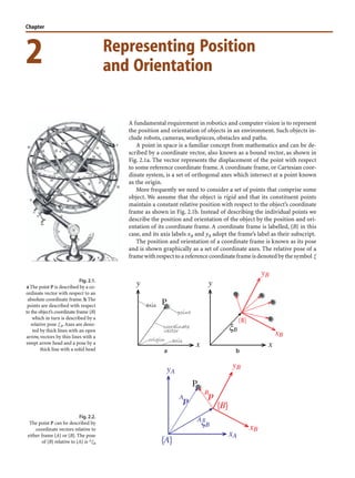
  • 1. 2 Chapter Representing Position and Orientation Fig. 2.1. a The point P is described by a co- ordinate vector with respect to an absolute coordinate frame. b The points are described with respect to the object’s coordinate frame {B} which in turn is described by a relative pose ξB.Axes are deno- ted by thick lines with an open arrow, vectors by thin lines with a swept arrow head and a pose by a thick line with a solid head Fig. 2.2. The point P can be described by coordinate vectors relative to either frame {A} or {B}. The pose of {B} relative to {A} is AξB A fundamental requirement in robotics and computer vision is to represent the position and orientation of objects in an environment. Such objects in- clude robots, cameras, workpieces, obstacles and paths. A point in space is a familiar concept from mathematics and can be de- scribed by a coordinate vector, also known as a bound vector, as shown in Fig. 2.1a. The vector represents the displacement of the point with respect to some reference coordinate frame.A coordinate frame, or Cartesian coor- dinate system, is a set of orthogonal axes which intersect at a point known as the origin. More frequently we need to consider a set of points that comprise some object. We assume that the object is rigid and that its constituent points maintain a constant relative position with respect to the object’s coordinate frame as shown in Fig. 2.1b. Instead of describing the individual points we describe the position and orientation of the object by the position and ori- entation of its coordinate frame. A coordinate frame is labelled, {B} in this case, and its axis labels xB and yB adopt the frame’s label as their subscript. The position and orientation of a coordinate frame is known as its pose and is shown graphically as a set of coordinate axes. The relative pose of a framewithrespecttoareferencecoordinateframeisdenotedbythesymbol ξ
  • 2. 16 – pronounced ksi. Figure 2.2 shows two frames {A} and {B} and the relative pose AξB which describes {B} with respect to {A}. The leading superscript denotes the reference coordinate frame and the subscript denotes the frame being described. We could also think of AξB as describing some motion – imagine picking up {A} and applying a dis- placement and a rotation so that it is transformed to {B}.If the initial superscript is miss- ingweassumethatthechangeinposeisrelativetotheworldcoordinateframedenoted O. The point P in Fig. 2.2 can be described with respect to either coordinate frame. Formally we express this as (2.1) where the right-hand side expresses the motion from {A} to {B} and then to P. The operator · transforms the vector, resulting in a new vector that describes the same point but with respect to a different coordinate frame. An important characteristic of relative poses is that they can be composed or com- pounded. Consider the case shown in Fig. 2.3. If one frame can be described in terms of another by a relative pose then they can be applied sequentially which says,in words,that the pose of {C} relative to {A} can be obtained by compound- ing the relative poses from {A} to {B} and {B} to {C}.We use the operator ⊕ to indicate composition of relative poses. For this case the point P can be described Later in this chapter we will convert these abstract notions of ξ, · and ⊕ into stan- dard mathematical objects and operators that we can implement in MATLAB®. In the examples so far we have shown 2-dimensional coordinate frames. This is appropriate for a large class of robotics problems,particularly for mobile robots which operate in a planar world. For other problems we require 3-dimensional coordinate frames to describe objects in our 3-dimensional world such as the pose of a flying or underwater robot or the end of a tool carried by a robot arm. Fig. 2.3. The point P can be described by coordinate vectors relative to either frame {A}, {B} or {C}. The frames are described by relative poses In relative pose composition we can check that we have our reference frames correct by ensuring that the subscript and superscript on each side of the ⊕ operator are matched.We can then cancel out the intermediate subscripts and superscripts leaving just the end most subscript and superscript which are shown circled. Chapter 2 · Representing Position and Orientation
  • 3. 17 Figure 2.4 shows a more complex 3-dimensional example in a graphical form where we have attached 3D coordinate frames to the various entities and indicated some rela- tive poses. The fixed camera observes the object from its fixed viewpoint and estimates the object’s pose relative to itself.The other camera is not fixed,it is attached to the robot at some constant relative pose and estimates the object’s pose relative to itself. An alternative representation of the spatial relationships is a directed graph (see Appendix J) which is shown in Fig. 2.5. Each node in the graph represents a pose and each edge represents a relative pose.An arrow from X to Y is denoted X ξY and describes the pose of Y relative to X. Recalling that we can compose relative poses using the ⊕ operator we can write some spatial relationships and each equation represents a loop in the graph. Each side of the equation represents a path through the network, a sequence of edges (arrows) that are written in head to tail order. Both sides of the equation start and end at the same node. A very useful property of poses is the ability to perform algebra. The second loop equation says, in words, that the pose of the robot is the same as composing two rela- tive poses: from the world frame to the fixed camera and from the fixed camera to the Fig. 2.4. Multiple 3-dimensional coordi- nate frames and relative poses René Descartes (1596–1650) was a French philosopher,mathematician and part-time mercenary. He is famous for the philosophical statement “Cogito, ergo sum” or “I am thinking, therefore I exist”or“I think, therefore I am”. He was a sickly child and developed a life-long habit of lying in bed and thinking until late morning. A possibly apocryphal story is that during one such morn- ing he was watching a fly walk across the ceiling and realized that he could describe its position in terms of its distance from the two edges of the ceiling. This coordinate system, the Cartesian system, forms the basis of modern (analytic) geometry and influenced the development of mod- ern calculus. In Sweden at the invitation of Queen Christine he was obliged to rise at 5 a.m., breaking his lifetime habit – he caught pneumonia and died. His remains were later moved to Paris, and then moved several times, and there is now some debate about where his remains are. After his death, the Roman Catholic Church placed his works on the Index of Prohibited Books. Chapter 2 · Representing Position and Orientation In mathematical objects terms poses constituteagroup–asetofobjectsthat supports an associative binary operator (composition) whose result belongs to the group, an inverse operation and an identity element.In this case the group is the special Euclidean group in either 2 or 3 dimensions which are commonly referred to as SE(2) or SE(3) respectively.
  • 4. 18 robot. We can subtract ξF from both sides of the equation by adding the inverse of ξF which we denote as ξF and this gives which is the pose of the robot relative to the fixed camera. Fig. 2.5. Spatial example of Fig. 2.4 expressed as a directed graph There are just a few algebraic rules: where 0 represents a zero relative pose. A pose has an inverse which is represented graphically by an arrow from Y to X.Relative poses can also be composed or compounded It is important to note that the algebraic rules for poses are different to nor- mal algebra and that composition is not commutative with the exception being the case where ξ1 ⊕ ξ2 = 0.A relative pose can transform a point expressed as a vector relative to one frame to a vector relative to another So what is ξ? It can be any mathematical object that supports the algebra described above and is suited to the problem at hand. It will depend on whether we are consider- ing a 2- or 3-dimensional problem. Some of the objects that we will discuss in the rest of this chapter include vectors as well as more exotic mathematical objects such as homogeneous transformations, orthonormal rotation matrices and quaternions. For- tunately all these mathematical objects are well suited to the mathematical program- ming environment of MATLAB®. Chapter 2 · Representing Position and Orientation
  • 5. 19 To recap: 1. A point is described by a coordinate vector that represents its displacement from a reference coordinate system; 2. A set of points that represent a rigid object can be described by a single coordinate frame,and its constituent points are described by displacements from that coordinate frame; 3. The position and orientation of an object’s coordinate frame is referred to as its pose; 4. A relative pose describes the pose of one coordinate frame with respect to another and is denoted by an algebraic variable ξ; 5. A coordinate vector describing a point can be represented with respect to a different coordinate frame by applying the relative pose to the vector using the · operator; 6. We can perform algebraic manipulation of expressions written in terms of relative poses. The remainder of this chapter discusses concrete representations of ξ for various common cases that we will encounter in robotics and computer vision. 2.1 lRepresenting Pose in 2-Dimensions A 2-dimensional world, or plane, is familiar to us from high-school Euclidean geom- etry. We use a Cartesian coordinate system or coordinate frame with orthogonal axes denoted x and y and typically drawn with the x-axis horizontal and the y-axis vertical. The point of intersection is called the origin. Unit-vectors parallel to the axes are de- noted ' and (. A point is represented by its x- and y-coordinates (x, y) or as a bound vector (2.2) Figure 2.6 shows a coordinate frame {B} that we wish to describe with respect to the reference frame {A}.We can see clearly that the origin of {B} has been displaced by the vector t = (x, y) and then rotated counter-clockwise by an angle θ. A concrete repre- sentation of pose is therefore the 3-vector AξB ∼ (x, y, θ), and we use the symbol ∼ to denote that the two representations are equivalent. Unfortunately this representation is not convenient for compounding since is a complex trigonometric function of both poses. Instead we will use a different way of representing rotation. The approach is to consider an arbitrary point P with respect to each of the coordi- nate frames and to determine the relationship between Ap and Bp. Referring again to Fig. 2.6 we will consider the problem in two parts: rotation and then translation. Euclid of Alexandria (ca. 325 bce–265 bce) was an Egyptian mathematician who is considered the “father of geometry”. His book Elements deduces the properties of geometrical objects and integers from a small set of axioms. Elements is probably the most successful book in the history of mathematics.It describes plane geometry and is the basis for most people’s first introduction to geometry and formal proof, and is the basis of what we now call Euclidean geometry. Euclidean distance is simply the distance between two points on a plane. Euclid also wrote Optics which describes geometric vision and perspective. 2.1 · Representing Pose in 2-Dimensions
  • 6. 20 To consider just rotation we create a new frame {V} whose axes are parallel to those of {A} but whose origin is the same as {B}, see Fig. 2.7.According to Eq. 2.2 we can express the point P with respect to {V} in terms of the unit-vectors that define the axes of the frame (2.3) which we have written as the product of a row and a column vector. The coordinate frame {B} is completely described by its two orthogonal axes which we represent by two unit vectors which can be written in matrix form as (2.4) Using Eq. 2.2 we can represent the point P with respect to {B} as and substituting Eq. 2.4 we write (2.5) Now by equating the coefficients of the right-hand sides of Eq. 2.3 and Eq. 2.5 we write which describes how points are transformed from frame {B} to frame {V} when the frame is rotated. This type of matrix is known as a rotation matrix and denoted V RB (2.6) Fig. 2.6. Two 2D coordinate frames {A} and {B} and a world point P. {B} is rotated and translated with respect to {A} Chapter 2 · Representing Position and Orientation
  • 7. 21 The rotation matrix VRB has some special properties. Firstly it is orthonormal (also called orthogonal) since each of its columns is a unit vector and the columns are orthogonal. In fact the columns are simply the unit vectors that define {B} with re- spect to {V} and are by definition both unit-length and orthogonal. Secondly,its determinant is +1,which means that R belongs to the special orthogo- nal group of dimension 2 or R ∈ SO(2) ⊂ R2×2. The unit determinant means that the length of a vector is unchanged after transformation, that is, |Bp| = |Vp|, ∀θ. Orthonormal matrices have the very convenient property that R−1 = RT, that is, the inverse is the same as the transpose. We can therefore rearrange Eq. 2.6 as Note that inverting the matrix is the same as swapping the superscript and subscript, which leads to the identity R(−θ) = R(θ )T . It is interesting to observe that instead of representing an angle, which is a scalar, we have used a 2 × 2 matrix that comprises four elements, however these elements are not independent. Each column has a unit magnitude which provides two con- straints. The columns are orthogonal which provides another constraint. Four ele- ments and three constraints are effectively one independent value. The rotation ma- trix is an example of a non-minimum representation and the disadvantages such as the increased memory it requires are outweighed, as we shall see, by its advantages such as composability. The second part of representing pose is to account for the translation between the origins of the frames shown in Fig. 2.6. Since the axes {V} and {A} are parallel this is simply vectorial addition (2.7) (2.8) (2.9) or more compactly as (2.10) Fig. 2.7. Rotated coordinate frames in 2D. The point P can be considered with respect to the red or blue coordinate frame 2.1 · Representing Pose in 2-Dimensions See Appendix D which provides a re- fresher on vectors, matrices and linear algebra.
  • 8. 22 where t = (x, y) is the translation of the frame and the orientation is ARB. Note that ARB = TRB since the axes of {A} and {V} are parallel.The coordinate vectors for point P are now expressed in homogenous form and we write and ATB is referred to as a homogeneous transformation. The matrix has a very specific structure and belongs to the special Euclidean group of dimension 2 or T ∈ SE(2) ⊂ R3×3. By comparison with Eq. 2.1 it is clear that ATB represents relative pose A vector (x, y) is written in homogeneous form as p ∈ P2 , p = (x1, x2, x3) where x = x1/x3,y = x2/x3 and x3 ≠ 0. The dimension has been increased by one and a point on a plane is now represented by a 3-vector. To convert a point to homogeneous form we typically append a one p = (x, y, 1). The tilde indicates the vector is homogeneous. Homogeneous vectors have the important property that p is equivalent to λp, ∀λ ≠ 0 which we write as p λp. That is p represents the same point in the plane irrespective of the overall scaling factor. Homogeneous representation is important for computer vision that we discuss in Part IV. Additional details are provided in Appendix I. A concrete representation of relative pose ξ is ξ ∼ T ∈ SE(2) and T1 ⊕ T2 T1T2 which is standard matrix multiplication. One of the algebraic rules from page 18 is ξ ⊕ 0 = ξ. For matrices we know that TI = T, where I is the identify matrix, so for pose 0 I the identity matrix. Another rule was that ξ ξ = 0. We know for matrices that TT−1 = I which im- plies that T T−1 For a point p ∈ P2 then T·p Tp which is a standard matrix-vector product. To make this more tangible we will show some numerical examples using MATLAB® and the Toolbox. We create a homogeneous transformation using the function se2 >> T1 = se2(1, 2, 30*pi/180) T1 = 0.8660 -0.5000 1.0000 0.5000 0.8660 2.0000 0 0 1.0000 which represents a translation of (1, 2) and a rotation of 30°. We can plot this, relative to the world coordinate frame, by Chapter 2 · Representing Position and Orientation
  • 9. 23 >> axis([0 5 0 5]); >> trplot2(T1, 'frame', '1', 'color', 'b') The options specify that the label for the frame is {1} and it is colored blue and this is shown in Fig. 2.8. We create another relative pose which is a displacement of (2, 1) and zero rotation >> T2 = se2(2, 1, 0) T2 = 1 0 2 0 1 1 0 0 1 which we plot in red >> hold on >> trplot2(T2, 'frame', '2', 'color', 'r'); Now we can compose the two relative poses >> T3 = T1*T2 T3 = 0.8660 -0.5000 2.2321 0.5000 0.8660 3.8660 0 0 1.0000 and plot it, in green, as >> trplot2(T3, 'frame', '3', 'color', 'g'); We see that the displacement of (2, 1) has been applied with respect to frame {1}. It is important to note that our final displacement is not (3, 3) because the displacement is with respect to the rotated coordinate frame. The non-commutativity of composition is clearly demonstrated by >> T4 = T2*T1; >> trplot2(T4, 'frame', '4', 'color', 'c'); and we see that frame {4} is different to frame {3}. Now we define a point (3, 2) relative to the world frame >> P = [3 ; 2 ]; which is a column vector and add it to the plot >> plot_point(P, '*'); Fig. 2.8. Coordinate frames drawn using the Toolbox function trplot2 2.1 · Representing Pose in 2-Dimensions
  • 10. 24 To determine the coordinate of the point with respect to {1} we use Eq. 2.1 and write down and then rearrange as Substituting numerical values >> P1 = inv(T1) * [P; 1] P1 = 1.7321 -1.0000 1.0000 where we first converted the Euclidean point to homogeneous form by appending a one. The result is also in homogeneous form and has a negative y-coordinate in frame {1}. Using the Toolbox we could also have expressed this as >> h2e( inv(T1) * e2h(P) ) ans = 1.7321 -1.0000 where the result is in Euclidean coordinates.The helper function e2h converts Euclid- ean coordinates to homogeneous and h2e performs the inverse conversion.More com- pactly this can be written as >> homtrans( inv(T1), P) ans = 1.7321 -1.0000 The same point with respect to {2} is >> P2 = homtrans( inv(T2), P) P2 = 1 1 2.2 lRepresenting Pose in 3-Dimensions The 3-dimensional case is an extension of the 2-dimensional case discussed in the previous section. We add an extra coordinate axis, typically denoted by z, that is or- thogonal to both the x- and y-axes. The direction of the z-axis obeys the right-hand rule and forms a right-handed coordinate frame. Unit vectors parallel to the axes are denoted ', ( and ) such that (2.11) A point P is represented by its x-, y- and z-coordinates (x, y, z) or as a bound vector Figure 2.9 shows a coordinate frame {B} that we wish to describe with respect to the reference frame {A}.We can see clearly that the origin of {B} has been displaced by the vector t = (x, y, z) and then rotated in some complex fashion. Just as for the 2-dimen- sional case the way we represent orientation is very important. Chapter 2 · Representing Position and Orientation In all these identities, the symbols from left to right (across the equals sign) are a cyclic permutation of the sequence xyz.
  • 11. 25 Our approach is to again consider an arbitrary point P with respect to each of the coordinate frames and to determine the relationship between Ap and Bp. We will again consider the problem in two parts: rotation and then translation. Rotation is surprisingly complex for the 3-dimensional case and we devote all of the next sec- tion to it. 2.2.1 lRepresenting Orientation in 3-Dimensions Any two independent orthonormal coordinate frames can be related by a sequence of rotations (not more than three) about coordinate axes, where no two successive rotations may be about the same axis. Euler’s rotation theorem (Kuipers 1999). Figure 2.9 showed a pair of right-handed coordinate frames with very different orien- tations, and we would like some way to describe the orientation of one with respect to the other. We can imagine picking up frame {A} in our hand and rotating it until it looked just like frame {B}. Euler’s rotation theorem states that any rotation can be con- sidered as a sequence of rotations about different coordinate axes. We start by considering rotation about a single coordinate axis.Figure 2.10 shows a right-handed coordinate frame, and that same frame after it has been rotated by vari- ous angles about different coordinate axes. The issue of rotation has some subtleties which are illustrated in Fig. 2.11. This shows a sequence of two rotations applied in different orders. We see that the final orientation depends on the order in which the rotations are applied.This is a deep and confounding characteristic of the 3-dimensional world which has intrigued mathema- ticians for a long time. The implication for the pose algebra we have used in this chap- ter is that the ⊕ operator is not commutative – the order in which rotations are applied is very important. Mathematicians have developed many ways to represent rotation and we will dis- cuss several of them in the remainder of this section: orthonormal rotation matrices, Euler and Cardan angles, rotation axis and angle, and unit quaternions. All can be represented as vectors or matrices, the natural datatypes of MATLAB® or as a Toolbox defined class. The Toolbox provides many function to convert between these repre- sentations and this is shown diagrammatically in Fig. 2.15. Fig. 2.9. Two 3D coordinate frames {A} and {B}. {B} is rotated and translated with respect to {A} Right-handrule. A right-handed coordinate frame is defined by the first three fingers of your right hand which indicate the relative directions of the x-, y- and z-axes respectively. 2.2 · Representing Pose in 3-Dimensions
  • 12. 26 Rotation about a vector. Wrap your right hand around the vector with your thumb (your x-finger) in the direction of the arrow. The curl of your fingers indicates the direction of increasing angle. Fig. 2.10. Rotation of a 3D coordinate frame. a The original coordinate frame, b–f frame a after various rotations as indicated Fig. 2.11. Example showing the non-com- mutivity of rotation. In the top row the coordinate frame is rota- ted by ü about the x-axis and then ü about the y-axis. In the bottom row the order of rota- tions has been reversed. The results are clearly different Chapter 2 · Representing Position and Orientation
  • 13. 27 2.2.1.1 lOrthonormal Rotation Matrix Just as for the 2-dimensional case we can represent the orientation of a coordinate frame by its unit vectors expressed in terms of the reference coordinate frame. Each unit vector has three elements and they form the columns of a 3 × 3 orthonormal matrix ARB (2.12) which rotates a vector defined with respect to frame {B} to a vector with respect to {A}. Thematrix Rbelongstothespecialorthogonalgroupof dimension 3orR ∈ SO(3) ⊂ R3×3. It has the properties of an orthonormal matrix that were mentioned on page 16 such as RT = R−1 and det(R) = 1. The orthonormal rotation matrices for rotation of θ about the x-, y- and z-axes are The Toolbox provides functions to compute these elementary rotation matrices,for example Rx(θ ) is >> R = rotx(pi/2) R = 1.0000 0 0 0 0.0000 -1.0000 0 1.0000 0.0000 Such a rotation is also shown graphically in Fig. 2.10b. The functions roty and rotz compute Ry(θ ) and Rz(θ ) respectively. The corresponding coordinate frame can be displayed graphically >> trplot(R) which is shown in Fig. 2.12a. We can visualize a rotation more powerfully using the Toolbox function tranimate which animates a rotation >> tranimate(R) showing the world frame rotating into the specified coordinate frame. 2.2 · Representing Pose in 3-Dimensions Reading the columns of an orthonormal rotation matrix from left to right tells us the directions of the new frame’s axes in terms of the current coordinate frame. For example if R = 1.0000 0 0 0 0.0000 -1.0000 0 1.0000 0.0000 the new frame has its x-axis in the old x-direction (1, 0, 0),its y-axis in the old z-direction (0, 0, 1), and the new z-axis in the old negative y-direction (0, −1, 0).In this case the x-axis was unchanged since this is the axis around which the rotation occurred.
  • 14. 28 To illustrate compounding of rotations we will rotate the frame of Fig. 2.12a again, this time around its y-axis >> rotx(pi/2) * roty(pi/2) ans = 0.0000 0 1.0000 1.0000 0.0000 -0.0000 -0.0000 1.0000 0.0000 >> trplot(R) to give the frame shown in Fig. 2.12b. In this frame the x-axis now points in the direc- tion of the world y-axis. The non-commutativity of rotation can be shown by reversing the order of the rotations above >> roty(pi/2)*rotx(pi/2) ans = 0.0000 1.0000 0.0000 0 0.0000 -1.0000 -1.0000 0.0000 0.0000 which has a very different value. We recall that Euler’s rotation theorem states that any rotation can be represented by not more than three rotations about coordinate axes. This means that in general an arbitrary rotation between frames can be decomposed into a sequence of three rota- tion angles and associated rotation axes – this is discussed in the next section. The orthonormal matrix has nine elements but they are not independent. The col- umns have unit magnitude which provides three constraints.The columns are orthogo- nal to each other which provides another three constraints. Nine elements and six constraints is effectively three independent values. 2.2.1.2 lThree-Angle Representations Euler’s rotation theorem requires successive rotation about three axes such that no two successive rotations are about the same axis. There are two classes of rotation sequence: Eulerian and Cardanian, named after Euler and Cardano respectively. The Eulerian type involves repetition, but not successive, of rotations about one particular axis: XYX, XZX, YXY, YZY, ZXZ, or ZYZ. The Cardanian type is character- ized by rotations about all three axes: XYZ, XZY, YZX,YXZ, ZXY, or ZYX. In common usage all these sequences are called Euler angles and there are a total of twelve to choose from. Fig. 2.12. Coordinate frames displayed using trplot. a Reference frame rotated by ü about the x-axis, b frame a rotated by ü about the y-axis Chapter 2 · Representing Position and Orientation If the column vectors are ci , i ∈ 1 3 then c1 · c2 = c2 · c3 = c3 · c1 = 0.
  • 15. 29 It is common practice to refer to all 3-angle representations as Euler angles but this is underspecified since there are twelve different types to choose from.The par- ticularanglesequenceisoftenaconventionwithinaparticulartechnologicalfield. The ZYZ sequence (2.13) is commonly used in aeronautics and mechanical dynamics,and is used in the Toolbox. The Euler angles are the 3-vector ¡ = (φ, θ, ψ). For example, to compute the equivalent rotation matrix for ¡ = (0.1, 0.2, 0.3) we write >> R = rotz(0.1) * roty(0.2) * rotz(0.3); or more conveniently >> R = eul2r(0.1, 0.2, 0.3) R = 0.9021 -0.3836 0.1977 0.3875 0.9216 0.0198 -0.1898 0.0587 0.9801 The inverse problem is finding the Euler angles that correspond to a given rotation matrix >> gamma = tr2eul(R) gamma = 0.1000 0.2000 0.3000 However if θ is negative >> R = eul2r(0.1 , -0.2, 0.3) R = 0.9021 -0.3836 -0.1977 0.3875 0.9216 -0.0198 0.1898 -0.0587 0.9801 the inverse function >> tr2eul(R) ans = -3.0416 0.2000 -2.8416 returns a positive value for θ and quite different values for φ and ψ. However the cor- responding rotation matrix >> eul2r(ans) ans = 0.9021 -0.3836 -0.1977 0.3875 0.9216 -0.0198 0.1898 -0.0587 0.9801 is the same – the two different sets of Euler angles correspond to the one rotation matrix. The mapping from rotation matrix to Euler angles is not unique and always returns a positive angle for θ. Leonhard Euler (1707–1783) was a Swiss mathematician and physicist who dominated eighteenth century mathematics. He was a student of Johann Bernoulli and applied new mathematical tech- niques such as calculus to many problems in mechanics and optics. He also developed the func- tional notation, y = F(x), that we use today. In robotics we use his rotation theorem and his equa- tions of motion in rotational dynamics. He was prolific and his collected works fill 75 volumes. Almost half of this was produced dur- ing the last seventeen years of his life when he was completely blind. 2.2 · Representing Pose in 3-Dimensions
  • 16. 30 For the case where θ = 0 >> R = eul2r(0.1 , 0, 0.3) R = 0.9211 -0.3894 0 0.3894 0.9211 0 0 0 1.0000 the inverse function returns >> tr2eul(R) ans = 0 0 0.4000 which is quite different. For this case the rotation matrix from Eq. 2.13 is since Ry = I and is a function only of the sum φ + ψ. For the inverse operation we can therefore only determine this sum, and by convention φ = 0. The case θ = 0 is a singu- larity and will be discussed in more detail in the next section. Another widely used convention is the roll-pitch-yaw angle sequence angle (2.14) which are intuitive when describing the attitude of vehicles such as ships, aircraft and cars. Roll, pitch and yaw (also called bank, attitude and heading) refer to rotations aboutthe x-,y-,z-axes,respectively.ThisXYZanglesequence,technicallyCardanangles, are also known as Tait-Bryan angles or nautical angles. For aerospace and ground vehicles the x-axis is commonly defined in the forward direction, z-axis downward and the y-axis to the right-hand side. For example >> R = rpy2r(0.1, 0.2, 0.3) R = 0.9752 -0.0370 0.2184 0.0978 0.9564 -0.2751 -0.1987 0.2896 0.9363 and the inverse is >> gamma = tr2rpy(R) gamma = 0.1000 0.2000 0.3000 The roll-pitch-yaw sequence allows all angles to have arbitrary sign and it has a singu- larity when θp = ±ü which is fortunately outside the range of feasible attitudes for most vehicles. Chapter 2 · Representing Position and Orientation Named after Peter Tait a Scottish physi- cistandquaternionsupporter,andGeorge Bryan an early Welsh aerodynamicist. Notethatmostroboticstexts(Paul1981; Siciliano et al. 2008; Spong et al. 2006) swap the x- and z-axes by defining the heading direction as the z- rather than x-direction,that is roll is about the z-axis not the x-axis. This was the con- vention in the Robotics Toolbox prior to Release 8. The default in the Toolbox is now XYZ order but the ZYX order can be specified with the‘zyx’option. Gerolamo Cardano (1501–1576) was an Italian Renaissance mathematician, physician, astrolo- ger, and gambler. He was born in Pavia, Italy, the illegitimate child of a mathematically gifted lawyer. He studied medicine at the University of Padua and later was the first to describe ty- phoid fever.He partly supported himself through gambling and his book about games of chance Liber de ludo aleae contains the first systematic treatment of probability as well as effective cheating methods. His family life was problematic: his eldest son was executed for poisoning his wife, and his daughter was a prostitute who died from syphilis about which he wrote a treatise. He computed and published the horoscope of Jesus, was accused of heresy, and spent time in prison until he abjured and gave up his professorship. He died on the day he had pre- dicted astrologically. He published the solutions to the cubic and quartic equations in his book Ars magna in 1545, and also invented the combination lock, the gimbal consisting of three concentric rings allowing a compass or gyroscope to rotate freely (see Fig. 2.13), and the Cardan shaft with universal joints which is used in vehicles today.
  • 17. 31 2.2.1.3 lSingularities and Gimbal Lock A fundamental problem with the three-angle representations just described is singu- larity. This occurs when the rotational axis of the middle term in the sequence be- comes parallel to the rotation axis of the first or third term. This is the same problem as gimbal lock, a term made famous in the movie Apollo 13. A mechanical gyroscope used for navigation such as shown in Fig. 2.13 has as its innermost assembly three orthogonal gyroscopes which hold the stable member stationary with respect to the universe. It is mechanically connected to the spacecraft via a gimbal mechanism which allows the spacecraft to move around the stable platform without exerting any torque on it. The attitude of the spacecraft is deter- mined by measuring the angles of the gimbal axes with respect to the stable platform – giving a direct indication of roll-pitch-yaw angles which in this design are a Cardanian YZX sequence. Consider the situation when the rotation angle of the middle gimbal (rotation about the spacecraft’s z-axis) is 90° – the axes of the inner and outer gimbals are aligned and they share the same rotation axis. Instead of the original three rotational axes, since two are parallel, there are now only two effective rotational axes – we say that one degree of freedom has been lost. In mathematical, rather than mechanical, terms this problem can be seen using the definition of the Lunar module’s coordinate system where the rotation of the spacecraft’s body-fixed frame {B} with respect to the stable platform frame {S} is For the case when θr = ü we can apply the identity leading to which cannot represent rotation about the y-axis. This is not a good thing because spacecraft rotation about the y-axis will rotate the stable element and thus ruin its precise alignment with the stars. The loss of a degree of freedom means that mathematically we cannot invert the transformation,we can only establish a linear relationship between two of the angles. In such a case the best we can do is determine the sum of the pitch and yaw angles. We observed a similar phenomena with the Euler angle singularity earlier. 2.2 · Representing Pose in 3-Dimensions “TheLMBodycoordinatesystemisright- handed, with the +X axis pointing up through the thrust axis, the +Y axis pointing right when facing forward whichisalongthe+Zaxis.Therotational transformation matrix is constructed by a 2-3-1 Euler sequence, that is: Pitch about Y, then Roll about Z and, finally, Yaw about X.Positive rotations are pitch up,roll right, yaw left.”(Hoag 1963). Operationallythiswasasignificantlim- iting factor with this particular gyro- scope(Hoag1963)andcouldhavebeen alleviatedbyaddingafourthgimbal,as was used on other spacecraft. It was omitted on the Lunar Module for rea- sons of weight and space. Rotations obey the cyclic rotation rules Rx(ü) Ry(θ ) Rx(ü)T ≡ Rz(θ ) Ry(ü) Rz(θ ) Ry(ü)T ≡ Rx(θ ) Rz(ü) Rx(θ ) Rz(ü)T ≡ Ry(θ ) and anti-cyclic rotation rules Ry(ü)T Rx(θ ) Ry(ü) ≡ Rz(θ ) Rz(ü)T Ry(θ ) Rz(ü) ≡ Rx(θ ). Mission clock: 02 08 12 47 Flight:“Go,Guidance.” Guido: “He’s getting close to gimbal lock there.” Flight: “Roger. CapCom, recommend he bring up C3, C4, B3, B4, C1 and C2 thrusters, and ad- vise he’s getting close to gimbal lock.” CapCom: “Roger.” Apollo 13, mission control communications loop (1970) (Lovell and Kluger 1994, p 131; NASA 1970).
  • 18. 32 All three-angle representations of attitude, whether Eulerian or Cardanian, suffer this problem of gimbal lock when two consecutive axes become aligned. For ZYZ- Euler angles this occurs when θ = kπ, k ∈ Z and for roll-pitch-yaw angles when pitch θp = ±(2k + 1)ü. The best that can be hoped for is that the singularity occurs for an attitude which does not occur during normal operation of the vehicle – it requires judicious choice of angle sequence and coordinate system. Singularities are an unfortunate consequence of using a minimal representation. To eliminate this problem we need to adopt different representations of orientation. Many in the Apollo LM team would have preferred a four gimbal system and the clue to success, as we shall see shortly in Sect. 2.2.1.6, is to introduce a fourth parameter. 2.2.1.4 lTwo Vector Representation For arm-type robots it is useful to consider a coordinate frame {E} attached to the end-effector as shown in Fig. 2.14. By convention the axis of the tool is associated with the z-axis and is called the approach vector and denoted $ = (ax, ay, az).For some applications it is more convenient to specify the approach vector than to specify Euler or roll-pitch-yaw angles. However specifying the direction of the z-axis is insufficient to describe the coordi- nate frame – we also need to specify the direction of the x- and y-axes.An orthogonal vector that provides orientation, perhaps between the two fingers of the robot’s grip- per is called the orientation vector,& = (ox, oy, oz).These two unit vectors are sufficient to completely define the rotation matrix Fig. 2.13. Schematic of Apollo Lunar Module (LM) inertial measure- ment unit (IMU). The vehicle’s coordinate system has the y-axis pointing up through the thrust axis, the z-axis forward, and the y-axis pointing right. Starting at the stable platform {S} and working outwards toward the spacecraft’s body frame {B} the rotation angle sequence is YZX. The components labelled Xg, Yg and Zg are the x-, y- and z-axis gyroscopes and those labelled Xa, Ya and Za are the x-, y- and z-axis accelerometers (Apollo Opera- tions Handbook, LMA790-3-LM) Chapter 2 · Representing Position and Orientation
  • 19. 33 (2.15) since the remaining column can be computed using Eq. 2.11 as % = & × $. Even if the two vectors $ and & are not orthogonal they still define a plane and the computed % is normal to that plane. In this case we need to compute a new value for &′ = $× % which lies in the plane but is orthogonal to each of $ and %. Using the Toolbox this is implemented by >> a = [1 0 0]'; >> o = [0 1 0]'; >> oa2r(o, a) ans = 0 0 1 0 1 0 -1 0 0 Any two non-parallel vectors are sufficient to define a coordinate frame. For a camera we might use the optical axis,by convention the z-axis,and the left side of the camera which is by convention the x-axis. For a mobile robot we might use the gravitational acceleration vector (measured with accelerometers) which is by convention the z-axis and the heading direction (measured with an electronic compass) which is by convention the x-axis. 2.2.1.5 lRotation about an Arbitrary Vector Two coordinate frames of arbitrary orientation are related by a single rotation about some axis in space. For the example rotation used earlier >> R = rpy2r(0.1 , 0.2, 0.3); we can determine such an angle and vector by >> [theta, v] = tr2angvec(R) theta = 0.3816 v = 0.3379 0.4807 0.8092 where theta is the amount of rotation and v is the vector around which the rotation occurs. Fig. 2.14. Robot end-effector coordinate system defines the pose in terms of an approach vector $ and an orientation vector &, from which % can be computed (courtesy of lynxmotion.com) 2.2 · Representing Pose in 3-Dimensions So long as they are not parallel.
  • 20. 34 This information is encoded in the eigenvalues and eigenvectors of R. Using the builtin MATLAB® function eig >> [v,lambda] = eig(R) v = 0.6655 0.6655 0.3379 -0.1220 - 0.6079i -0.1220 + 0.6079i 0.4807 -0.2054 + 0.3612i -0.2054 - 0.3612i 0.8092 lambda = 0.9281 + 0.3724i 0 0 0 0.9281 - 0.3724i 0 0 0 1.0000 the eigenvalues are returned on the diagonal of the matrix lambda and the corre- sponding eigenvectors are the corresponding columns of v. An orthonormal rotation matrix will always have one real eigenvalue at λ = 1 and a complex pair λ = cosθ ± i sinθ where θ is the rotation angle. From the definition of eigenvalues and eigenvectors we recall that where v is the eigenvector corresponding to λ. For the case λ = 1 then which implies that the corresponding eigenvector v is unchanged by the rotation. There is only one such vector and that is the one about which the rotation occurs. In the example the third eigenvalue is equal to one, so the rotation axis is the third col- umn of v. Converting from angle and vector to a rotation matrix is achieved using Rodrigues’ rotation formula Our familiar example of a rotation of ü about the x-axis can be found by >> R = angvec2r(pi/2, [1 0 0]) R = 1.0000 0 0 0 0.0000 -1.0000 0 1.0000 0.0000 It is interesting to note that this representation of an arbitrary rotation is parameter- ized by four numbers: three for the rotation axis, and one for the angle of rotation. However the direction can be represented by a unit vector with only two parameters since the third element can be computed by giving a total of three parameters. Alternatively we can multiply the unit vector by the angle to give another 3-parameter representation vθ.While these forms are minimal Olinde Rodrigues (1795–1850) was a French-Jewish banker and mathematician who wrote ex- tensively on politics, social reform and banking. He received his doctorate in mathematics in 1816 from the University of Paris, for work on his first well known formula which is related to Legendre polynomials. His eponymous rotation formula was published in 1840 and is perhaps the first time the representation of a rotation as a scalar and a vector was articulated.His formula is sometimes,and inappropriately,referred to as the Euler-Rodrigues formula.He is buried in the Pere-Lachaise cemetery in Paris. Chapter 2 · Representing Position and Orientation S(·) is the skew-symmetric matrix de- fined in Eq.3.5 and also Appendix D.
  • 21. 35 and efficient in terms of data storage they are analytically problematic. Many variants have been proposed including v sin(θ/2) and v tan(θ) but all are ill-defined for θ = 0. 2.2.1.6 lUnit Quaternions Quaternions came from Hamilton after his really good work had been done; and, though beautifully ingenious, have been an unmixed evil to those who have touched them in any way, including Clark Maxwell. Lord Kelvin, 1892 Quaternions have been controversial since they were discovered by W. R. Hamilton over 150 years ago but they have great utility for roboticists. The quaternion is an ex- tension of the complex number – a hyper-complex number – and is written as a scalar plus a vector (2.16) where s ∈ R,v ∈ R3 and the orthogonal complex numbers i,j and k are defined such that (2.17) We will denote a quaternion as One early objection to quaternions was that multiplication was not commutative but as we have seen above this is exactly the case for rotations. Despite the initial contro- versy quaternions are elegant, powerful and computationally straightforward and widely used for robotics, computer vision, computer graphics and aerospace inertial navigation applications. In the Toolbox quaternions are implemented by the Quaternion class. The con- structor converts the passed argument to a quaternion, for example >> q = Quaternion( rpy2tr(0.1, 0.2, 0.3) ) q = 0.98186 < 0.064071, 0.091158, 0.15344 > 2.2 · Representing Pose in 3-Dimensions The multiplication rules are the same as for cross products of the orthogonal vectors ', ( and ). Sir William Rowan Hamilton (1805–1865) was an Irish mathematician, physicist, and astrono- mer. He was a child prodigy with a gift for languages and by age thirteen knew classical and modern European languages as well as Persian,Arabic,Hindustani,Sanskrit,and Malay.Hamilton taught himself mathematics at age 17, and discovered an error in Laplace’s Celestial Mechanics. He spent his life at Trinity College, Dublin, and was appointed Professor of Astronomy and Royal Astronomer of Ireland while still an undergraduate. In addition to quaternions he contributed to the development of optics, dynamics, and algebra. He also wrote poetry and corresponded with Wordsworth who advised him to devote his energy to mathematics. According to legend the key quaternion equation, Eq. 2.17, occured to Hamilton in 1843 while walking along the Royal Canal in Dublin with his wife, and this is commemorated by a plaque on Broome bridge: Here as he walked by on the 16th of October 1843 Sir William Rowan Hamilton in a flash of genius discovered the fundamental formula for quaternion multiplication i2 = j2 = k2 = i j k = −1 & cut it on a stone of this bridge. His original carving is no longer visible,but the bridge is a pilgrimage site for mathematicians and physicists.
  • 22. 36 To represent rotations we use unit-quaternions.These are quaternions of unit mag- nitude, that is, those for which |h| = 1 or s2 + v1 2 + v2 2 + v3 2 = 1. For our example >> q.norm ans = 1.0000 The unit-quaternion has the special property that it can be considered as a rotation of θ about the unit vector % which are related to the quaternion components by (2.18) and is similar to the angle-axis representation of Sect. 2.2.1.5. For the case of quaternions our generalized pose is ξ is ξ ∼ h ∈ Q and which is known as the quaternion or Hamilton product, and which is the quaternion conjugate. The zero pose 0 1 <0, 0, 0> which is the identity quaternion. A vector v ∈ R3 is rotated h · v hh(v)h−1 where h(v) = 0, <v> is known as a pure quaternion. Chapter 2 · Representing Position and Orientation If we write the quaternion as a 4-vector (s,v1,v2,v2) then multiplication can be expressed as a matrix-vector product where Compounding two orthonormal rota- tion matrices requires 27 multiplica- tions and 18 additions.The quaternion form requires 16 multiplications and 12 additions.Thissavingcanbeparticu- larly important for embedded systems. The Quaternion class overloads a number of standard methods and functions. Quaternion multiplication is invoked through the overloaded multiplication operator >> q = q * q; and inversion, the quaternion conjugate, is >> q.inv() ans = 0.98186 < -0.064071, -0.091158, -0.15344 > Multiplying a quaternion by its inverse >> q*q.inv() ans = 1 < 0, 0, 0 > or >> q/q ans = 1 < 0, 0, 0 > results in the identity quaternion which represents a null rotation. The quaternion can be converted to an orthonormal rotation matrix by >> q.R ans = 0.9363 -0.2896 0.1987 0.3130 0.9447 -0.0978 -0.1593 0.1538 0.9752 and we can also plot the orientation represented by a quaternion >> q.plot() which produces a result similar in style to that shown in Fig. 2.12.
  • 23. 37 A 3-vector passed to the constructor yields a pure quaternion >> Quaternion([1 2 3]) ans = 0 < 1, 2, 3 > which has a zero scalar component.A vector is rotated by a quaternion using the over- loaded multiplication operator >> q*[1 0 0]' ans = 0.9363 0.3130 -0.1593 The Toolbox implementation is quite complete and the Quaternion has many meth- ods and properties which are described fully in the online documentation. 2.2.2 lCombining Translation and Orientation We return now to representing relative pose in three dimensions, the position and orientation change, between two coordinate frames as shown in Fig. 2.9. We have discussed several different representations of orientation, and we need to combine this with translation, to create a tangible representation of relative pose. The two most practical representations are: the quaternion vector pair and the 4 × 4 homoge- neous transformation matrix. For the vector-quaternion case ξ ∼ (t, h) where t ∈ R3 is the Cartesian position of the frame’s origin with respect to the reference coordinate frame,and h ∈ Q is the frame’s orientation with respect to the reference frame. Composition is defined by and negation is and a point coordinate vector is transformed to a coordinate frame by Alternatively we can use a homogeneous transformation matrix to describe rota- tion and translation. The derivation is similar to the 2D case of Eq. 2.10 but extended to account for the z-dimension The Cartesian translation vector between the origin of the coordinates frames is t and the change in orientation is represented by a 3 × 3 orthonormal submatrix R. The vectors are expressed in homogenous form and we write 2.2 · Representing Pose in 3-Dimensions
  • 24. 38 (2.19) and ATB is a 4 × 4 homogeneous transformation.The matrix has a very specific struc- ture and belongs to the special Euclidean group of dimension 3 or T ∈ SE(3) ⊂ R4×4. A concrete representation of relative pose ξ is ξ ∼ T ∈ SE(3) and T1 ⊕ T2 T1T2 which is standard matrix multiplication. (2.20) One of the rules of pose algebra from page 18 is ξ ⊕0 = ξ. For matrices we know that TI = T, where I is the identify matrix, so for pose 0 I the identity matrix. Another rule of pose algebra was that ξ ξ = 0. We know for matrices that TT−1 = I which implies that T T−1 (2.21) The 4 × 4 homogeneous transformation is very commonly used in robotics and computer vision,is supported by the Toolbox and will be used throughout this book as a concrete representation of 3-dimensional pose. The Toolbox has many functions to create homogeneous transformations. For ex- ample we can demonstrate composition of transforms by >> T = transl(1, 0, 0) * trotx(pi/2) * transl(0, 1, 0) T = 1.0000 0 0 1.0000 0 0.0000 -1.0000 0.0000 0 1.0000 0.0000 1.0000 0 0 0 1.0000 The function transl create a relative pose with a finite translation but no rotation, and trotx returns a 4 × 4 homogeneous transform matrix corresponding to a rota- tion of ü about the x-axis: the rotation part is the same as rotx(pi/2) and the translational component is zero. We can think of this expression as representing a walk along the x-axis for 1 unit,then a rotation by 90° about the x-axis and then a walk of 1 unit along the new y-axis which was the previous z-axis. The result, as shown in the last column of the resulting matrix is a translation of 1 unit along the original x-axis and 1 unit along the original z-axis. The orientation of the final pose shows the effect of the rotation about the x-axis. We can plot the corresponding coordinate frame by >> trplot(T) The rotation matrix component of T is >> t2r(T) ans = 1.0000 0 0 0 0.0000 -1.0000 0 1.0000 0.0000 and the translation component is a vector >> transl(T)' ans = 1.0000 0.0000 1.0000 Chapter 2 · Representing Position and Orientation Many Toolbox functions have variants that return orthonormal rotation ma- trices or homogeneous transforma- tions,forexample,rotxandtrotx, rpy2r and rpy2tr etc. Some Toolbox functions accept an ortho- normal rotation matrix or a homoge- neous transformation and ignore the translational component, for example, tr2rpy or Quaternion.
  • 25. 39 2.3 lWrapping Up In this chapter we learned how to represent points and poses in 2- and 3-dimensional worlds. Points are represented by coordinate vectors relative to a coordinate frame. A set of points that belong to a rigid object can be described by a coordinate frame, and itsconstituentpointsaredescribedbydisplacementsfromtheobject’scoordinateframe. The position and orientation of any coordinate frame can be described relative to another coordinate frame by its relative pose ξ. Relative poses can be applied sequen- tially (composed or compounded), and we have shown how relative poses can be ma- nipulated algebraically. An important algebraic rule is that composition is non-com- mutative – the order in which relative poses are applied is important. 2.3 · Wrapping Up Table 2.1. Summary of the various concrete representations of pose ξ introduced in this chapter Fig. 2.15. Conversion between rotational representations
  • 26. 40 We have explored orthonormal rotation matrices for the 2- and 3-dimensional case to represent orientation and its extension, the homogeneous transformation matrix, to represent orientation and translation. Rotation in 3-dimensions has subtlety and complexity and we have looked at other representations such as Euler angles, roll- pitch-yaw angles and quaternions. Some of these mathematical objects are supported natively by MATLAB® while others are supported by functions or classes within the Toolbox. There are two important lessons from this chapter. The first is that there are many mathematical objects that can be used to represent pose and these are summarized in Table 2.1. There is no right or wrong – each has strengths and weaknesses and we typically choose the representation to suit the problem at hand. Sometimes we wish for a vectorial representation in which case (x, y, θ) or (x, y, z, ¡ ) might be appropri- ate,but this representation cannot be easily compounded.Sometime we may only need to describe 3D rotation in which case Γ or h is appropriate.The Toolbox supports con- versions between many different representations as shown in Fig. 2.15. In general though, we will use homogeneous transformations throughout the rest of this book. The second lesson is that coordinate frames are your friend. The essential first step in many vision and robotics problems is to assign coordinate frames to all objects of interest, indicate the relative poses as a directed graph, and write down equations for the loops.Figure 2.16 shows you how to build a coordinate frame out of paper that you can pick up and rotate. We now have solid foundations for moving forward. The notation has been defined and illustrated, and we have started our hands-on work with MATLAB®. The next chapter discusses coordinate frames that change with time,and after that we are ready to move on and discuss robots. Further Reading The treatment in this chapter is a hybrid mathematical and graphical approach that covers the 2D and 3D cases by means of abstract representations and operators which are later made tangible. The standard robotics textbooks such as Spong et al. (2006), Craig (2004), Siciliano et al. (2008) and Paul (1981) all introduce homogeneous trans- formation matrices for the 3-dimensional case but differ in their approach.These books also provide good discussion of the other representations such as angle-vector and 3-angle representations. Spong et al. (2006, Sec 2.5.1) have a good discussion of singularities.Siegwart et al.(2011) explicitly cover the 2D case in the context of mobile robot navigation. Hamilton and his supporters, including Peter Tait, were vigourous in defending Hamilton’s precedence in inventing quaternions, and for muddying the water with respect to vectors which were then beginning to be understood and used. Rodrigues developed the key idea in 1840 and Gauss discovered it in 1819 but, as usual, did not Chapter 2 · Representing Position and Orientation Fig. 2.16. Build your own coordinate frame. a Get the PDF file from http:// www.petercorke.com/axes.pdf; bcut it out, fold along the dotted lines and add a staple.Voila!
  • 27. 41 publish it. Quaternions had a tempestuous beginning. The paper by Altmann (1989) is an interesting description on this tussle of ideas, and quaternions have even been wo- ven into fiction (Pynchon 2006). Quaternions are discussed briefly in Siciliano et al. (2008). The book by Kuipers (1999) is a very readable and comprehensive introduction to quaternions. Quaternion interpolation is widely used in computer graphics and animation and the classic pa- per by Shoemake (1985) is very readable introduction to this topic. The first publica- tions about quaternions for robotics is probably Taylor (1979) and with subsequent work by Funda (1990). Exercises 1. Explore the effect of negative roll, pitch or yaw angles. Does transforming from RPY angles to a rotation matrix then back to RPY angles give a different result to the starting value as it does for Euler angles? 2. Explore the many options associated with trplot. 3. Use tranimate to show translation and rotational motion about various axes. 4. Animate a tumbling cube a) Write a function to plot the edges of a cube centred at the origin. b) Modify the function to accept an argument which is a homogeneous transfor- mation which is applied to the cube vertices before plotting. c) Animate rotation about the x-axis. d) Animate rotation about all axes. 5. Using Eq. 2.21 show that TT−1 = I. 6. Generate the sequence of plots shown in Fig. 2.11. 7. Where is Descarte’s skull? 8. Create a vector-quaternion class that supports composition, negation and point transformation. 2.3 · Wrapping Up