This document discusses the key elements of highway geometric design including cross-section elements, sight distance considerations, horizontal and vertical alignment details, and intersection elements. It covers factors that affect highway geometric design such as design speed, topography, traffic, capacity, and environmental factors. It provides details on cross-section components, sight distance requirements, horizontal and vertical curves, and overtaking sight distance calculations. The objective of highway geometric design is to provide efficient traffic operation with maximum safety at reasonable cost.

1. 1
1

2. Importance of geometric design
•The geometric design of a highway deals with the
dimensions and layout of visible features of the highway
such as alignment, sight distance and intersection.
The main objective of highway design is to provide optimum
efficiency in traffic operation with maximum safety at reasonable
cost.
•
• Geometric design of highways
elements :
 Cross section elements
 Sight distance considerations
 Horizontal alignment details
 Vertical alignment details
 Intersection elements
deals with following
2

3. FACTORS AFFECTING HIGHWAY
GEOMETRICS DESIGN
•
•
•
•
•
Design speed
Topography
Traffic factors
Design hourly volume and capacity
Environmental and other factors
Design speed
•In India different speed standards have
for different class of road.
been assigned
• The maximum safe speed of vehicles used for
the road geometrics design is known as design
speed. 3

4. Design speed is important for the following…
 Sight distance
 Super Elevation
 Radius of horizontal curve
 Extra widening of pavement
 Length of valley curves
4

5. topography
• Classified based on the general
 Plane terrain- <10%
 Rolling terrain- 10-25%
 Mountainous terrain- 25-60%
 Steep terrain- >60%
slope of the country.
Traffic factor
• Vehicular characteristics and human
road users.
characteristics of
• Different vehicle classes have different speed and
acceleration characteristics, different dimensions and
weight .
Human factor includes the physical, mental and
psychological characteristics of driver and pedestrian.
•
5

6. Topography(Cont.)
8/16/2016 Highway Geometric Design 25
6

7. Topography(Cont.)
8/16/2016 Highway Geometric Design 26
7

8. Topography(Cont.)
8/16/2016 Highway Geometric Design 27
8

9. Steep terrain slope >60%
9

10. Design hourly volume and capacity
•
•
Traffic flow fluctuating with time
Low value during off-peak hours to the highest
value during the peak hour.
• It is uneconomical to
traffic flow.
design the roadwayforpeak
Environmental factors
Aesthetics
Landscaping
Air pollution
Noise pollution
10

11. Cross Section Of Road And Its
Componentss
•
•
•
•
•
•
•
•
•
•
Carriageway
Shoulder
Side slope
Berm
Boundary stone
Side drain
Roadway or formation width
Right of way
Building line
Control line
11

12. Cross-section of Road
12

13. 1. Carriage way:-
The width of pavement way on which vehicles travel is called Carriage
way or pavement width.
Width of carriageway is determined on the basis of the width of the
vehicle and the minimum side clearance for safety.
As per IRC specification, the maximum width of vehicle is 2.44m.
Formation width is the top of width of the highway embankment
excluding the side drains.
Formation width = width of carriage way + width of shoulders
2. Formation width:-
13

14. Carriage way
Formation width
14

15. Two lane two-way road
carriageway
15

16. WIDTH OF ROADWAY OF VARIOUS CLASSES OF ROADS
SL. No. Road classification Roadway wisth
Plane and rolling terrain Mountainous and steep
terrain
1 NH & SH
a) Single lane 12
b) two lane 12
6.25
8.80
2 MDR
a) Single lane 9
b) two lane 9
4.75
4.75
3 ODR
a) Single lane 7.5
b) two lane 9
4.75
4.75
4 Village roads-single lane 7.5 4
WIDTH OF CARRIAGEWAY
SL. NO. Class of road Width of carriageway in ‘m’
1 Single lane 3.75
2 Two lane without raised kerbs 7.0
3 Two lane with raised kerbs 7.5
4 Intermediate lane 5.5
5 Multilane pavement 3.5/lane
16

17.  Shoulders are provided along the road edge to serve as an
emergency lane for vehicles .
 As per IRC, the min. width of shoulder should be 2.5m.
 Uses :
 Repair of broken down vehicles
 Overtaking operations
 To act as an emergency lane
 For future widening of road
 For temp. diversion of traffic during road repair etc
It should have sufficient load bearing capacity even in wet weather.
The surface of the should be rougher than the traffic lanes so that
vehicles are discouraged to use the shoulder as a regular traffic.
The colour should be different from that of the pavement so
as to be distinct.
Shoulders
17

18. shoulders
18

19. Treated
shoulderunTreated
shoulder
19

20. 20

21. 21

22. 5. Side slope:-
The slope of earthwork in filling or in cutting is called Side
slope. It imparts stability to the earthwork.
• For Filling:
Normally, 1:2
• For cutting:
Type of soil Slope
1:1 to
1:1/2
Ordinary soil
Broken Rock
Soft Rock
1:1/2 to 1:1/4
1:1/4 to 1:1/8
Hard Rock Approx. Perpendicular
22

23. 23

24. 6. Berm:-
The distance between the road toe and the inner edge of
borrow pit is called berm.
It prevents the erosion of embankment soil.
7. Boundary stone :-
To indicate the boundary of land acquired for road, stones
are driven in to the ground at about 30m distance on either
side from the center line of the road. These stones are
known as boundary stone.
24

25. 25

26. 8. Side drain:-
For the drainage of rainwater, drains are provided on either
side of the road. Normally, side drains are required for the
road in cutting. For road in embankment, side drain is not
necessary.
9. Building line:-
The distance from the center line of road on either side,
within which construction of buildings is not permitted is
called Building line.
26

27. 27

28. 10.Control line:-
At the locations like bank, hospital, factory, theatre,
etc. on the road, where more people gather
disturbance to the traffic will be more.
Purposes :
For future widening of road
To reduce the chance of accidents
To relieve residents from noise pollution
To prevent disturbance to the traffic by nearby residents
 The distance from the centre line to such building is called control
line.
28

29. Type of road B.L(m) C.L(m)
NH, SH 40 75
MDR 30 55
ODR 20 35
VR 12 24
29

30. Cross section of different types of road as per IRC :
30

31. 31

32. Cross slope or camber:
• It is the slope provided to the road surface in the
transverse direction to drain off the rain water
from the road surface.
To prevent the entry of surface water into the
subgrade soil through pavement.
To prevent the entry of water into the bituminous
pavement layer.
To remove the rain water from the pavement
surface as quick as possible and to allow the
pavement to get dry soon after the rain.
It is expressed as a percentage or 1V:Nh.
It depends on the pavement surface and amount
of rainfall.
•
•
•
•
•
32

33. Shape of the cross slope:
•
•
•
Parabolic shape(fast moving vehicle)
Straight line
Combination of parabolic and straight line
Recommended values of camber for different types of road surface
Sl no. Type of road surface Range of camber in areas of rain
fall range
heavy light
1 Cement concrete and high type 1 in 50(2%)
bituminous pavement
1 in 60(1.7%)
2 Thin bituminous surface 1 in 40(2.5%) 1 in 50(2%)
3 Water bound macadam(WBM) and gravel I in 33(3%)
pavement
1 in 40(2.5%)
4 Earth 1 in 25(4%) 1 in 33(3%) 33

34. 34

35. SIGHT DISTANCE
35
Definition :
 The actual distance along the road surface , which a driver
from a specified height above the carriageway has visibility of
stationary or moving object is known as sight distance.
2

36.  Restrictions to sight distance may be caused as shown in fig.
• Sight distance at horizontal curve
http://www.tpub.com/inteng/11.htm16.gif 3
36

37. • Sight distance at vertical curve
http://www.msha.gov/training/surfhaul/images/slide6.jpg
3
7
37

38. • Sight distance at intersection
3
8
http://onlinemanuals.txdot.gov/txdotmanuals/rdw/images/3-2.png 38

39. 39

40. 4
0
40

41. Stoppingsightdistance
(SSD)
41
Definition : The minimum sight distance available on a highway
to stop a vehicle travelling at design speed , safely without
collision with any other obstruction is called stopping distance.
https://encrypted-tbn1.gstatic.com/images?q=tbn:ANd9GcQFKpIxAAAbJH3n64ECpY2EHIf-
mjYUXedmQ0WUPheL5hqfngHS 7

42. 42

43. http://www.ite.org/css/online/img/Figure10-5.jpg 43
•For the purpose of measuring stopping sight distance , IRC
has suggest clear sight triangle as shown in fig. ,

44. Factorsaffectingstoppingsightdistance
44

45. 1) speed of vehicle:
45
https://encrypted/tbn1.gstatic.com/images?q=tbn:ANd9GcTJk56HWGT5GXbpWSsGFElb5384HgIeyKfqcB4cqKwu9xy69dSm

46. 2) total reaction time of the driver :
46
http://www.hk/phy.org/contextual/mechanics/kin/eq_motion/6-01.gif

47. 3) friction resistance between the road &tyres :
47https://www.koroad.or.kr/images/en/img_know38.jpg

48. 4) gradient of road:
48

49. http://webarchive.nationalarchives.gov.uk/20061101091400/http://ordnancesurv
ey.co.uk/images/userImages/misc/education/gradient.gif 49

50. Analysisof
SSD:
50

51. Lagdistance
• reaction time is known as lag distance .
• Reaction time of the driver is the time
taken from the instant the object is visible to
the driver to the instant the brakes are
effectively applied.
51
Definition : The distance travelled by the vehicle during the total
16http://www.hk/phy.org/contextual/mechanics/kin/eq_motion/6-01.gif

52. WhatisPIEVTheory?
52
Acc. To PIEV theory the total reaction time of the driver is split
into four parts .
52

53. 1) Perception time :
It is the time required for the sensations received by the
eyes or ears to be transmitted to the brain through the
nervous system .
2) Intellection time :
 It is the time required for understanding the situation.
53
53

54. http://www.arrivealive.co.za/images/stoppingdistance.jpg
https://m2.behance.net/rendition/pm/703187/disp/859cc9a079eca4b5556af04b
3aa6215c.png
54
54

55. 3) Emotion time :
 it is time elapsed during emotional sensations & Disturbance
such as fear , anger ,etc. with reference to the situation .
4) Volition time :
 volition time is the time taken for the final action.
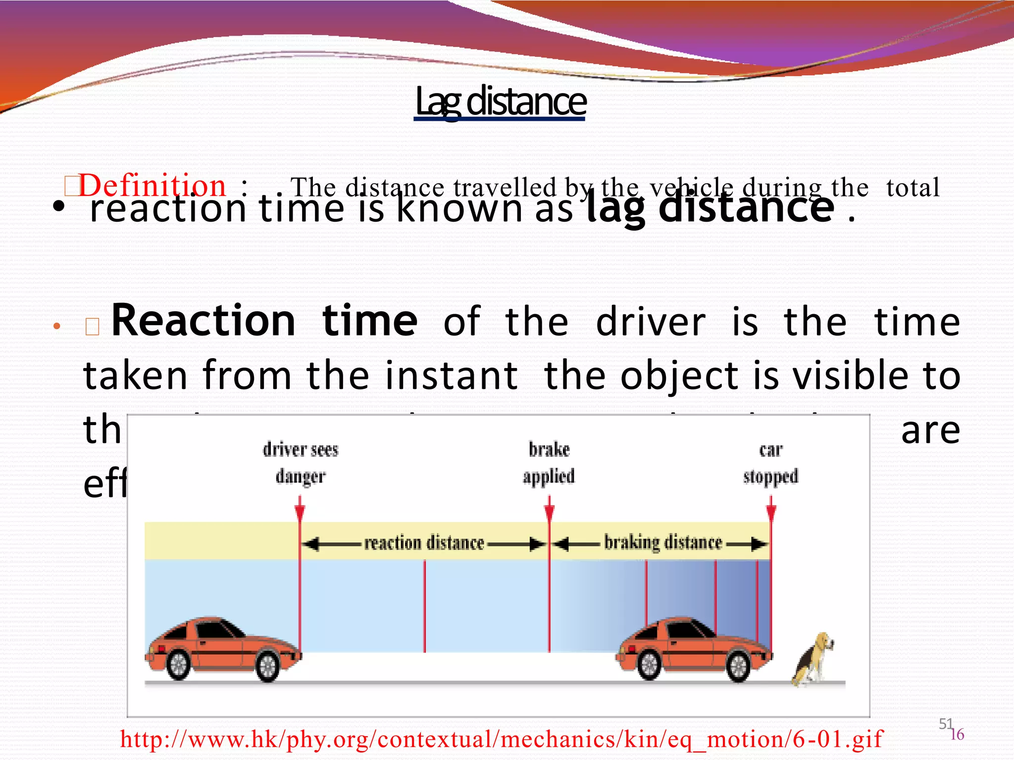
Lag distance = v * t
55
Where, v = speed of vehicle in m/s
t = total reaction time (s) [ as per IRC t = 2.5 s ]
g= acceleration due to gravity = 9.8 m/sec2
f= coefficient of friction (0.4 to 0.35) 55

56. Braking distance= v²/2gf
SSD=lag distance + braking distance
•
•
Two-way traffic single lane road: SSD=2*SSD
In one-way traffic with single or more lane or two-
way traffic with more than single lane: Minimum
SSD= SSD
Table 2.6: Coefficient of longitudinal friction
Speed, kmph 30 40 50 60 ˃80
Longitudinal
coefficient of
friction
0.40 0.38 0.37 0.36 0.35
SSD= V.t + v²/2gf
56

57. Example-1
• Calculate the safe stopping sight distance for design
speed of 50kmph for(a) two-way traffic on two lane
road (b)two-way traffic on single lane road
Example-2
• Calculate the minimum sight distance required to avoid
a head on collision of two cars approaching from
opposite direction at 90 and 60kmph.coefficient
friction of 0.7 and a brake efficiency of 50%, in either
case
Example-3
• Calculate the stopping sight distance on a highway at
descending gradient of 2% for design speed of 80
kmph, assume other data as per IRC specification.
a

58. OVERTAKING SIGHT DISTANCE
 The minimum distanceopen to thevision of thedriver
of a vehicle intending to overtake slow vehicle ahead
with safety against the traffic of opposite direction is
known as the minimum overtaking sight
distance(OSD)orthe safe passing sightdistance.
The overtaking sight distance or OSD is the distance
measured along the centre of the road which a driver
with his eye level 1.2m above the road surfacecan see the
topof an object 1.2m above the road surface

59. 59
Factors on which overtaking sight distance
depends:
•Minimum OSD required for the safe overtaking
depends on:
a. Speed of overtaking, overtaken vehicle and vehicle
coming from opposite direction if any.
b. Skill and reaction time of the driver.
c. Distance between overtaking and overtaken vehicles.
d. Rate of acceleration of overtaking vehicle
e. Gradient of the road if any.

60. Analysis of OSD on a two lane road with
two way traffic:
60

61. wheret is the reaction time of thedriver in second= 2 sec.

62. 62
•From A1 to A2, the distance ‘d1’ (m) travelledby
overtaking vehicle Aat reduced speed ‘vb’ (m/s)
during reaction time ‘t’(sec),
d1= vb X t
• IRC suggest reaction time t of driver as 2 sec ,
d1= 2vb
•From A2 to A3, vehicle Astarts accelerating, shift
to adjoining lane, overtakes vehicle B, and shift
back to its original lane during overtaking time ‘T’
(sec) and travel distance ‘d2’(m).

63. 63
•From A2 to A3, the distance ‘d2’ (m) is further
split into three parts viz;
d2= (s+b+s)
d2= (b+2s)
•The minimum spacing ‘s’ (m)between vehicles
depends on their speed and is given by empirical
formula,
s=(0.7vb + 6)
•The distance covered by the slow vehicle B
travelling at a speed of ‘vb’ (m/s) in time ‘T’(sec) is,
b= vb X T

64. • The overtaking time ‘T’ (sec) is calculatedas;
d2=(b+2s)=(vbT+aT2/2)
b=vb T , 2s=aT2/2
•From C1 to C2, distance travelled by vehicle C
moving at design speed ‘v’ (m/s) during time ‘T’
(sec) is given by,
d3=v X T
64

65. 65
• Thus overtaking sight distance (OSD) is,
OSD=(d1+d2+d3)
OSD= (vb X t) + (vb X T +2s) +(v X T)
• If speed is in kmph,
OSD= (0.28Vb X t)+(0.28Vb X T+2s)+(0.28V X T)
•In case speed of overtaken vehicle is not given it
is assumed 16 kmph less than design speed of the
highway.

66. where,
s=spacing of vehicles
t=reaction time of driver = 2sec
v =design speed in m/sec
V= design speed in kmph
vb=initial speed of overtaking vehicle in m/sec
Vb=initial speed of overtaking vehicle in
Kmph
A=average acceleration in kmph/sec
a=average acceleration in m/sec2
66

67. 67
Super elevation (e):
•In order to counteract the effect of centrifugal
force and to reduce the tendency of the vehicle to
overturn or skid, the outer edge of the pavement is
raised with respect to the inner edge, thus providing
a transverse slope throughout the length of the
horizontal curve.
•This transverse inclination to the pavement
surface is known as Super elevation or cant or
banking.

68. 68

70. • Therefore, the general equation for the design of
super elevation is given by,
e + f = v²∕gR
70
• If ‘V’ speed of the vehicle is in kmph,
e + f = V²∕ 127R
where,
e=rate of Superelevation=tanӨ
f = design value of lateral friction
coefficient = 0.15
v = speed of the vehicle, m/sec
R = radius of the horizontal curve, m
g = acceleration due to gravity = 9.81 m/sec²

71. 71
Maximum Superelevation
•Indian Roads Congress (IRC) had fixed the
maximum limit of Superelevation in plan and
rolling terrains and is snow bound areas as 7.0 %.
•On hill roads not bound by snow a maximum
Superelevation upto10% is recommended.
•On urban road stretches with frequent
intersections, it may be necessary to limit the
maximum Superelevation to 4.0 %.

72. 72
Widening of pavement on horizontal curves:
On horizontal curves, especially when they are
Less than 300m radii, it is common to widen the pavement
slightly more than the normal width.
• Widening is needed for the following reasons:
a. An automobile has a rigid wheel base and only the front
wheels can be turned, when this vehicle takes a turn to
negotiate a horizontal curve, the rear wheel do not follow
the same path as that of the front wheels. This phenomenon
is called off tracking.

73. 73
b.While two vehicle cross or overtake at horizontal curve
there is psychological tendency to maintain a greater
clearance between the vehicle for safety.
c.For greater visibility at curve, the driver have tendency
not to follow the central path of the lane, but to use the
outer side at the beginning of the curve.
d.At higher speed superelevation and lateral friction
cannot counteract centrifugal force and skidding may
occur.

74. 74
Analysis of extra widening on horizontal curves:
The extra widening of pavement on
horizontal curves is divided into two parts:
a. Mechanical widening/Off tracking
b. Psychological widening

75. a. Mechanical widening/Off tracking (Wm):
75

76. 76
•If road having ‘n’ traffic lanes and ‘n’ vehiclescan
travel simultaneously, mechanical widening reqd. is
given by,
Wm = nl2/ 2R
Where,
R = Mean radius of the curve in m,
n=no. of traffic lanes
l = Length of Wheel base of longest vehicle , m
(l = 6.0 m or 6.1m for commercial vehicles)
V= design speed, kmph

77. b. Psychological widening (Wps):
An empirical formula has been recommended
by IRC for deciding the additional psychological
widening.
•The psychological widening is given by the
formula:
77

78. • The total extra widening is given by,
We=Wm + Wps
where,
n=no. of traffic lanes
l = length of wheel base =6.1 or 6 m
V=design speed kmph
R = radius of the horizontal curve, m
78

79. Horizontal transition curves
 When a non circular curve is introduce between a
straight and a circular curve has a varying radius which
decreases from infinity at the straight end (tangent
point) to the desired radius of the circular curve at the
other end (curve point) for the gradual introduction of
centrifugal force is known as transition curve.

80. Objectives for providing transition curve
 To introduce gradually the centrifugal force between
the tangent point and the beginning of the circular
curve, avoiding sudden jerk on the vehicle. This
increases the comfort of passengers.
 To enable the driver turn the steering gradually for his
own comfort and security
 To provide gradual introduction of super elevation
 To provide gradual introduction of extra widening.
 To enhance the aesthetic appearance of the road.

82. Type of transition curve
 spiral or clothoid
 cubic parabola
 Lemniscate

83. Length of transition curve
 Case-1:Rate of change of centrifugal
acceleration
 Where,
 Ls= length of transition curve in ‘m’
 C= allowable rate of change of centrifugal
accleration,
 R= Radius of the circular curve in ‘m’

84.  case-2:Rate of introduction of super-elevation
 If the pavement is rotated about the center line.
If the pavement is rotated about the inner edge
 Where ,
 W is the width of pavement
 We is the extra widening
 Rate of change of superelevation of 1 in N

85.  case-3:By empirical formula
 According to IRC standards:
 For plane and rolling terrain:
 For mountainous and steep
 terrain:
 NOTE: The design length of transition curve(Ls) will
be the highest value of case-1,2 and 3

86. 86
Gradients:
•Gradient is the rate of rise or fall along the
length of road with respect to the horizontal.
•It is expressed as a ratio of 1 in n or also as
percentage such as n%.
‘

87. 87
The following are the various factors which
govern the selection of gradient in the
alignment of a road.
1. Nature of ground
2. Nature of traffic
3. Drainage required.
4. The type of road surface.
5. The total height to be curved.

88. 1. Ruling Gradient: The gradient usually adopted while
making the alignment of a road is called as ruling
Gradient.
2. Limiting Gradient:
The gradient steeper then the ruling which may be
used in restricted road lengths where the later is not
feasible is called maximum or Limiting Gradient.
3. Exceptional Gradient:
The gradient steeper than the limiting which may be
used in short lengths of the road only in extra ordinary
situtation is called as Exceptional Gradient.

90. 4. Average Gradient: The total rise or fall between any
two points along the alignment of a road divided by the
horizontal distance between them is called Average
Gradient.
5. Floating Gradient:
The gradient on which a motor vehicle moving with a
constant speed, continues to descend with the same
speed without any application of power or brakes is
called Floating Gradient.
6. Minimum Gradient:
The minimum desirable slope essential for effective
drainage of rain water from the road surface is called
Minimum Gradient.

92. Grade compensation
 At the horizontal curve, due to the turning angle α of the
vehicle, the curve resistance develop is equal to T(1-
Cosα).
 Thus grade compensation can be defined as the reduction
in gradient at the horizontal curve because of the
additional tractive force required due to curve resistance
(T−Tcosα), which is intended to offset the extra tractive
force involved at the curve.

93. 93
 IRC gave the following specification for the grade
compensation.
1.Grade compensation is not required for grades
flatter than 4% because the loss of tractive force
is negligible.
2.Grade compensation is (30+R)/R %, where ‘R’
is the radius of the horizontal curve in meters.
3.The maximum grade compensation is limited to
75/R%.

95. 95
Vertical Curves:
•The vertical curves used in highway may be
classified into two categories:
a. Summit curves or crest curves
b. Valley curves or sag curves
‘

96. a. Summit curves or crest curves:
‘
96

97. 97
Length of summit curve:
•While designing the length the parabolic summit
curves, it is necessary to consider SSD and OSD
Separately.
‘

98. 98
•Length of summit curve for stopping sight
distance (SSD):
Two cases are considered in deciding the length:
a. When L>SSD
b. When L<SSD
‘

99. a. When L > SSD
The general equation for length of curve
is given by:
• Substituting the value of H=1.2m and h=0.15m,
‘
99

100. b. When L < SSD
The general equation for length of curve is
given by:
• Substituting the value of H=1.2m and h=0.15m,
•The minimum radius of the parabolic summit
curve is calculated from relation R=L/N
‘
100

101. 101
•Length of summit curve for overtaking sight
distance (OSD):
Two cases are considered in deciding the length:
a. When L > OSD
b. When L < OSD
‘

102. a. When L > OSD
The general equation for length of curve
is given by:
• Substituting the value of H=1.2m,
‘
120

103. b. When L < OSD
The general equation for length of curve
is given by:
• Substituting the value of H=1.2m,
‘
103

104. 104
wher
e,
• N= deviation angle i.e. algebraic
difference between two grade
• H=height of driver eye above carriageway i.e.
• 1.2 m
• h=height of object above carriageway i.e. 0.15
m L=length of summit curve, m
• S=sight distance i.e. SSD or OSD

105. 105
Length of valley curve:
•The important factors to be considered in valley
curve design are:
a.Impact free movement of vehicles at design
speed or comfort to passenger.
b.Providing adequate sight distance under head
lights of vehicles for night driving
c.Locating lowest point of valley curve for
providing suitable cross drainage facilities
‘

106. b. Valley curves or sag curves:
‘
106

107. a. Length of valley transition curve for comfort
condition:
Total length of valley curve is given by:
If ‘V’ is inkmph,
‘
107

108. 108
where,
v or V= design speed in m/sec or kmph
C=allowable rate of change of centrifugal
acceleration=0.6 m/sec3
L=length of valley curve=2Ls
N= deviation angle i.e. algebraic difference
between two grade

109. 109
b. Length of valley curve for head light sight
distance:
•The length of valley curve for head light sight
distance may be determined for two condition:
a. When L > SSD
b. When L < SSD
‘

110. a. When L > SSD
The general equation for length of valley
curve is given by:‘
110

111. b. When L < SSD
The general equation for length of valley
curve is given by:
where,
N= deviation angle i.e. algebraic difference
between two grade
L=total length of valley curve, m
S=SSD, m
‘
111