The document outlines the geometric design of highways, focusing on dimensions, alignments, sight distances, and safety standards required for efficient traffic operation. Key factors influencing the design include design speed, terrain, traffic characteristics, and environmental considerations, with detailed elements such as cross sections, camber, and superelevation discussed. Various road features such as carriageways, shoulders, sidewalks, and medians are described along with their functions in enhancing road safety and traffic management.

1. 12/27/2024
1
GEOMETRIC DESIGN OF
HIGHWAYS
Geometric design:
 Geometric design of a highways deals with the dimensions and layout of visible features of the
highway such as horizontal and vertical alignments, sight distances and intersections and fixation of
standards with respect to various components.
 The geometrics of highway should be designed to provide efficiency in traffic operations with
maximum safety at reasonable cost.
 It is important to plan and design the geometric features of the road during the initial alignment itself
taking into consideration the future growth of traffic flow and possibility of the road being upgraded to
a higher category or to a higher design speed standard at a later stage.
 Geometric design of highways deals with following elements:
(i) Cross section elements
(ii) Sight distance considerations
(iii) Horizontal alignment details
(iv) Vertical alignment details
(v) Intersection elements

2. 12/27/2024
2
3.1 Factors controlling geometric design of highway
The geometric design of highways depends on several design factors. The
important factors which control the geometric elements are:
(a) Design speed
(b) Topography or terrain
(c) Traffic factors
(d) Design hourly volume and capacity
(e) Environmental and other factors
Design speed:
• Design speed is the maximum permissible continuous speed of vehicles
which it can travel with safety on highway when weather conditions and
other factors are as per standard.
• The design speed is the most important factor controlling the geometric
design elements of highways. Design of almost every geometric design
element of a road is dependent on the design speed.
• For example, the requirements of the pavement surface characteristics, the
cross section element of the road such as, width and clearance requirements,
the sight distance requirements are decided based on the design speed of the
road.
• Also the horizontal alignment elements such
as radius of curve, super elevation, transition
curve length and the vertical alignment
Elements such as gradient, length of summit
and valley curves depend mainly on the design
speed of the road.
Topography or terrain
• According to NRS 2070, Terrain is classified according to the percent slope
of the country across road alignment (Table below). Percent slope can be
estimated by counting the number of 1 m contours crossed by a 100 m long
line. While classifying the terrain, short stretches of varying terrain should
be ignored.
Table 3.2: Terrains classification based on the general slope of the country
Degree
Percent cross slope
Terrain type
S.N
0-5.7
0-10
Plain
1
> 5.7-14
> 10-25
Rolling
2
> 14-31
> 25-60
Mountainous
3
> 31
>60
Steep
4

3. 12/27/2024
3
Traffic Factors
• The traffic factors such as vehicular characteristics and human characteristics also control design of
highway geometrics.
• Static and dynamic characteristics of vehicles (here static characteristics are: dimension and weight of
vehicles, dynamic characteristics are: acceleration, break efficiency) and the physical, mental,
psychological characteristics of the drivers and Pedestrians also effects the design of highway.
Design hourly volume and capacity
• The traffic flow or volume keeps fluctuating with time, from a low value during The certain off-peak
hours to the higher flow during the peak hours.
• It will be uneconomical to design the roadway facilities for the peak traffic flow or the highest hourly
traffic volume.
• Therefore a reasonable value of traffic volume is decided for the design and this is called the 'design
hourly volume’.
• Traffic capacity is the ability of a roadway to accommodate traffic. It is
expressed as the maximum number of vehicle in a road that can pass a given
point in an hour, i.e., 'vehicles per hour per lane.
• The maximum theoretical capacity is calculated by
C = 1000 V/ S
Here, C = Capacity of single lane, vehicle per hour
V = Speed of vehicle
S = c/c spacing between the vehicles or sight distance
Environmental and other factors
• The environmental factors such as aesthetics, landscaping, air pollution,
noise pollution and other local conditions should be given due consideration
in the design of road geometrics.
• Some of the arterial high speed highways and expressways are designed for
higher speed standards and uninterrupted flow of vehicles by providing
controlled access and grade separated intersections.

4. 12/27/2024
4
3.2 Cross-Sectional Elements
• The characteristics of cross-sectional elements are important in highway geometric design because they
influence the safety and comfort.
• The cross sectional elements of a highway pavement are
a) Width of Carriage way
b) Shoulder
c) Camber
d) Median
e) Kerb
f) Road Margin
g) Width of Formation
h) Right of Way (RoW)
Width of Carriage Way (C/W) or Width of Pavement
• It may be defined as that strip of road which is constructed for the movement
of vehicular traffic.
• The carriageway generally consists of hard surface to facilitate smooth
movement and is made of either hard bituminous treated materials or cement
concrete.
• It is also called Pavement width.
Shoulders
• Serves for an emergency stop of vehicles.
• Used to laterally support the pavement structure.
• In practice in Nepal according to NRRS 2071; width of shoulder = 0.5 to 1.5
m. According to NRS 2070
IV
III
II
I
1.5m
2 m
2.5 m
3.75 m

5. 12/27/2024
5
Advantages of shoulder
• Provides space for parking vehicles during repair etc.
• Capacity of road increased because of frequently available opportunity for
overtaking.
• Sufficient space available for parking vehicles on rest.
• Provides space for fixing traffic signs away from the pavement.
• Shady trees can be grown up away from the pavement.
• Provides sufficient space for confidence in driving.
• Proper drainage strengthen the life of the pavement.
• Increased effective width of carriageway.
• Lateral clearance increases the sight distance.
Roadway
• It is the portion of road which is covered by carriageway and shoulders on
both side and the central reservation (median, strip etc) if any.
• It is the top width of road measure perpendicular to the axis of road at the
finished road level.
• Roadway = Carriage way +2 × Shoulder
Right of Way (Row) or Land Width
The strip of land on either side of road from its center line () acquired during
road development and which is under the control of road authority (DoR Nepal)
i) National Highway = 25 m on either side
ii) Feeder Roads = 15 m on either side
iii) District Roads = 10 m on either side
iv) City Roads = as NH for 4-lane and as per FR for 2-lane
Right of way may be used for the following purposes
• To accumulate drainage facilities.
• To provide frontage roads/driveways in roads with controlled access.
• To develop road side arboriculture.
• To open side burrow pits.
• To improve visibility in curves.
• To accommodate various road ancillaries.
• To widen the road where required in future with no compensation for
property.

6. 12/27/2024
6
Building Line: It represents a line on either side of the road between which no
building activity is permitted at all to reserve sufficient space for future
improvement of roads.
Control line: It represents the nearest limits of future uncontrolled building
activity in relation to road to exercise control of the nature of building up to set
back distance up to the control lines.
Sidewalk or Foot Path
• It is that portion of urban road which is provided for the movement of
pedestrian traffic where the intensity is high.
• Minimum width 1.5 m.
• According to NRS 2070
Width in m
Flow of pedestrian number
1.5 m
Up to 500
2 m
500-1500
2.5 m
1500-2500
3 m
greater 2500
Kerb
• It is that element of road which separates vehicular traffic from pedestrians
by providing physical barrier (15-20 cm).
Median Strip (or Traffic Separator or Central Reservations)
• It is the raised portion of the central road strip within the roadway
constructed to separate traffic following in one direction from the traffic in
opposite direction.
Road margins
• The portion of the road beyond the edge of the roadway up to the road
boundary is generally called road margin.
• It includes the frontage road, driveway, footpath, embankment slope, etc.

7. 12/27/2024
7
3.2.1 Elements of Cross-Sections for Urban Roads
Along with the above mentioned cross sectioned elements, some additional
cross section elements are considered for the urban road, they are:
1. Parking Lanes
• Parking lanes are provided in urban lanes for side parking. Parallel parking
is preferred because it is safe for the vehicles moving on the road. The
parking lane should have a minimum of 3.0 m width in the case of parallel
parking.
2. Bus-bays
• Bus bays are provided by recessing the kerbs for bus stops. They are
provided so that they do not obstruct the movement of vehicles in the
carriage way. They should be at least 75 meters away from the intersection
so that the traffic near the intersections is not affected by the bus-bays.
3. Service Roads
• Service roads, or frontage roads, run parallel to a main road and allow local
traffic to gain access to property.. They are usually isolated by a separator
and access to the highway will be provided only at selected points.
• These roads are provided to avoid congestion in the expressways and also
the speed of the traffic in those lanes is not reduced.
4. Cycle Track
• Cycle tracks are provided in urban areas when the volume of cycle traffic is
high. Minimum width of 2 meter is required, which may be increased by 1
meter for every additional track.
5. Footpath
• Footpaths are exclusive right of way to pedestrians, especially in urban
areas. They are provided for the safety of the pedestrians when both the
pedestrian traffic and vehicular traffic is high.
• Minimum width is 1.5 meter and may be increased based on the traffic. The
footpath should be either as smooth as the pavement or more smoother than
that to induce the pedestrian to use the footpath.

8. 12/27/2024
8
6. Guard Rails
• They are provided at the edge of the shoulder usually when the road is on an
embankment. They serve to prevent the vehicles from running off the
embankment, especially when the height of the fill exceeds 3 m.
• Guard stones painted in alternate black and white are usually used. They also
give better visibility of curves at night under headlights of vehicles.
7. Median Strip
• The median strip is the reserved area that separates opposing lanes of traffic
on divided roadways, such as divided highways, dual carriageways, freeway
and motorways.
• The term also applies to divided roadways other than highways, such as
some major streets in urban or suburban areas. Median strip are provided
with following objectives.
i. To segregate traffic coming from opposite direction.
ii. To segregate slow and fast moving traffic in same direction.
iii. To channelize traffic into streams at intersection.
iv. To prevent head on collision between vehicle moving from opposite
direction.
v. To provide aesthetic beauty,
Kerb
• Kerb indicates the boundary between carriageway and shoulder in rural
roads and the boundary between carriageway and footpaths or parking
spaces in urban roads. The height of kerbs ranges from 10 to 20 cm.
• Kerbs can be designed on the basis of their functions as given below;
i. Low kerb/mountable type kerb
ii. Semi-barrier type
iii. Barrier type
iv. Submerged kerb

9. 12/27/2024
9
Functions:
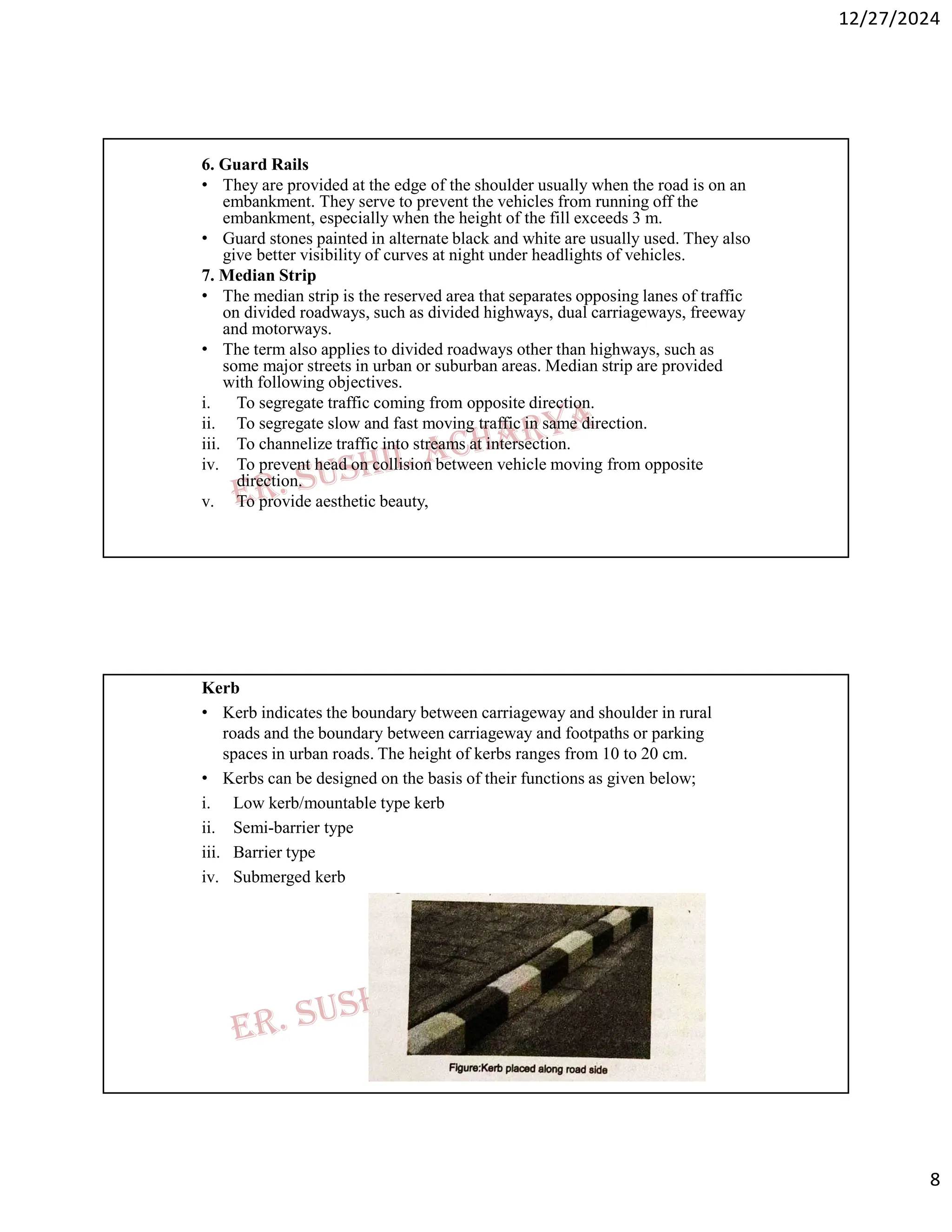
• To separate different lanes of road.
• To strengthen and protect pavement edge. To facilitate and control drainage
• To provide good aesthetic appearance.
3.2.1 Rural Roads
District road/ core network(in hill)
3.2.2Camber or Cross Slope or Cross Fall
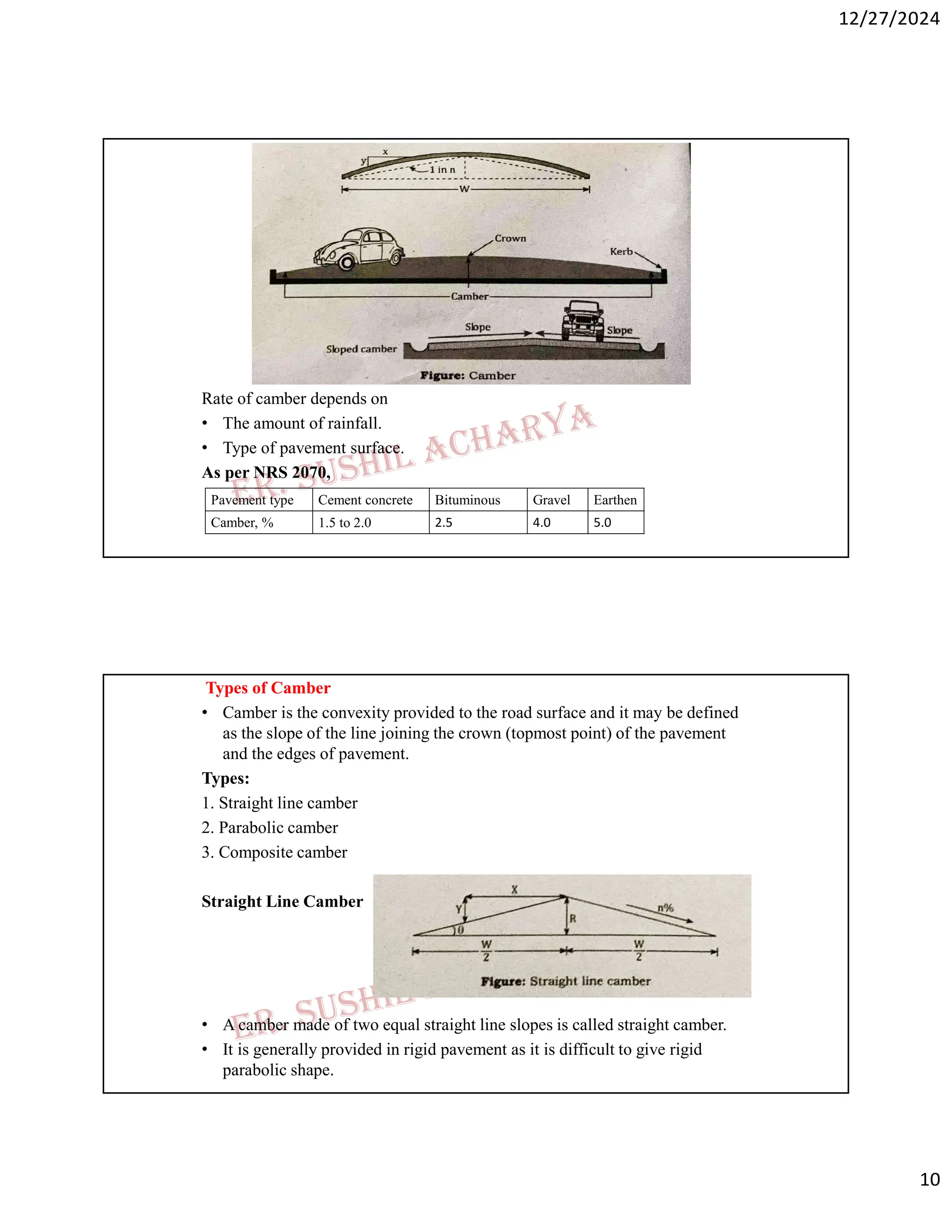
• A Camber is the cross slope provided to raise middle of the road surface in
the transverse direction to drain off rain water from road surface. It is
expressed as % or 1 in N
Objectives of Camber
The main objectives of providing camber for road construction are:
• Surface protection[Mainly for the bituminous or gravel roads].
• Facilitate quick drying of the Pavement. This helps to increase the safety.
• Proper drainage which helps to protect the sub-grade.

10. 12/27/2024
10
Rate of camber depends on
• The amount of rainfall.
• Type of pavement surface.
As per NRS 2070,
Earthen
Gravel
Bituminous
Cement concrete
Pavement type
5.0
4.0
2.5
1.5 to 2.0
Camber, %
Types of Camber
• Camber is the convexity provided to the road surface and it may be defined
as the slope of the line joining the crown (topmost point) of the pavement
and the edges of pavement.
Types:
1. Straight line camber
2. Parabolic camber
3. Composite camber
Straight Line Camber
• A camber made of two equal straight line slopes is called straight camber.
• It is generally provided in rigid pavement as it is difficult to give rigid
parabolic shape.

11. 12/27/2024
11
• The wheel tyres are not fully in contact with road surface and high stress
may develop.
In figure
w = width of road
n = camber provided/cross slope
R= difference in level between crown and edge
From figure
tanθ = y/x
Also, tanθ = ⁄
=
If tanθ = n
or, y = n*x
or, n =
or, y =
𝟐𝑹
𝒘
* x
which is required equation.
Parabolic Camber
• A camber with a shape of simple quadratic parabola is termed as parabolic
camber.
• It is generally provided in flexible pavement (bituminous).
• The road surface is flatter at the middle and steeper near the edge.
• It provides favorable condition for overtaking at higher speed.
In parabola, y varies as x² i.e., y = a x²
or, x² = ( ⁄ )²
n = tanθ
𝑜𝑟,
x²
= ²
n = ⁄
or, x² = ²
n =
or,
x²
= . 𝑛
or, y = 𝑥²
Parabolic camber is provided where fast moving vehicles are run.

12. 12/27/2024
12
Composite Camber
• The camber in road which consists
of two straight slopes from edges with
a circular or parabolic crown in the
center of carriage way is called as
composite camber.
Necessity/Advantages of Camber
• To drain of surface water quickly.
• To prevent infiltration into
underlying pavement layers and
sub- grade.
• To give the driver a physiological
feelings of the presence of two lanes.
• To improve the road appearance.
3.2.3 Superelevation
In order to counteract the effect of centrifugal force and to reduce the tendency
of the vehicle to overturn or skid, the outer edge of the pavement is raised with
respect to the inner edge, thus providing a transverse slope throughout the
length of the horizontal curve. This transverse inclination to the pavement
surface is known as "superelevation' or cant or banking.
 The rate of superelevation, 'e' is expressed as the ratio of the height of outer
edge with respect to the horizontal width.
Fig. Superelevated pavement section
 From Fig. it may be seen that the
outer edge of the pavement is
raised by NL = E
Here,
For small value of θ, sin θ ≈ tan θ
so, tan θ= = e
∴e =
sin θ = =
E
B
E
B
E
B
NL
MN

13. 12/27/2024
13
Purpose of Providing Superelevation in Roads
a. To counteract the effect of centrifugal force acting on the moving vehicle.
b. To prevent the damaging effect on the surface of the roads due to improper
distribution of load on the roads.
c. To reduce the number of accidents.
d. To help the fast-moving vehicles to pass through a curved path without
overturning or skidding.
e. To reduce the maintenance cost of the road on the curved portion.
f. To ensure the smooth and safe movement of vehicles and passengers on the
curved portion of the roads.
.
Analysis of superelevation
The forces acting on the vehicle while moving on a circular curve of radius R
metres at speed of v m/sec are shown in Fig.
Here,
• P = Centrifugal force acting horizontally out-wards through the center of
gravity,
• W = weight of the vehicle acting down-wards through the center of gravity,
• F = friction forces (FA and FB) between the wheels and the pavement, along
the surface inward.

14. 12/27/2024
14
• The centrifugal force developed is thus opposed by corresponding value of
i. the friction developed between the tyres and the pavement surface and
ii. a component of the force of gravity due to the superelevation provided.
Considering the equilibrium of the components of forces acting parallel to the
plane, the component of centrifugal force, (P cosθ) is opposed by the
component of gravity, (W sinθ) and the frictional forces (FA and FB).
For equilibrium condition,
Pcosθ = Wsinθ + FA + FB
Therefore,
Pcosθ = Wsinθ + f( RA + RB )
or, Pcosθ = Wsinθ + f(Wcosθ + Psinθ )
i.e. P (cosθ-fsinθ) = Wsinθ+fWcosθ
Dividing by Wcosθ,
𝑃
𝑊
1 − 𝑓𝑡𝑎𝑛𝜃 = 𝑡𝑎𝑛𝜃 + 𝑓
i.e. the centrifugal ratio,
𝑃
𝑊
=
𝑡𝑎𝑛𝜃 + 𝑓
1 − 𝑓𝑡𝑎𝑛𝜃
• The value of coefficient of lateral friction, 'f' is taken as 0.15 for the design
of horizontal curves. The value of tanθ or transverse slope due to
superelevation seldom exceeds 0.07 or about 1/15. Hence the value of (f tan
θ) is about 0.01.
• Thus the value of (1 - ftanθ) in the above equation is equal to 0.99 and may
be approximated to 1.0.
Therefore,
𝑃
𝑊
≈ 𝑡𝑎𝑛𝜃 + 𝑓 = 𝑒 + 𝑓
But, =
Therefore the general equation for design of superelevation is given by:
e + f = ……………i
Here
e = rate of superelevation = tanθ
f = design value of lateral friction coefficient = 0.15
v = speed of the vehicle, m/sec
R = radius of the horizontal curve, m
g = acceleration due to gravity = 9.8 m/sec²

15. 12/27/2024
15
• If the speed of the vehicle is represented as V kmph, the eqn (i) may be
written as follows:
𝑒 + 𝑓 =
.
.
=
i.e. 𝑒 + 𝑓= …………..…….ii
Here
V = speed, kmph
R = radius of horizontal curve, m
Special cases:
• In some case when super elevation cannot be provided e = 0, e.g., at an
intersection then only friction counteracts the centrifugal force. In this
condition, speed of the vehicle is restricted to a value given as;
0 + 𝑓 =
𝑉2
𝑔𝑅
=
𝑉2
127𝑅
Or V = 127𝑅𝑓
If there is no friction due to some reason then, f = 0. Then
e = =
Or, V = 127𝑅𝑒
Minimum value of superelevation
We have equation,
𝑒 + 𝑓 =
𝑉2
𝑔𝑅
If friction is neglected, i.e., f = 0 then
𝑒 =
𝑉2
𝑔𝑅
• If value of superelevation required from above equation is less than the
usual camber provided to road surface then Super elevation equal to amount
of camber should be provided so as to facilitate drainage of surface water.
• This is the lower limit of Super elevation is referred as minimum
superelevation.
Maximum Superelevation
• In a highway with mixed traffic the maximum value of superelevation i.e.
7% is provided to avoid danger of overturning which is referred as
maximum Superelevation.

16. 12/27/2024
16
As per NRS-2070
a. Maximum super elevation to be provided is limited to:
• In plain and rolling terrain 7%
• In snow bound areas 7%
• In hilly areas not bound by snows 10%
b. Minimum value of super elevation should be equal to the rate of camber of
the pavement.
c. The rate of introduction of super elevation (i.e., longitudinal grade developed
at the pavement edge compared to the grade along the center line) should be
such as not to cause discomfort to travelers or to make the road unsightly.
d. Rate of change of the outer edge of the pavement should not be steeper than
1 in 150 in plain and rolling terrain and 1 in 60 in mountainous and steep terrain
in comparison with the grade of the center line.
Steps for Superelevation design
• The steps for the design of superelevation in India from practical
considerations (as per the IRC Guidelines) are given below:
Step (i): The superelevation is calculated for 75 percent of design speed (i.e
0.75 v m/sec or 0.75 V kmph), neglecting the friction.
𝑒 =
.
or
.
i.e. 𝑒 = ……………………….iii
Step (ii): If the calculated value of 'e' is less than 7% or 0.07 the value so
obtained is provided. If the value of 'e' as per Eq iii exceeds 0.07 then provide
the maximum superelevation equal to 0.07 and proceed with steps (iii) or (iv).
Step (iii): Check the coefficient of friction developed for the maximum value of
e = 0.07 at the full value of design speed, v m/sec or V kmph.
𝑓 = − 0.07 𝑜𝑟 − 0.07 …………..iv

17. 12/27/2024
17
• If the value of f thus calculated is less than 0.15, the superelevation of 0.07
is safe for the design speed and this is accepted as the design superelevation.
• If not, either the radius of the horizontal curve has to be increased or the
speed has to be restricted to the safe value which will be less than the design
speed.
• The restricted speed or the allowable speed is calculated as given in step
(iv).
Step (iv): The allowable speed or restricted speed (va m/sec or Va kmph) at the
curve is calculated by considering the design coefficient of lateral friction and
the maximum superelevation, i.e.,
𝑒 + 𝑓 = 0.07 + 0.15 = 0.22 = =
Calculate the safe allowable speed,
𝑣𝑎 = 0.22𝑔𝑅 = 2.156𝑅 m/sec
𝑉𝑎 = 27.94𝑅 kmph
Attainment of Superelevation (Methods of providing super elevation)
• Introduction of super elevation on a horizontal curve in the field is an
important feature in construction.
• The crowned camber sections at the straight before the start of the transition
curve should be changed to a single cross slope equal to the desired super
elevation at the beginning of the circular curve.
• This change may be conveniently attained at a gradual and uniform rate
through the length of horizontal transition curve.
• The full super elevation is attained by the end of transition curve or at the
beginning of the circular curve.
• The attainment of super elevation may be split up into two parts:
1. Elimination of crown of the cambered section
2. Rotation of pavement to attain full super elevation

18. 12/27/2024
18
1.Elimination of crown of the cambered section
• This may be done by two methods.
i) Rotating the outer edge about the crown
• In the first method the outer half edge of the cross slopes is rotated about the
crown at a desired rate such that the surface falls on the same plane as the
inner half and the elevation of the centre line is not altered, as shown in
figure (i).
• As indicated by number 1, 2, 3 and 4, the outer half of the cross slopes is
first brought to point 1 then again raised and make horizontal (point 2) and
further rotated so as to obtain uniform cross slope equal to the camber (point
4), as shown in figure (i).
• There is no point on the curve will have a negative super elevation and
surface drainage will not be proper at the outer half.

19. 12/27/2024
19
ii) Shifting the position of the crown
• This method is also known as diagonal crown method.
• Here the position of the crown is progressively shifted outwards, as
indicated by points 1, 2, 3 and 4, thus increasing the width of the inner half
of cross section progressively.
2,.Rotation of pavement to attain full super elevation
• The desired amount of superelevation can also be obtained by rotating the
pavement.
• If the designed super elevation is 'e' and the total width of the pavement at
the horizontal curve is 'B', the total banking of the outer edge of the
pavement with respect to the inner edge is equal to E = B x e.
• There are two methods of rotating the pavement cross section to attain the
full super elevation after the elimination of the camber.
i. Rotation about the center line
• In this method the surface of the road is rotated about the center line of the
carriageway, gradually lowering the inner edge and rising the upper edge
each by half the total amount of super elevation, i.e., by E/2 with respect to
the center.
• The level of the center line is kept constant.
• This method is widely used.
ii. Rotation about the inner edge
• Here the pavement is rotated raising the outer edge as well as the center such
that the outer edge is raised by the full amount of super elevation E with
respect to the inner edge.

20. 12/27/2024
20
Radius of Horizontal curve
• The radius of the horizontal curve is an important design aspect of the
geometric design. For given speed of the vehicle, centrifugal force is
dependent upon the radius of circular curve.
• For smaller radius, centrifugal force becomes larger which is generally
undesirable in both safety and comfort point of view. So it is important to
design the curve with maximum Radius, superelevation and coefficient of
friction.
• Horizontal curves of highways are generally designed for specified ruling
design speed and if it is not possible due to the obstructions then it should be
designed for specified minimum speed and this is termed as minimum radius
of horizontal curve.
• We have the following relation
e + 𝑓 =
𝑣2
𝑔𝑅
=
𝑉2
127𝑅
or, 0.07 + 0.15 = =
or, 0.22 = =
• In this maximum superelevation (e) is fixed as 7% and design coefficient of
lateral friction as 0.15 and
v = Design speed in m/s
V = Design, speed in kmph
R𝑟𝑢𝑙𝑖𝑛𝑔 =
𝑣2
𝑒 + 𝑓 𝑔
𝑜𝑟
𝑉2
127(𝑒 + 𝑓)
If minimum design speed is v’m/s or V’kmph then,
R𝑚𝑖𝑛 =
𝑣′2
𝑒 + 𝑓 𝑔
=
𝑉′2
127(𝑒 + 𝑓)
According to NRs 2070
Radius of curve regarding passengers comfort is given by,
R = V2/20
where, R = Radius of horizontal curve in m
V = Speed of vehicle in kmph

21. 12/27/2024
21
3.2.4 Extra-widening
• When a vehicle takes a turn to negotiate a horizontal curve, the rear wheels
do not follow the same path as that of the front wheels. Normally the rear
wheels follow the inner path on the curve as compared with front
wheels.The vehicle has occupies more width that it occupies on straight
portion of the road. To compensate this, the carriageway width increased on
the entire curved portion of the road, which is called extra widening of
pavement on curve.
• So extra-widening is the additional width required of
the carriageway that is required on a
curved path than the width required on
the straight path.
• Extra widening is required if radius of
horizontal curve is less than 300m.
 Widening of pavements is needed on curves for the following reasons :
(i) On curves the vehicles occupy a greater with because the rear wheels track
inside the front wheels.
(ii) On curves, drivers have difficulty in steering their vehicles to keep to the
centre line of the lane.
(iii) Drivers have psychological shyness to drive close to the edges of the
pavement on curves..
(iv)It gives more clearance between opposing vehicles.
Types of extra-widening
1. Mechanical widening
• Mechanical widening is the widening provided to account for off tracking
due to the rigidity of the wheel base. The real width of vehicles does not
follow the same track as the front wheel does on the curve section. This
phenomenon is off tracking.

22. 12/27/2024
22
Analysis of Mechanical widening
Let us consider
R1 = Radius of the path travelled by the outer rear wheel (in m)
R2= Radius of the path travelled by the outer front wheel (in m)
l = Distance between the front and rear wheel
n = The number of lanes,
Wm = Mechanical widening
In ΔΟΑΒ,
∠OAB = 90° = ∠A
Or, OB² = AB² + OA²
Or, OA² = OB² - AB²
Or, R1
2 = R2
2- l2
or, R2
2 = R1
2 + l2 = (R2 – Wm)2 + l2 = R2
2 – 2R2Wm + Wm
2 + l2
or, 2R2Wm - Wm
2 = l2
Wm is very small so Wm
2 is very very
small.
Then, we get,
Wm =
If n number of lane than
Wm =
which is required expression.
Psychological widening
• At horizontal curves drivers have a tendency to maintain a greater
clearance between the vehicles than on straight stretches of road. Therefore
an extra width of pavement is provided for psychological reasons for
greater maneuverability of steering at higher speeds and to allow for the
extra space requirements for the overhangs of vehicles which is called
Psychological widening .
• Psychological widening is therefore important in pavements with more
than one lane.
• IRC proposed an empirical relation for the psychological widening at
horizontal curves:
Wps =
.

23. 12/27/2024
23
Hence, the total extra widening (We) required on a horizontal curve is given by
the following equation:
We (in m) = Mechanical widening (Wm) + Psychological widening (Wps)
We = + .
where, n = is the number of the traffic lane,
l = the length of the wheelbase of the longer vehicle in m (generally taken as
6.1 m),
V = design speed of the vehicle in km/h and
R = radius of the horizontal curve in m.
Method of introducing extra widening
• The widening is introduced gradually, starting from the beginning of the
transition curve or the tangent point (TP) and progressively increased at
uniform rate equally on both sides, till the full value of designed widening
'We' is reached at the end of transition curve where full values of
superelevation is also provided.
• The full value of extra width We is continued throughout the length of the
circular curve and then decreased gradually along the length of transition
curve. Usually the widening is equally distributed i.e., We /2 each on inner
and outer sides of the curve.
Fig. widening of pavement in horizontal curve

24. 12/27/2024
24
• On sharp curves of hill roads, full value of We may be provided on the
inner/outer edge.
Fig. widening of pavement in sharp curve
• On horizontal circular curves without transition curves, two-thirds the
widening is provided at the end of the straight section, i.e., before the start
of the circular curve and the remaining one-third widening is provided on
the circular curve beyond the tangent point as in the case of superelevation.
3.3 Horizontal Alignment
Horizontal alignment is a series of horizontal tangents (straight roadway
sections), circular curves, and spiral transitions used for the roadway's
geometry.
3.3.1. Tangents
• Tangents are the straight sections of the road alignment, and their proper
design is crucial for the safety, comfort, and efficiency of the road users.
• Tangent is a straight line that connects two curves or a straight section of the
road where no curvature exists.
• Tangents provide a steady path for vehicles to travel without the forces or
discomfort of curvature. They help establish clear sightlines and reduce the
risk of accidents, particularly in sections with curves.
• The length of the tangent segments is typically determined by design speed,
traffic volume, and topography. The length must be sufficient to allow
vehicles to adjust to or from curves comfortably.
• To ensure smooth movement and minimize lateral acceleration, transition
curves (or spiral curves) are often introduced at the junction between
tangents and curves.

25. 12/27/2024
25
• Long tangents allow drivers to maintain higher speeds, while short tangents
might require frequent speed changes. The length and placement of tangents
should be coordinated with the overall layout of the road, considering the
expected traffic volume and the road's function (e.g., urban, rural,
expressway).
3.3.2 Curves including transition curves
Curves are generally the horizontal and/or vertical bends that are usually used
on highways and railways when it is necessary to change the alignment of the
route or when two points are located at different levels. A proper alignment or
a curve can provide smoother movement of vehicles from one point to
another, located at different levels.
Following are the various types of curves:
Horizontal Curves
A horizontal curve is provided where two straight lines intersect with each other
in a horizontal plane. When a curve is given in a horizontal plane, it is known
as a horizontal curve.
Reasons for providing horizontal curves
• Providing access to particular locality.
• Due to obligatory points, such as: historical/religious places, monumental
etc.
• For the speed control and make drivers alert along the straight route.
• Topography of the terrain.
• Minimizing quantity of earthwork.
Types of Horizontal Curve:
1) Simple Circular Curve
If two roads meeting at an angle are connected by a curve of single radius then
it known as simple curve or simple circular curve. It consists of a single arc of a
circle. It is the most commonly used curve. The radius of the circle determines
the "sharpness“ or "flatness" of the curve. The larger the radius, the "flatter" the
curve.

26. 12/27/2024
26
2) Compound Curve
• A compound curve comprises two or more circular arcs of different radii
with their centers of curvature on the same side of the common tangent.
• It is needed where the cutting and filling of soil is to be avoided.
• Compound curves are necessary whenever the space restrictions rule out a
signal circular curve and when there are property boundaries.
3) Reverse Curve
• A curve consisting of two circular arcs of similar or different sizes radii
having their centres on opposite sides of the common tangent at the point of
reverse curvature is known as a reverse curves.
• reverse curve is also known as a serpentine curve or S-curve due to its shape.
• Reverse curves are used to connect two parallel roads or railway lines. It is
generally used when two lines intersect at a very small angle.
4) Transition Curve
• It is a curve of varying radius. The value of the radius of this type of curve
varies from infinity to a certain fixed value.
• It provides a gradual change from the straight line to the circular curve and
again from the circular curve to a straight line.
• It is usually provided on both ends of a circular curve. The transition curves
are provided on roads and railways to lessen the discomfort at the sudden
change in curvature at the junction of a straight line and a curve.
5) Combined Curve
• The combination of a simple circular curve and a transition curve, is known
as a combined curve.
• Combined curves are mostly preferred in highways and railways.
• When transition curves are provided at both ends of a circular curve, the
curve formed is known as a combined or a complete curve.

27. 12/27/2024
27
Elements of Simple Circular Curve
Design of horizontal curve
• The design of horizontal curves involves calculation of minimum
permissible radius so that desired level of safety can be obtained.
• During design, many things need to be considered to ensure comfort, safety
economy etc.
Centrifugal Force
• The presence of horizontal curve imparts centrifugal force which is a
reactive force acting outward on a vehicle negotiating it.
• Centrifugal force depends on speed and radius of the horizontal curve and is
counteracted to a certain extent by transverse friction between the tyre and
pavement surface.
• On a curved road, this force tends to cause the vehicle to overrun or to slide
outward from the center of road curvature.
• For proper design of the curve, an understanding of the forces acting on a
vehicle taking a horizontal curve is necessary.

28. 12/27/2024
28
• The various forces acting on a vehicle while negotiating horizontal curve are
the centrifugal force (P) acting outward, weight of the vehicle (W) acting
downward, and the reaction of the ground on the wheels (RA and RB).
• Let the wheel base is b and radius of curve is R units.
• The centrifugal force acting at height h above the ground is given by
But,
𝑃 =
𝑊𝑉2
𝑔𝑅
= ……..i
Centrifugal Ratio
• The ratio of centrifugal force to the weight of vehicle is called centrifugal
ratio.
• Mathematically,
Centrifugal ratio =
Or, =
∴ 𝐶𝑅 = =
• The maximum value of centrifugal ratio is taken as 1/4 on road and 1/8 on
railways.
The Centrifugal Force has Two Effects
i. The Tendency of Vehicle to Overturn
• When restoring moment available is less than the overturning mortal the
vehicle overturns.

29. 12/27/2024
29
• The centrifugal force is counteracted to a certain extent by transverse
friction between the tire and pavement surface.
• Taking moments of the forces with respect to the outer wheel when the
vehicle is just about to override,
𝑃 ∗ ℎ = 𝑊 ∗
𝑏
2
= ……….ii
• At equilibrium overturning is possible when (from equations (i) and (ii),
=
• And for safety this condition must be satisfied.
𝑏
2ℎ
>
𝑉2
𝑔𝑅
ii. Transverse Skidding
• The second tendency of vehicle is for transverse skidding i.e., when the
centrifugal force P is greater than the maximum transverse skid resistance
due to the friction between surface and tyre.
P=FA+ FB
ог, P = fRA + fRB
or, P = f(RA + RB)
ог, P=fW
Or, = 𝑓…………..iii
Where, FA and FB is the fractional force at tyre A and B, RA and RB is the
reaction at tyre A and B, f is the lateral coefficient of friction and W is the
weight of the vehicle.
• At equilibrium when skidding takes place, this counteracted by the
centrifugal force P. Therefore, equating (i) and (iii),
= 𝑓 =
• And for safety the following condition must satisfy,
f >

30. 12/27/2024
30
Radius of Horizontal Curve from a Night Visibility Consideration
• As most of the accidents occur at night, it is necessary to reduce such
accident.
• Visibility is attained by headlights during the night.
• Modern long-range head lamps have good visibility in the absence of
opposing traffic up to 175 m which may reach up to 250 m but this is still
less than required sight distance.
• Visibility reduces up to 20-70 m due to the glare effect of opposing traffic in
the presence of opposing traffic.
• As visibility becomes less on a curves so, it is required to provide curve of
larger radius for night visibility consideration.
• Let a vehicle of wheel base (1) travelling
in a curved path of radius (R) requires seeing
objects at a distance (S) from him. Let ɑ be the
angle of headlight beam dispersion in the
horizontal plane. Let β be the angle subtended
at the center by an arc of length (S + l).
From property of circle
𝑆 + 𝑙 =
𝜋𝑅𝛽
180°
𝑅 =
180(𝑆 + 𝑙)
𝜋𝛽
But, β = 2α
So, 𝑅 =
( )
𝑅 =
28.6(𝑆 + 𝑙)
𝛼
• As, l is very small compared to S
So, S+𝑙 ≈ S
Therefore, 𝑅 =
.
• NOTE:
ɑ= 2° (approx)
For sight distance, S = 100 - 300 m R = 1500 to 4500 m
• The head light beam desperation angle ẞ ≈ 2α

31. 12/27/2024
31
Transition Curve
• A transition curve has a radius which decreases from infinity at the tangent
point to a designed radius of the circular curve.
• When a transition curve is introduced between a straight and a circular
curve, the radius of transition curve decreases and becomes minimum at the
beginning of the circular curve.
• The rate of change of radius of the transition curve will depend on the shape
of the curve adopted and the equation of the curve.
Requirements of an Ideal Transition Curve
• The transition curve should satisfy the following conditions.
i. It should be tangential to the straight line of the track, i.e., it should start
from the straight part of the track with a zero curvature.
ii. It should join the circular curve tangentially, i.e.., it should finally have the
same curvature as that of the circular curve.
iii. Its curvature should increase at the same rate as the superelevation.
iv. The length of the transition curve should be adequate to attain the final
superelevation, which increases gradually at a specified rate
Objectives of providing transition curve
• To gradually introduce the centrifugal force between the tangent point and
the beginning of the circular curve thereby avoiding sudden jerk on the
vehicle.
• To increase the comfort of passengers.
• To introduce designed superelevation at a desirable rate.
• To enable the driver to turn the steering gradually for his own comfort and
security.
• To introduce designed extra widening at a desirable rate.
• To enhance the aesthetic appearance of the road.
• To fit the road alignment in a given alignment.
Types of Transition Curve
• Following are different types of transition curves
a. Cubic Spiral
b. Cubic Parabola
c. Lemniscate

32. 12/27/2024
32
Cubic Spiral
• It is ideal type of transition curve which follow cubic rule of curve. It has following
mathematical characteristics:
 Radius of curvature at every point is inversely proportional to distance of the point
from the beginning of the curve.
 Thus the rate of change of acceleration is uniform i.e.,
𝐿𝑅 = 𝐶𝑜𝑛𝑠𝑡𝑎𝑛𝑡 𝑜𝑟 𝐿 ∝
1
𝑅
 IRC recommends 'Spiral'
as ideal transition curve.
 If radius of circular curve is R, distance measured along curve is I, the total length of
transition curve is L and the perpendicular offset from tangent is x then we can write
the equation as below;
𝑥 =
𝑙3
6𝑅𝐿
 Cubic spiral curve also called clothoid. From this equation, we can write clothoid
equation as
𝑙3 = 6 ∗ 𝑅𝐿
Cubic Parabola
• Indian Railways mostly uses the cubic parabola for transition curves.
• The equation of the cubic parabola is
𝑥 =
𝑙3
6𝑅𝐿
where,
x = Perpendicular offset from tangent.
y = Distance measured along tangent
l = Distance measured along curve
L = Length of transition curve
R = Radius of circular curve.
• In this curve, both the curvature and the superelevation increase at linear
rate.

33. 12/27/2024
33
Lemniscate Curve or Bernoulli's Lemniscate
• Mostly used in modern roads where deflection angle and the curve is large.
• Radius of curve decreases more rapidly with the length.
• It is an autogenous curve i.e. it follows a path which is actually traced by a
vehicle when turning freely.
• The curve can be set by polar coordinates.
• The standard equation of Lemniscate curve is gives as,
𝑟 =
𝑃
3𝑠𝑖𝑛2𝛼
where,
r = Radius of curvature
P = Polar ray at any point
α = Polar deflection angle
Elements of Transition Curve
Spiral angle
• The angle between the back tangent and tangent at the junction of transition
curve with circular curve is called spiral angle (ϕ).
∅ =
𝐿𝑡
2𝑅
∗
180
𝜋
(𝑖𝑛 𝑑𝑒𝑔𝑟𝑒𝑒𝑠)
Lt = Length of transition curve
Shift
• The distance through which main circular curve is shifted inward to
accommodate the transition curve is known as shift (S).
• It is given by,
𝑆ℎ𝑖𝑓𝑡 𝑆 =
𝐿𝑡
2
24𝑅
where,
L = Length of transition curve
R = Radius of circular curve

34. 12/27/2024
34
Tangent length of combined curve
Total tangent length=(R+S) tan
∆
2
+
𝐿𝑡
2
Where,
∆ = Deflection angle
Length of combined curve
Total length of combined curve=
𝜋𝑅(∆ − 2∅)
180°
+ 2𝐿𝑡
Here,
Combined curve = Transition curve + Circular curve
Apex distance
Apex distance (E)=(R+S) sec
∆
2
− 1
Design of Length of Transition curve
• The length of transition curve should be designed as the maximum of
following three criteria.
i. Rate of change of centrifugal acceleration ( )
ii. Rate of introduction of super elevation
iii. Empirical formula
Rate of change of centrifugal acceleration
• At tangent point, radius is infinity so centrifugal acceleration ( ) = 0.
• At the end of transition curve, it has certain value ( ) as radius has
minimum value R.
• Centrifugal acceleration should be developed at such a rate that it could not
cause discomfort o the passengers of vehicle.
• If ‘C’ be the rate of change of centrifugal acceleration and ‘t’ be the time
taken by vehicle travelling at design speed (V) m/s to travel the transition
length (Lt), then,
𝐶 =
𝑉2
𝑅
𝑡
… … … … 1

35. 12/27/2024
35
Also
t=
So, eqn 1 becomes,
𝐶 =
𝑉2
𝑅
𝐿𝑡
𝑉
𝐶 =
𝑉3
𝐿𝑡𝑅
𝐿𝑡 = Where V is in m/s
Or,
𝐿𝑡 = Where V is in Kmph
According to NRs,
𝐶 = 𝑚/𝑠𝑒𝑐3 0.5 < 𝐶 < 0.8 Where V is in Kmph
Rate of introduction of super elevation
• The length of transition curve should be sufficient enough to change the
road surface from cambered shape to the fully super elevated surface.
• If the rate of change of super elevation is 1 in N, W be the width of
pavement and We be the extra widening and e is the super elevation, then
length of transition curve is given by
Lt = Ne(W+We), if rotated about inner edge
Or,
Lt = 𝑊 + 𝑊𝑒 , if rotated about center line
Note: If not given take, N=60,100,120,150
Empirical formula
• IRC suggested that minimum length of transition curve for different terrain
is given by,
a. For rolling and plain terrain, Lt = 2.7V2/R
b. For mountain and steep terrains, Lt = V2/R
Here, V is design speed in Kmph.

36. 12/27/2024
36
Hair Pin Bends
• The curve in the hill roads which changes its direction through an angle of
180° down the hill on the same side and also provide rises in some vertical
elevation at same time is called hair pin bends.
• This curve is so called because it conforms to the shape of hair pin.
• In hill roads, where curves of normal geometric design standard is difficult
to provide then hair pin bends are provided.
• It is provided by circumscribing the curve around the turning point.
• Because of precipitous rock, Deep valley,
Steep ascend to obligatory points,
Presence of innumerable gorges,
hair pin bends are unavoidable in hill roads
While designing hair pin bends, location of hair pin bends should be on hill side
having minimum slope and maximum stability considering safety from
landslides and ground water.
Design of Hair Pin Bends
• Straight length between two successive hair pin bends should be minimum
of 60m excluding the length of circular and transition curves.
• This length further depends upon hill slopes to avoid costly protective
measures between the upper and lower arms of the bends.
Table: Hair Pin Bends design parameter as per NRS 2070
Hair pin bends where unavoidable may be designed either as a circular curve
with transition at each and or as a compound circular curve.
20km/h
Minimum design speed
15m
Minimum radius of curvature
15m
Minimum length of transition curve
4%
Maximum longitudinal gradient
10%
Maximum super elevation

37. 12/27/2024
37
Let,
C = Main curve
Cr = Reverse curves
m = Tangent length
of main curve
T = Tangent length
of reverse curve
α = Active angle of bend
r = Radius of reverse curve
R = Radius of main curve
β = Deflection angle
A and B = Apex of the reverse curves
Now, from figure, Tangent length of reverse curve
𝑇 = 𝑟𝑡𝑎𝑛
𝛽
2
Distance from the apex of the reverse curve to the commencement of the main curve is
AE = BE = T+m…………………1
𝑟
From ∆AOE or ∆BOF,
𝑡𝑎𝑛𝛽 =
𝑂𝐸
𝐴𝐸
=
𝑅
𝑇 + 𝑚
=
𝑅
𝑟𝑡𝑎𝑛
𝛽
2
+ 𝑚
… … … .2
In trigonometry, we know the formula of tanβ in half angle form is
𝑡𝑎𝑛𝛽 =
2 tan
𝛽
2
1 − 𝑡𝑎𝑛2 𝛽
2
… … … … .3
Hence equating both values of tanβ, we get,
Or, =
Or, 𝑅 − 𝑅𝑡𝑎𝑛2 = 2r𝑡𝑎𝑛2 + 2m𝑡𝑎𝑛
Or, (2r+R) 𝑡𝑎𝑛2 + 2m𝑡𝑎𝑛 - R = 0
Or, 𝑡𝑎𝑛 =
± ( )
Hence after knowing the angle β we can easily determine R, r and m.

38. 12/27/2024
38
The distance from the apex of the reverse curve to the center of main curve is
determined by,
𝐴𝑂 = 𝑂𝐵 =
( )
=
= =
The center angle γ corresponding to the main curve of the bend is,
𝛾 = 360° − 2 90° − 𝛽 − 𝛼 = 180° + 2𝛽 − 𝛼
And the length of main curve is C=
Hence the total length of the bend is
L = 2(Cr + m) + C
• The expression above is for symmetrical hair pin bends having reverse curve with
equal angles and equal radii.
• Hairpin bends should be avoided as far as possible.
• The designer should locate the hairpin bends at suitable and flatter hill slopes, so
that there is sufficient space for the layout of the hairpin bend.
• Similarly, series of hairpin bends in the same hill face should be avoided.
• Proper water management needs to be designed so that a disposal of water from the
hairpin bend does not cause erosion problems on the slope.
SIGHT DISTANCE
Introduction
Sight distance and importance
• One of the important factors on which safe and efficient operation of vehicle
on roads depends is the road length when an obstruction, if any, becomes
visible to the driver in the direction of travel. In other words, the distance
visible ahead to the driver is very important for safe vehicle operation on a
highway.
• 'Sight distance' is the length of road visible ahead to the driver at any
instance.
• Sight distance available at any location of the carriageway is the actual
distance a driver with his eye level at a specified height above the pavement
surface has visibility of any stationary or moving object of specified height
which is on the carriageway ahead.
Restrictions to sight distance
• On straight plane road, there is no problem or restriction to visibility. But
sight distance may have been obstructed due to following reasons.
• Due to sharpness of horizontal curves
• Some object at the inner side of the road curve, obstructing the visibility
• Due ti summit of vertical curve
• At road intersection building at corner obstructing the centre line.

39. 12/27/2024
39
Types of sight distance
• Sight distance required by drivers applies to both geometric designs of
highways and for traffic control.
• Three types of sight distance situations are considered in the design:
a. Stopping sight distance (SSD) or absolute minimum sight distance
b. Safe overtaking sight distance (OSD) or passing sight distance
c. Safe sight distance for entering into uncontrolled intersections
Therefore the following requirements should be taken into account during the
design of road geometrics:
a. Safe stopping:
• Driver travelling at the design speed has sufficient sight distance or length of
road visible ahead to stop the vehicle without collision, in case of any
obstruction on the road ahead.
• As safe stopping is most essential requirement to avoid collision, this
requirement has to be invariably fulfilled all along the road.
b. Safe overtaking:
• Driver travelling at the design speed should be able to safely overtake the
slower vehicles without causing obstruction or hazard to traffic of opposite
direction, at reasonable intervals.
c. Safety at an uncontrolled intersection:
• Driver entering an uncontrolled intersection has sufficient visibility to
enable him to take control of his vehicle and to avoid collision with
another vehicle..
Apart from the three situations mentioned above, the following sight
distances are considered by the IRC in highway design:
i. Intermediate sight distance:
• This is defined as twice the stopping sight distance.
• When overtaking sight distance cannot be provided, intermediate sight
distance (ISD) is provided to give limited overtaking opportunities to
fast vehicles.
ii. Head-light sight distance:
• This is the distance visible to a driver during night driving under the
illumination of the vehicle head lights.
• This sight distance is critical at up-gradients and at the ascending
stretch of the valley curves.

40. 12/27/2024
40
Factor affecting sight distance
• Sight distance is dependent upon the following factor:
1. Reaction time of driver
2. Speed of vehicle
3. Efficiency of brakes
4. Frictional resistance between tyre and road.
5. Gradient of road
1. Reaction Time of the Driver
• Reaction time of a driver is the time taken from the instant the object is
visible to the driver to the instant when the brakes are applied.
• The total reaction time can be explained with the help of PIEV theory.
PIEV Theory
• The total reaction time may be split up into four
components based on PIEV theory. The figure
below shows a brain of driver and corresponding
functions during break reaction time.
a. Perception time (P): Function of Eyes and Ears
• It is time required for the sensations received by the eyes or ears of the
driver to be transmitted to the brain through the nervous system and spinal
cord.
• In other word, it is the time required to perceive an object or situation.
b. Intellection time (I): Function of brain
• It is the time require for the driver to understand the situation.
• It is also the time required for comparing the different thoughts, regrouping
and registering new sensations.
c. Emotion time (E): Function of brain
• It is the time elapsed during emotional sensational and other mental
disturbance such as fear, anger or any other emotional feeling superstition
etc. with reference to the situations.
• In this stage decision is made whether a vehicle has to stop or not.
d. Volition time (V): Function of Hands or Legs
• It is the time required for physical response resulting from above decision.
• Time required by driver for moving his foot from the accelerator to the brake
peddle.

41. 12/27/2024
41
For examples; Consider a driver approaching near STOP sign.
i. The driver first sees this sign board (P).
ii. Then driver recognizes it as a stop sign (I).
iii. Then driver decides to stop their vehicle (E).
iv. Finally driver puts his foot on brake (V).
• In practice, all these four times are usually combined into a total perception-
reaction time suitable for design purposes.
• Many of the studies shows that drivers require about 1.5 to 2 secs under
normal conditions.
• But it may vary depending upon the physical and mental characteristics of
driver, environmental conditions, complexity of the driver and also driver is
using drugs, alcohol or not.
• However, taking into consideration the variability of driver characteristics, a
higher value 2.5 sec as a reaction time is recommended by IRC.
2. Speed of the Vehicle
• The speed of the vehicle very much affects the sight distance.
• Higher the speed, more time will be required to stop the vehicle.
• Hence it is evident that, as the speed increases, sight distance also increases.
3. Efficiency of Brakes
• The efficiency of the brakes depends upon the age of the vehicle, vehicle
characteristics etc. If the brake efficiency is 100%, then the vehicle will stop
at the moment the brakes are applied.
• But practically, it is not possible to achieve 100% brake efficiency.
• Therefore the sight distance required will be more when the efficiency of
brakes are less.
• Also for safe geometric design, we assume that the vehicles have only 50%
brake efficiency.

42. 12/27/2024
42
4. Frictional Resistance between the Tyre and the Road
• The frictional resistance between the tyre and road plays an important role to
bring the vehicle to stop.
• When the frictional resistance is more, the vehicles stop immediately.
• Thus sight required will be less.
• No separate provision for brake efficiency is provided while computing the
sight distance.
• This is taken into account along with the factor of longitudinal friction.
• IRC has specified the value of longitudinal friction in between 0.35 to 0.4.
5. Gradient of the Road
• Gradient of the road also affects the sight distance.
• While climbing up a gradient, the vehicle can stop immediately. Therefore
sight distance required is less.
• While descending a gradient, gravity also comes into action and more time
will be required to stop the vehicle. Sight distance required will be more in
this case.
1. SSD: Stopping sight distance
• Stopping sight distance (SSD) is the minimum sight distance available on a
highway at any spot having sufficient length to enable the driver to stop a
vehicle traveling at design speed, safely without collision with any other
obstruction.
• It is the distance a vehicle travels from the point at which a situation is first
perceived to the time the deceleration is complete.
• It is also called non-passing sight distance.
• In highway design, sight distance at least equal to the safe stopping distance
should be provided.
• Sight distance available on the road to the driver at any time is dependent on
following factors:
1. Features of road ahead (e.g., curves intersections etc.)
2. Height of driver eye above road surface
3. Height of object above road surface
• According to NRS-2070, for calculating visibility of road, driver's eye is
assumed 1.2 m above the road surface and object is 0.15 m high.

43. 12/27/2024
43
Analysis of stopping sight distance (SSD)
• The stopping sight distance is the sum of lag distance and the braking
distance.
i.e., SSD = Lag distance + Breaking distance
1. Lag distance
• It is the distance traveled by the vehicle during the reaction time t and is
given as
Lag distance = v * t
where, v = Design speed of vehicles in m/s
t = Reaction time in second which is generally taken as 2.5 sec
2. Breaking distance
• It is the distance travelled by vehicle at the instant brake is applied and
vehicles stops.
• It is dependent upon initial speed of vehicle.
• Assuming a level road, the braking distance may be obtained by equating the
work done in stopping the vehicle and the kinetic energy of the vehicle
moving at design speed.
• If the maximum frictional force developed is F (kg) and the braking distance
is l (m), then work done against friction force in stopping the vehicle is
given by:
F * l = W f l,
Where,
W is the total weight of the vehicle in kg,
f is the friction coefficient or the skid resistance and
l is the braking distance in meters.
• The kinetic energy of the vehicle of weight W moving at the design speed of
v m/sec is =
Hence,
W f l =

44. 12/27/2024
44
Therefore braking distance,
l =
Here ,
l = braking distance, m
v = speed of vehicle, m/sec
f = design coefficient of friction, f (0.40 to 0.35,depending on speed)
g = acceleration due to gravity = 9.8 m/sec2
Stopping distance on level road
Stopping distance, SD = lag distance + braking distance
i.e., SD, m = vt + ………i
If speed is V kmph, stopping distance
SD, m = 0.278Vt + ………..ii
Equations i and ii are the general equations for stopping distance at level road.
Stopping distance at slopes
• When there is an ascending gradient of say, + n% the component of gravity
adds to the braking action and hence the braking distance is decreased.
• The component of gravity acting parallel to the surface which adds to the
braking force is equal to
𝑊𝑠𝑖𝑛𝛼 ≈ 𝑊𝑡𝑎𝑛𝛼 =
𝑊𝑛
100
Equating kinetic energy and work done,
𝑓𝑊 +
𝑊𝑛
100
l =
1
2
𝑊𝑣2
𝑔
𝑙 =
𝑣2
2𝑔 𝑓 +
𝑛
100

45. 12/27/2024
45
Similarly, in descending gradient of -n% the braking distance increases, as the
component of gravity now opposes the braking force.
Hence the equation is given by:
𝑓𝑊 −
𝑊𝑛
100
l =
𝑊𝑣2
2𝑔
𝑙 =
𝑣2
2𝑔 𝑓 −
𝑛
100
Hence the general Eq. i for stopping distance may now be modified for n%
gradient and may be written as:
SD, m = vt + ( ± . )
……iii
When the ground is level, n = 0 and Eq. iii reduces to Eq. i.
If speed is expressed as V kmph, Equation iii may be re-written as:
SD, m = 0.278vt +
( ± . )
…….iv
NOTE:
• Single land road with stationary object: SSD = SD
• Two lane road with two way traffic movement and stationary object:
SSD = SD
• For two way traffic on single lane road: SSD = 2SD
According to NRS-2070 stopping distance in standardized depending on speed.
• If the speed of vehicle coming from opposite direction in single lane road
are different, Then,
Actual SSD = SSD1 + SSD2
If the speed of vehicle coming from opposite direction in single lane road are
same, Then,
Actual SSD = SSD1 + SSD₂ = 2SSD [SSD₁ = SSD₂ = SSD)
120
100
80
60
40
30
20
Speed kmph
260
190
130
80
50
30
20
Stopping distance, m

46. 12/27/2024
46
2. Overtaking Sight Distance (OSD)
• The overtaking sight distance is the minimum distance open to the vision of
the driver of a vehicle intending to overtake the slow moving vehicle ahead
safely against the traffic in the opposite direction.
• The overtaking sight distance or passing sight distance is measured along the
center line of the road over which a driver with his eye level 1.2 m above the
road surface can see the top of an object 1.2 m above the road surface.
Factors on which overtaking sight distance depends
• Some of the important factors on which the minimum overtaking sight
distance required for the safe overtaking manoeuvre depends are:
a. speeds of (i) overtaking vehicle (ii) overtaken vehicle and (iii) the vehicle
coming from opposite direction, if any
b. distance between the overtaking and overtaken vehicles; the minimum
spacing between vehicles depends on the speeds
c. skill and reaction time of the driver
d. rate of acceleration of overtaking vehicle
e. gradient of the road, if any
Analysis of OSD on two lane road with two-way traffic
Assumption made in OSD
• Overtaken vehicle (slow moving) travels at uniform speed.
• Overtaking vehicle reduces its speed and follows the overtaken vehicle as it
prepares for overtaking operation.
• Driver requires short period of time (2 sec in average) to perceive the
situation, react and short acceleration when passing operation is called into
play.
• The overtaking is accomplished under a delayed start and early return and
travel during overtaking operation in an-uniformly accelerated travel.

47. 12/27/2024
47
From the above overtaking maneuver,
• A1, A2 and A3 are Position of fast moving vehicle at different time interval
• B₁ and B2 are the position of slow moving vehicle
• C₁ and C2 are the position of vehicle coming from opposite direction
• vb = Speed of slow moving vehicle before overtaking
• v = Design speed of overtaking vehicle
• d1 = Distance travel by the overtaking vehicle A during reaction time (t)
taken by driver to decide whether to overtake or not (t = 2 sec)
• d2 = Distance travelled by the overtaking vehicle A during actual overtaking
operation in time T from position A2 to A3
• d3 = Distance travelled by vehicle C coming from opposite direction.
Therefore, from above figure, total overtaking sight distance required is,
OSD = d₁ + d2 + d3………..(1)
• It is assumed that the vehicle A is forced to reduce its speed to vb, the speed
of the slow moving vehicle B and travels behind it during the reaction time
't' of the driver. So d₁ is given by
d1 = vb * t……………..(2)
• Then the vehicle A starts to accelerate, shifts the lane, overtake and shift
back to the original lane. The vehicle A maintains the spacing S, before and
after overtaking. The spacing S is given by:
S = (0.7vb + 6) m………. (3)
• Let T be the duration of actual overtaking. The distance traveled by vehicle
B during the overtaking operation is d2 = (2S + vbT) .
• Also, during this time, vehicle A accelerated from initial velocity vb and
overtaking is completed while reaching final velocity v. Hence the distance
traveled by A is given by,
𝑑2 = 𝑣𝑏𝑇 +
1
2
𝑎𝑇2
2𝑆 + 𝑣𝑏 ∗ 𝑇 = 𝑣𝑏 ∗ 𝑇 +
1
2
𝑎𝑇2
2𝑆 =
1
2
𝑎𝑇2
∴ 𝑇 = …………….(4)

48. 12/27/2024
48
• Hence, putting the value of T, the distance traveled by B during the
overtaking operation becomes,
𝑑2 = 2𝑆 + 𝑣𝑏 ………..(5)
• The distance traveled by the vehicle C moving at design speed v m/sec
during overtaking operation is given by:
d3 = v T…………….(6)
• Now, the overtaking sight distance is,
OSD = d₁ + d2 + d3
𝑂𝑆𝐷 = 𝑣𝑏𝑡 + 2𝑆 + 𝑣𝑏 + vT……………..(7)
According to NRS-2070
NOTE:
• If the speed of the overtaken vehicle is not given, it can be assumed as
vb = (v - 16) in kmph or vb = (v - 4.5) in m/sec
• On divided highways and one way traffic (also for single lane road), d3 need
not be considered.
Therefore, OSD = d1 + d2
• On divided highways with four or more lanes, IRC suggests that it is not
necessary to provide the OSD, but only SSD is sufficient.
120
100
80
60
40
Speed kmph
880
640
470
300
165
Minimum overtaking distance, m

49. 12/27/2024
49
Overtaking Zone
• Due to limited width of carriageway it may not be possible to overtake
safely on some section of road.
• Sign posts should be installed, indicating no passing or "overtaking
prohibited" before start of such restricted zone.
• If the width of carriageway is increased sufficient then it is possible to
overtake at any section of road but this causes not only uneconomic to
project but also autonomy to drivers.
• To overcome this problem width of carriageway is increased at certain
intervals of road which is termed as overtaking zone. For overtaking zones
Minimum length of overtaking zone = 3 x OSD
Desirable length of overtaking zone = 5× OSD
S₁ = Overtaking zone begin
S2 = End of overtaking zone
3. Safe Sight Distance at Intersections
• It is not possible to provide safe sight distance at intersections due to
presence of obstructions like houses, trees etc.
• The area of unobstructed sight formed by lines of vision is called sight
triangle.
• At intersections, visibility should be provided for the drivers approaching
the intersection from either sides.
• They should be able to perceive a hazard and stop the vehicle if required.
• Stopping sight distance for each road can be computed from the design
speed. The sight distance should be provided such that the drivers on either
side should be able to see each other. This is illustrated in the figure.
• Design of sight distance at intersections may be
used on three possible conditions:
i. Enabling approaching vehicle to change the speed
ii. Enabling approaching vehicle to stop
iii. Enabling stopped vehicle to cross a main road

50. 12/27/2024
50
Setback from instructions
Setback distance or the clearance distance is the distance required from the centerline of a horizontal curve
to an obstruction on the inner side of the curve to provide adequate sight distance at a horizontal curve. The
setback distance depends on:
i. Sight distance (SSD, ISD and OSD),
ii. Radius of the curve R
iii. Length of the curve which may be greater or less than S.
Case (a) Lc>S
Let the length of curve Lc be greater than the sight distance S.
The angle subtended by the arc length S at the center be α.
On a single lane roads, the sight distance is measured along the
center line of the road and the angle subtended at the center.
For single lane roads:
𝛼 = radians
Therefore half center angle is given by = radians= degrees
the distance from the obstruction to the center is Rcos .
Therefore setback distance m required from the center line is given by
m = R - Rcos
For multilane roads if d is the distance between centerline of the road and the centerline of the inside lane is meter, the
sight distance is measured along the middle of the inner side lane and the setback distance m is given by:
=
( )
m" = R – (R-d) cos
( )
Case (b) Lc<S
If the sight distance required is greater than the length of curve Lc, then the angle α subtended at the center is
determined with reference to the length of circular curve Lc and set back distance is worked out as given below:
m1 = R - Rcos
m2 = sin
The setback is the sum of m1 and m2 is given by
For multilane road =
( )
and setback distance m is given by:
m = R – (R-d) cos + sin
The clearance of obstruction upto the setback distance is important when
there is cut slope on the inner side of horizontal curve.

51. 12/27/2024
51
3.5 Vertical Alignment
General Concept:
The natural ground or the topography may be level at some places, but may have slopes of varying
magnitudes at other locations. While aligning a highway it is the common practice to follow the general
topography or profile of the land, keeping in view the drainage and other requirements on each stretch.
This is particularly with a view to minimize deep cuttings and very high embankments. Hence-the vertical
profile of a road would have level stretches as well as slopes or grades. In order to have smooth vehicle
movements on the roads, the changes in the gradient should be smoothened out by the vertical curves.
The vertical alignment is the elevation or profile of the centre line of the road. The vertical alignment of a
road consists of gradients (straight lines in a vertical plane) and vertical curves.The vertical alignment of a
highway influences:
(i)vehicle speed
(ii) acceleration and deceleration
iii) stopping distance
(iv) sight distance
(v) comfort while travelling at high speeds and
(vi) vehicle operation cost.
3.5.1Gradients
Gradient is the rate of rise or fall along the length of the road with respect to the horizontal. While
aligning a highway, the gradient is decided for designing the vertical curve.
Very steep gradients are avoided as it is not only difficult to climb the grade but also the construction and
vehicle operation cost increases.
So, before finalizing the gradients, the construction cost, vehicular operation cost and the practical
problems in the site also has to be considered.
Gradient shall be expressed as one of the following ways:
In percentage; example 10%, 20%, 33% etc (n%)
10% means the rise/fall of 10 units per 100 units of horizontal distance travel.
In fraction; example 1 in 40, 1 in 200, 1 in 2000 etc. (1 in N)
1 in 40 means the 1 unit of rise/fall (vertical dist.) per 40 units of horizontal distance travel.
tan θ≈ θ, as θ is small

52. 12/27/2024
52
Deviation Angle:
Purpose of Providing Gradient to the Roads
• To connect the two stations or points with each other, which are located at different levels.
• To provide effective drainage of rainwater, especially when the pavement is provided with the curbs.
• To construct the side drains economically.
• To make the earthwork required for the road construction economic by balancing cutting and filling.
Importance of Gradient in Roads
i. The gradient is the most important part of the construction roads. It is essential to give properly required
gradient to the road along the length of its alignment with respect to horizontal.
ii. Gradient allows movement of the vehicle on the vertical curve smoothly.
iii. The gradient also helps to drain off rainwater from the surface of the roads.
iv. Gradients are very helpful on curved roads in flat terrain where drainage problem arises.
v. Before finalizing the gradient of the road, it is important that the construction cost, vehicular operation
cost, and the practical problems that may arise on the site also have to be considered.
Effect of High Grade
• The effect of high gradient on the vehicular speed is considerable.
• Due to less sight distance at uphill gradients, the speed of traffic is generally controlled by these heavy
vehicles.
• The operating costs of the vehicles are increased.
• The capacity of the roads will have to be reduced.
• A Occurrence of accidents

53. 12/27/2024
53
Types of Road Gradient
A. Based on Geometry ,Gradient shall be of following two types
i. Rising Gradient: If the slope of a line/ground increases along the direction of progress, it is said to
be rising gradient.
ii. Falling Gradient: If the slope of a line/ground decreases along the direction of progress, it is said to
be falling gradient.
B. Based on Function, Gradient shall be of following types
1. Ruling gradient
2. Limiting gradient
3. Exceptional gradient
4. Minimum gradient
1. Ruling Gradient
• The ruling gradient is also called the design gradient is the maximum gradient with which the designer
attempts to design the vertical profile of the road.
• This depends on the terrain, length of the grade, speed of vehicle, pulling power of the vehicle and the
presence of the horizontal curve.
• In flatter terrain, it may be possible to provide flat gradients, but in hilly terrain it is not economical and
sometimes not possible also.
• The ruling gradient is adopted by the designer by considering a particular speed as the design speed and
for a design vehicle with standard dimensions.
2. Limiting Gradient
• Limiting gradient is steeper than ruling gradient and it is provided in place to gradient the earthwork
when the ruling gradient results in enormous increase in cost of construction.
• On rolling terrain and hilly terrain it may be frequently necessary to adopt limiting gradient.
• But the length of the limiting gradient stretches should be limited and must be sandwiched by either
straight roads or easier grades.

54. 12/27/2024
54
3. Exceptional Gradients
• If gradient steeper than limiting gradient is provided then it is called exceptional gradient.
• This is provided only at unavoidable situations and should be limited for short stretches not exceeding
about 100 metres.
• In mountainous and steep terrain, successive exceptional gradients must be separated by a minimum
100 metres length gentler gradient.
• At hairpin bends, the gradient is restricted to 2.5%.
4. Minimum Gradient
• In road, camber facilitates drainage of water from pavement to longitudinal drainage.
• But the longitudinal drains require some slope for smooth flow of water collected in it.
• Therefore minimum gradient is provided for drainage purpose and it depends on the rain fall, type of
soil and other site conditions.
• A minimum of 1 in 500 may be sufficient for concrete drain and 1 in 200 for open soil drains are found
to give satisfactory performance
Table: Maximum gradients for given design speed as per NRS 2070
Minimum longitudinal gradients for longitudinal drainage purpose is 0.5%.
Critical Length of the Grade
• The maximum length of the ascending gradient which a loaded truck can operate without undue
reduction in speed is called critical length of the grade.
• A speed of 25 kmph is a reasonable value. This value depends on the size, power, load, grad-ability of
the truck, initial speed, final desirable minimum speed etc.
Table: Maximum (critical) length of gradient
12
10
9
7
6
5
4
Gradient,%
150
150
200
300
400
450
600
Maximum (critical) Length, m

55. 12/27/2024
55
3.5.2 Grade Compensations
• When a vehicle is negotiating a horizontal curve and if there is a gradient also, then there will be
increased resistance to traction due to both curve and gradient. In such cases, the total resistance should
not exceed the resistance due to the maximum value of the gradient specified. For design purpose, this
maximum value may be taken as the ruling gradient and in some special cases as limiting gradient for
the terrain.
• When sharp horizontal curve is to be introduced on a road which has already the maximum permissible
gradient, then the gradient should be decreased to compensate for the loss of tractive effort due to the
curve. This reduction in gradient at the horizontal curve because of the additional tractive force required
due to curve resistance (T-Tcosα) is called grade compensation or compensation in gradient at
horizontal curve, which is intended to off-set the extra tractive effort involved at the curve.
• NRS-2070 gave the following specification for the grade compensation for curve of radius R,
 Grade compensation,% =
R+30
R
 The maximum grade compensation is limited to = 75/R
 Maximum vale of longitudinal gradient shall be eased by 0.5% for each rise of 500 m above.
 It is not necessary to compensate grade below 4% because the loss of tractive force is negligible.
Curve Resistance
• When the vehicle negotiates a horizontal curve, the direction of rotation of the front and the rear wheels
are different. The front wheels are turned to move the vehicle along the curve, whereas the rear wheels
seldom turn.
• The rear wheels exert a tractive force T in the PS direction.
• The tractive force available on the front wheels in the PQ direction is Tcosα as shown in the figure. This
is less than the actual tractive force, T applied. Hence, the loss of tractive force for the vehicle to
negotiate a horizontal curve is known as Curve Resistance and given by:
Curve resistance=T - Tcosα=T (1-cosα)

56. 12/27/2024
56
3.5.3 Definition and Types of Vertical Curve
• Due to changes in grade in the vertical alignment of highway, it is necessary to introduce curve at the
intersections of different grades to smoothen out the vertical profile and thus ease off the changes in
gradients for the fast moving vehicles. Such curve is known as Vertical Curve.
• It is provided to secure safety, appearance and visibility.
• The most common practice is to use parabolic curves in summit curves. This is because of the ease of
setting it out on the field and the comfortable transition from one gradient to another. Furthermore, the
use of parabolic curves gives excellent riding comfort.
• In the case of valley curves, the use of cubic parabola is preferred as it closely approximates the ideal
transition requirements.
Requirements of Vertical Curve
• The vertical curve smoothens the change in gradient so that there is no discomfort to the passengers
travelling in vehicles. Hence the important requirement of a vertical curve is that they should provide a
constant rate of change of grade.
• Therefore, a parabolic curve is commonly used as most ideal vertical curve.
• The general equation of a parabolic curve is given as,
y = f(x) = ax2 + bx + c
• The first derivative of f(x) gives slope at any point.
i.e., dy/dx = 2ax + b
• The second derivatives of f(x) gives rate of change of grade at that point.
i.e., d2y/d2x = 2a = r(constant)
Here we can see that the grade changes uniformly throughout the curve. Hence, the requirement is fulfilled
by parabolic curve.
Moreover, parabolic curve further fulfills the requirements of a vertical curve in the following ways:
1. It is flatter at the top and hence provides a longer sight distance. Greater the sight distance, lesser is the
possibility of any accident.
2. Rate of change of grade is uniform throughout and hence produces best riding qualities.
3. It is simple in computation and setting works.
Types of Vertical Curve
The type of vertical curves is selected in such a way that the rate change of grade throughout the curve is
uniform. There are two types of vertical curve
1. Summit curves or crest curves with convexity upwards.
2. Valley curves or sag curves with concavity upwards.

57. 12/27/2024
57
1. Summit Curve
When two grades meet at the summit and the curve will have convexity upwards, the curve is simply
referred as summit curve. Depending upon the magnitude and sign of gradients at the intersection point,
there are three types of summit curve. They are:
i. An upgrade (+g1%) followed by down grade (-g2%)
ii. An upgrade (+g1%) followed by another upgrade (+g2%)
iii. A downgrade (-g1%) followed by downgrade (- g2%)
2. Valley Curve
When two grades meet at the valley (sag) and the curve will have convexity downwards, the curve is
simply referred as the valley (sag) curve. Depending upon the magnitude and sign of gradients at the
intersection point, there are three types of valley curve. They are:
i. A downgrade (-g1%) followed by upgrade (+ g2%)
ii. An upgrade (+g1%) followed by another upgrade (+ g2%)
iii. A downgrade (-g1%) followed by another downgrade (-g2%)

58. 12/27/2024
58
Elements of vertical curve
The different elements of vertical curve are:
1. Deviation angle(N) = n1- n2
2. Tangent length (T) = =
∗
3. Length of the curve (L) = 2 * T =N*R
4. Apex distance (E) = =
5. Mid-ordinate (M) =𝑅 1 − 𝑐𝑜𝑠
∗
Where, R is the radius of the curve
NOTE: The distance of highest point from beginning of the curve (BVC)=n1* R = (n1*L)/N
The distance of highest point from beginning of the curve (EVC)=n2* R = (n2*L)/N
Design of Length of Summit Curve
Generally parabolic summit curve is provided which is given by
y= a x2 with value of a= N/2L
N = Deviation angle
L = Length of summit curve
A. Length of Summit curve from SSD
Case I: When L>SSD
If L is the length of the summit curve (in m), S is the stopping sight distance (in m), N is the deviation angle (in
radian), H is the height of drivers eye above road surface, h is the height of object above road surface (in m), then,
Length of summit curve is given as,
𝐿 =
𝑁𝑠2
( 2𝐻 + 2ℎ )2
According to NRs, H = 1.2m and h = 0.15m
or,𝐿 =
( ∗ . ∗ . )
or, 𝐿 =
.
or, 𝐿 =
.

59. 12/27/2024
59
Case II: L<SSD
𝐿 = 2𝑆 −
( 2𝐻 + 2ℎ )2
𝑁
or, 𝐿 = 2𝑆 −
.
B. Length of Summit curve from OSD
for this condition, H = h = 1.2m = Height drivers above road surface,
Case I: When L>OSD or ISD
𝐿 =
Ns2
( 2𝐻 + 2𝐻)2
𝐿 =
NS2
9.6
Case II: L<OSD or ISD
𝐿 = 2𝑆 −
( 2𝐻 + 2𝐻)2
𝑁
𝐿 = 2𝑆 −
9.6
𝑁
Note:
1. Minimum radius of parabolic summit curve is given by the relation,
Rmin = L/N
Therefore, L = Rmin *N
2. Highest point on the summit curve is at a distance of Ln1/N from tangent point on first grade
n1(Considering parabolic curve)
3. Length of curve, L = 2T or, T = L/2 = RN/2 where T = tangent length
4. Apex distance (E) = L2/8R = T2/2R

60. 12/27/2024
60
Design of Vertical Valley Curve
• In the valley curve, centrifugal force acts downward adding along with the weight of the vehicle and
hence impact to the vehicle will be more. This will result jerking of the vehicle and cause discomfort to
the passengers. So to allow gradual change in centrifugal acceleration, transition curve are introduced.
So cubic parabola is best for valley curve.
• Also day visibility is not problem but night visibility is one. So at least sight distance equal to SSD is
provided. OSD is not the problem in valley curve because vehicle can be seen.
Design of length of valley curve
The length of valley curve are designed as the transition curve to fulfill two criteria.
i. Allowable rate of change of centrifugal acceleration (for comfort condition).
ii. Required headlight sight distance for night driving.
The higher of the two values is adopted; usually the second criterion is higher and so it governs the design
of valley curve length.
The valley curve is made fully transition by providing two similar transition curve of equal length (without
providing a circular curve in between).
i. Length of valley curve for comfort condition
We know,
Length of a transition (Lt) = Ls = V3/CR ----i
Where V is in m/s
Therefore, Length of valley curve for comfort condition (L) = 2Ls = 2V3/CR………..i
Also,
Radius (R) = =
⁄
= ……….ii
From eqn i and ii, we get,
𝐿 =
2𝑉3
𝐶(
𝐿
2𝑁)
or,(L)2=
or,𝑳 = 𝟐(
𝑵𝑽𝟑
𝑪
)1/2
This is the required length of valley curve for comfort condition.
Where, V = Speed in m/s , N = Deviation angle in radian ,C = rate of change of centrifugal acceleration ,
L = Total length of transition curve or length of valley curve

61. 12/27/2024
61
ii. Length of valley curve for headlight sight distance
Case a: When L>SSD
As we know,
Minimum sight distance is available when the vehicle
is at lowest point of valley curve. So length of
valley curve for this case is designed considering the
limiting condition. Considering parabolic vertical curve,
the equation is given as;
Y = ax2
Where a = N/2L
Therefore y = 𝑥2 ………….i
Let L be the length of valley curve h1 be the average height of head light and α be the beam angle, then,
At x = s , y = h1+stanα
So eqn i becomes,
ℎ1 + 𝑠𝑡𝑎𝑛𝛼 =
𝑁
2𝐿
∗ 𝑠2
ℎ1 + 𝑠𝑡𝑎𝑛𝛼
2𝐿
𝑠2
= 𝑁
𝐿 =
𝑁𝑠2
2[ℎ1 + 𝑠𝑡𝑎𝑛𝛼]
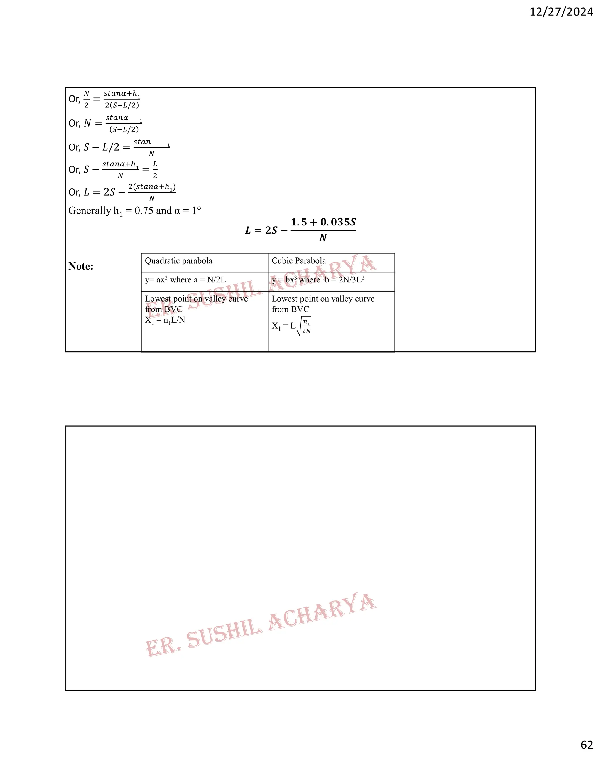
This is the equation for length of valley curve. Generally h1 = 0.75m and α = 1°
𝐿 =
𝑁𝑠2
2[0.75 + 𝑠𝑡𝑎𝑛1]
𝐿 =
𝑁𝑠2
2[0.75 + 0.0175]
𝑳 =
𝑵𝒔𝟐
𝟐[𝟏. 𝟓 + 𝟎. 𝟎𝟑𝟓𝟓]
Case b: When L<SSD
In this case the sight distance is minimum when the vehicle is at
the beginning of the valley curve.
In ∆CED
𝑡𝑎𝑛
𝑁
2
=
𝑠𝑡𝑎𝑛𝛼 + ℎ1
2
𝑆 − 𝐿/2
Or, 𝑡𝑎𝑛 =
/
here tan ≈

62. 12/27/2024
62
Or, =
/
Or, 𝑁 =
/
Or, 𝑆 − 𝐿/2 =
Or, 𝑆 − =
Or, 𝐿 = 2𝑆 −
( )
Generally h1 = 0.75 and α = 1°
𝑳 = 𝟐𝑺 −
𝟏. 𝟓 + 𝟎. 𝟎𝟑𝟓𝑺
𝑵
Note:
Cubic Parabola
Quadratic parabola
y = bx3 where b = 2N/3L2
y= ax2 where a = N/2L
Lowest point on valley curve
from BVC
X1 = L
Lowest point on valley curve
from BVC
X1 = n1L/N