Downloaded 101 times

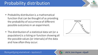
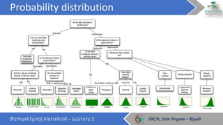


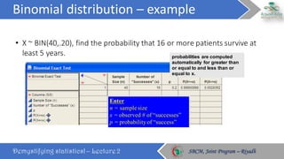
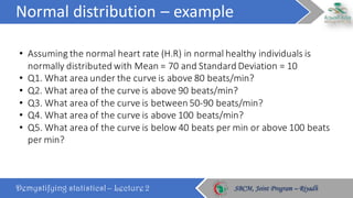
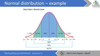

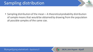
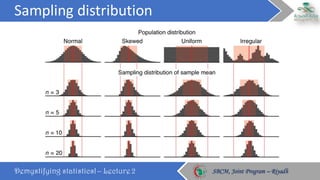
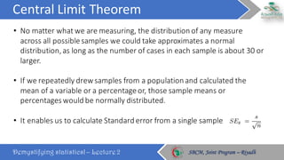

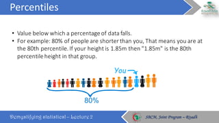
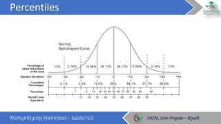


This document discusses key concepts in probability distributions including binomial, normal, and sampling distributions. It begins by defining probability distributions and listing common types. Key points about the binomial distribution are outlined including properties and an example. The normal distribution is then described in detail along with its properties and an example calculation. Sampling distributions and the central limit theorem are also introduced. The document concludes by defining percentiles and quantiles.