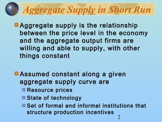
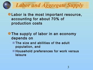
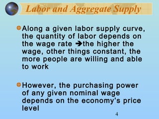
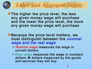
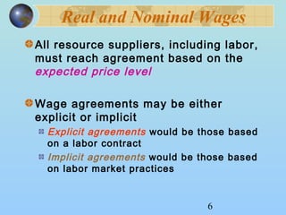
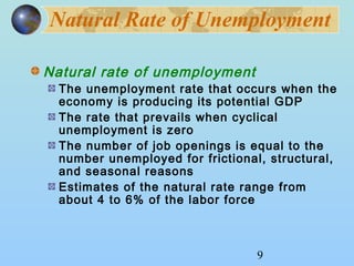
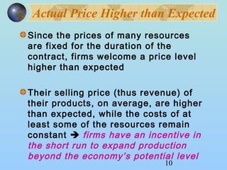
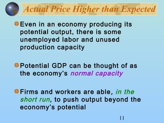
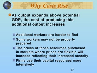
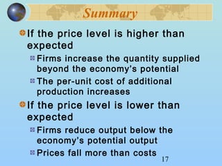
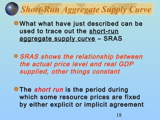
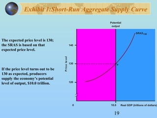
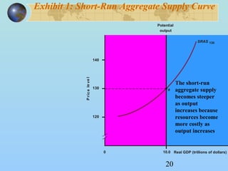
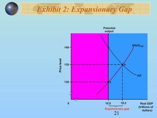
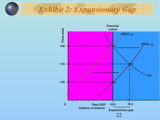
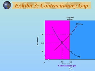
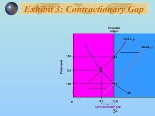
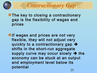
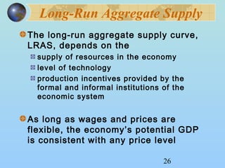
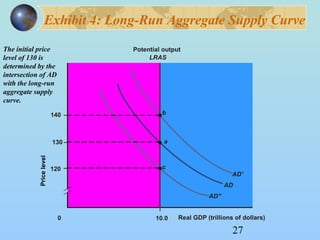
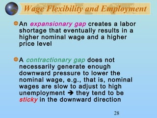
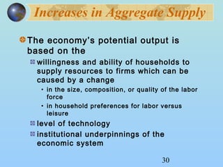
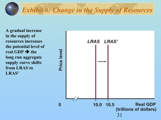
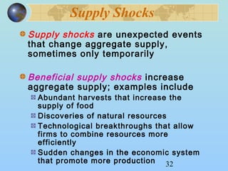
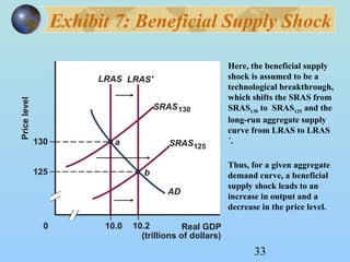
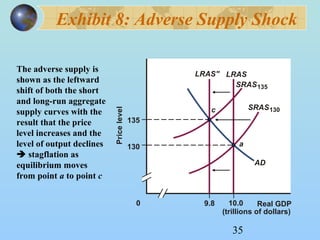
Aggregate Supply 
1 
CHAPTER 
11 
© 2003 South-Western/Thomson Learning
Aggregate Supply in Short Run 
Aggregate supply is the relationship 
between the price level in the economy 
and the aggregate output firms are 
willing and able to supply, with other 
things constant 
Assumed constant along a given 
aggregate supply curve are 
Resource prices 
State of technology 
Set of formal and informal institutions that 
structure production incentives 
2
Labor and Aggregate Supply 
Labor is the most important resource, 
accounting for about 70% of 
production costs 
The supply of labor in an economy 
depends on 
The size and abilities of the adult 
population, and 
Household preferences for work versus 
leisure 
3
Labor and Aggregate Supply 
Along a given labor supply curve, 
the quantity of labor depends on 
the wage rate the higher the 
wage, other things constant, the 
more people are willing and able 
to work 
However, the purchasing power 
of any given nominal wage 
depends on the economy’s price 
level 
4
Labor and Aggregate Supply 
The higher the price level, the less 
any given money wage will purchase 
and the lower the price level, the more 
any given money wage will purchase 
Because the price level matters, we 
must distinguish between the nominal 
wage and the real wage 
Nominal wage measures the wage in 
current dollars 
Real wage measures the wage in constant 
dollars  dollars measured by the goods 
and services they will buy 
5
Real and Nominal Wages 
All resource suppliers, including labor, 
must reach agreement based on the 
expected price level 
Wage agreements may be either 
explicit or implicit 
Explicit agreements would be those based 
on a labor contract 
Implicit agreements would be those based 
on labor market practices 
6
Potential Output 
If these price-level expectations 
are realized, the agreed-upon 
nominal wage translates into the 
expected real wage 
When the actual price level turns 
out as expected, the resulting 
level of output is referred to as 
the economy’s potential output 
Potential output is the amount 
produced when there are no 
surprises associated with the price 
level 
7
8 
Potential Output 
Potential output can be thought of as 
the economy’s maximum sustainable 
output level, given the 
Supply of resources 
State of technology 
Formal and informal production incentives 
Often referred to by other terms 
Natural rate of output 
Full-employment rate of output
Natural Rate of Unemployment 
Natural rate of unemployment 
The unemployment rate that occurs when the 
economy is producing its potential GDP 
The rate that prevails when cyclical 
unemployment is zero 
The number of job openings is equal to the 
number unemployed for frictional, structural, 
and seasonal reasons 
Estimates of the natural rate range from 
about 4 to 6% of the labor force 
9
Actual Price Higher than Expected 
Since the prices of many resources 
are fixed for the duration of the 
contract, firms welcome a price level 
higher than expected 
Their selling price (thus revenue) of 
their products, on average, are higher 
than expected, while the costs of at 
least some of the resources remain 
constant  firms have an incentive in 
the short run to expand production 
beyond the economy’s potential level 
10
Actual Price Higher than Expected 
Even in an economy producing its 
potential output, there is some 
unemployed labor and unused 
production capacity 
Potential GDP can be thought of as 
the economy’s normal capacity 
Firms and workers are able, in the 
short run, to push output beyond the 
economy’s potential 
11
12 
Why Costs Rise 
As output expands above potential 
GDP, the cost of producing this 
additional output increases 
Additional workers are harder to find 
Some workers may not be properly 
prepared 
The prices of those resources purchased 
in markets where prices are flexible will 
increase reflecting their increased scarcity 
Firms use their capital resources more 
intensively
13 
Why Costs Rise 
However, because the prices of some 
resources are fixed by contracts, the 
price level rises faster than the per-unit 
production cost  firms find it 
profitable to increase the quantity 
supplied 
When the actual price level exceeds 
the expected price level, the real value 
of an agreed-upon nominal wage 
declines
14 
Summary 
If the price level is higher than expected, 
firms have a profit incentive to increase 
the quantity of goods and services 
supplied 
At higher rates of output, however, the 
per-unit cost of additional output 
increases 
Firms will expand output as long as the 
revenue from additional production 
exceeds the cost of the production
Actual Price Lower than Expected 
Production is less attractive to firms 
because the prices they receive for their 
output are on average lower than they 
expected 
However, many of their production costs, 
such as the nominal wage, do not fall  
production is less profitable than 
expected  firms reduce their quantity 
supplied  the economy’s output is 
below its potential 
15
Actual Price Lower than Expected 
As a result, some workers are 
laid off and capital resources go 
unused 
In this case, some costs decline 
when output falls below the 
economy’s potential 
As output falls, some resources 
become unemployed 
16
17 
Summary 
If the price level is higher than 
expected 
Firms increase the quantity supplied 
beyond the economy’s potential 
The per-unit cost of additional 
production increases 
If the price level is lower than 
expected 
Firms reduce output below the 
economy’s potential output 
Prices fall more than costs
Short-Run Aggregate Supply Curve 
What what have just described can be 
used to trace out the short-run 
aggregate supply curve – SRAS 
SRAS shows the relationship between 
the actual price level and real GDP 
supplied, other things constant 
The short run is the period during 
which some resource prices are fixed 
by either explicit or implicit agreement 
18
Exhibit 1:Short-Run Aggregate Supply Curve 
a 
19 
Price level 
140 
130 
120 
Potential 
output 
SRAS130 
0 10.0 Real GDP (trillions of dollars) 
The expected price level is 130; 
the SRAS is based on that 
expected price level. 
If the price level turns out to be 
130 as expected, producers 
supply the economy’s potential 
level of output, $10.0 trillion.
Exhibit 1: Short-Run Aggregate Supply Curve 
a 
20 
P ric e le ve l 
140 
130 
120 
Potential 
output 
SRAS 130 
The short-run 
aggregate supply 
becomes steeper 
as output 
increases because 
resources become 
more costly as 
output increases 
0 10.0 R eal GDP (trillions of dollars)
Exhibit 2: Expansionary Gap 
21 
output 
a 
130 
Potential 
SRAS 130 
0 10.0 Real GDP 
(trillions of 
dollars) 
Price level 
140 
Expansionary gap 
135 
AD 
b 
10.2
Exhibit 2: Expansionary Gap 
output 
22 
c 
a 
130 
Potential 
0 R e a l G D P 10.0 
(trillions of dollars) 
SRAS 130 
Price level 
140 
SRAS 140 
Expansionary gap 
135 
AD 
b 
10.2
Exhibit 3: Contractionary Gap 
23 
130 
Potential 
output 
d 
0 10.0 
SRAS130 
Price level 
a 
Contractionary gap 
125 
9.8 
AD 
120 e
Exhibit 3: Contractionary Gap 
24 
130 
Potential 
output 
d 
0 10.0 
SRAS130 
Price level 
a 
Contractionary gap 
125 
9.8 
AD 
SRAS120 
120 e
Contractionary Gap 
The key to closing a contractionary 
gap is the flexibility of wages and 
prices 
If wages and prices are not very 
flexible, they will not adjust very 
quickly to a contractionary gap  
shifts in the short-run aggregate 
supply curve may occur slowly  the 
economy can be stuck at an output 
and employment level below its 
potential 
25
Long-Run Aggregate Supply 
The long-run aggregate supply curve, 
LRAS, depends on the 
supply of resources in the economy 
level of technology 
production incentives provided by the 
formal and informal institutions of the 
economic system 
As long as wages and prices are 
flexible, the economy’s potential GDP 
is consistent with any price level 
26
Exhibit 4: Long-Run Aggregate Supply Curve 
AD 
27 
The initial price 
level of 130 is 
determined by the 
intersection of AD 
with the long-run 
aggregate supply 
curve. 
130 
Potential output 
LRAS 
a 
c 
0 Real GDP (trillions of dollars) 
10.0 
AD'' 
120 
b 
AD' 
140 
Price level
Wage Flexibility and Employment 
An expansionary gap creates a labor 
shortage that eventually results in a 
higher nominal wage and a higher 
price level 
A contractionary gap does not 
necessarily generate enough 
downward pressure to lower the 
nominal wage, e.g., that is, nominal 
wages are slow to adjust to high 
unemployment  they tend to be 
sticky in the downward direction 
28
Wage Flexibility and Employment 
However, an actual decline in the 
nominal wage is not necessary to 
close a contractionary gap 
All that is needed is a fall in the real 
wage 
The real wage will fall as long as the 
price level increases more than the 
nominal wage 
29
Increases in Aggregate Supply 
The economy’s potential output is 
based on the 
willingness and ability of households to 
supply resources to firms which can be 
caused by a change 
• in the size, composition, or quality of the labor 
force 
• in household preferences for labor versus 
leisure 
level of technology 
institutional underpinnings of the 
economic system 
30
Exhibit 6: Change in the Supply of Resources 
LRAS LRAS' 
31 
Price level 
0 10.0 10.5 Real GDP 
(trillions of dollars) 
A gradual increase 
in the supply of 
resources increases 
the potential level of 
real GDP  the 
long run aggregate 
supply curve shifts 
from LRAS to 
LRAS'
32 
Supply Shocks 
Supply shocks are unexpected events 
that change aggregate supply, 
sometimes only temporarily 
Beneficial supply shocks increase 
aggregate supply; examples include 
Abundant harvests that increase the 
supply of food 
Discoveries of natural resources 
Technological breakthroughs that allow 
firms to combine resources more 
efficiently 
Sudden changes in the economic system 
that promote more production
Exhibit 7: Beneficial Supply Shock 
33 
LRAS 
LRAS' 
0 10.0 Real GDP 
(trillions of dollars) 
130 
AD 
a 
SRAS130 
10.2 
125 
SRAS125 
b 
Here, the beneficial supply 
shock is assumed to be a 
technological breakthrough, 
which shifts the SRAS from 
SRAS130 to SRAS125 and the 
long-run aggregate supply 
curve from LRAS to LRAS 
´. 
Thus, for a given aggregate 
demand curve, a beneficial 
supply shock leads to an 
increase in output and a 
decrease in the price level. 
Price level
Decreases in Aggregate Supply 
Adverse supply shocks are sudden, 
unexpected events that reduce 
aggregate supply, again sometimes, 
only temporarily 
Drought could reduce the supply of a 
variety of resources 
Government instability 
Terrorist attacks 
34
Exhibit 8: Adverse Supply Shock 
35 
Price level 
LRAS 
10.0 
0 Real GDP 
(trillions of dollars) 
130 
SRAS130 
AD 
a 
135 
LRAS'' 
SRAS135 
c 
9.8 
The adverse supply is 
shown as the leftward 
shift of both the short 
and long-run aggregate 
supply curves with the 
result that the price 
level increases and the 
level of output declines 
 stagflation as 
equilibrium moves 
from point a to point c

Chapter 11 (1)

  • 1.
    Aggregate Supply 1 CHAPTER 11 © 2003 South-Western/Thomson Learning
  • 2.
    Aggregate Supply inShort Run Aggregate supply is the relationship between the price level in the economy and the aggregate output firms are willing and able to supply, with other things constant Assumed constant along a given aggregate supply curve are Resource prices State of technology Set of formal and informal institutions that structure production incentives 2
  • 3.
    Labor and AggregateSupply Labor is the most important resource, accounting for about 70% of production costs The supply of labor in an economy depends on The size and abilities of the adult population, and Household preferences for work versus leisure 3
  • 4.
    Labor and AggregateSupply Along a given labor supply curve, the quantity of labor depends on the wage rate the higher the wage, other things constant, the more people are willing and able to work However, the purchasing power of any given nominal wage depends on the economy’s price level 4
  • 5.
    Labor and AggregateSupply The higher the price level, the less any given money wage will purchase and the lower the price level, the more any given money wage will purchase Because the price level matters, we must distinguish between the nominal wage and the real wage Nominal wage measures the wage in current dollars Real wage measures the wage in constant dollars  dollars measured by the goods and services they will buy 5
  • 6.
    Real and NominalWages All resource suppliers, including labor, must reach agreement based on the expected price level Wage agreements may be either explicit or implicit Explicit agreements would be those based on a labor contract Implicit agreements would be those based on labor market practices 6
  • 7.
    Potential Output Ifthese price-level expectations are realized, the agreed-upon nominal wage translates into the expected real wage When the actual price level turns out as expected, the resulting level of output is referred to as the economy’s potential output Potential output is the amount produced when there are no surprises associated with the price level 7
  • 8.
    8 Potential Output Potential output can be thought of as the economy’s maximum sustainable output level, given the Supply of resources State of technology Formal and informal production incentives Often referred to by other terms Natural rate of output Full-employment rate of output
  • 9.
    Natural Rate ofUnemployment Natural rate of unemployment The unemployment rate that occurs when the economy is producing its potential GDP The rate that prevails when cyclical unemployment is zero The number of job openings is equal to the number unemployed for frictional, structural, and seasonal reasons Estimates of the natural rate range from about 4 to 6% of the labor force 9
  • 10.
    Actual Price Higherthan Expected Since the prices of many resources are fixed for the duration of the contract, firms welcome a price level higher than expected Their selling price (thus revenue) of their products, on average, are higher than expected, while the costs of at least some of the resources remain constant  firms have an incentive in the short run to expand production beyond the economy’s potential level 10
  • 11.
    Actual Price Higherthan Expected Even in an economy producing its potential output, there is some unemployed labor and unused production capacity Potential GDP can be thought of as the economy’s normal capacity Firms and workers are able, in the short run, to push output beyond the economy’s potential 11
  • 12.
    12 Why CostsRise As output expands above potential GDP, the cost of producing this additional output increases Additional workers are harder to find Some workers may not be properly prepared The prices of those resources purchased in markets where prices are flexible will increase reflecting their increased scarcity Firms use their capital resources more intensively
  • 13.
    13 Why CostsRise However, because the prices of some resources are fixed by contracts, the price level rises faster than the per-unit production cost  firms find it profitable to increase the quantity supplied When the actual price level exceeds the expected price level, the real value of an agreed-upon nominal wage declines
  • 14.
    14 Summary Ifthe price level is higher than expected, firms have a profit incentive to increase the quantity of goods and services supplied At higher rates of output, however, the per-unit cost of additional output increases Firms will expand output as long as the revenue from additional production exceeds the cost of the production
  • 15.
    Actual Price Lowerthan Expected Production is less attractive to firms because the prices they receive for their output are on average lower than they expected However, many of their production costs, such as the nominal wage, do not fall  production is less profitable than expected  firms reduce their quantity supplied  the economy’s output is below its potential 15
  • 16.
    Actual Price Lowerthan Expected As a result, some workers are laid off and capital resources go unused In this case, some costs decline when output falls below the economy’s potential As output falls, some resources become unemployed 16
  • 17.
    17 Summary Ifthe price level is higher than expected Firms increase the quantity supplied beyond the economy’s potential The per-unit cost of additional production increases If the price level is lower than expected Firms reduce output below the economy’s potential output Prices fall more than costs
  • 18.
    Short-Run Aggregate SupplyCurve What what have just described can be used to trace out the short-run aggregate supply curve – SRAS SRAS shows the relationship between the actual price level and real GDP supplied, other things constant The short run is the period during which some resource prices are fixed by either explicit or implicit agreement 18
  • 19.
    Exhibit 1:Short-Run AggregateSupply Curve a 19 Price level 140 130 120 Potential output SRAS130 0 10.0 Real GDP (trillions of dollars) The expected price level is 130; the SRAS is based on that expected price level. If the price level turns out to be 130 as expected, producers supply the economy’s potential level of output, $10.0 trillion.
  • 20.
    Exhibit 1: Short-RunAggregate Supply Curve a 20 P ric e le ve l 140 130 120 Potential output SRAS 130 The short-run aggregate supply becomes steeper as output increases because resources become more costly as output increases 0 10.0 R eal GDP (trillions of dollars)
  • 21.
    Exhibit 2: ExpansionaryGap 21 output a 130 Potential SRAS 130 0 10.0 Real GDP (trillions of dollars) Price level 140 Expansionary gap 135 AD b 10.2
  • 22.
    Exhibit 2: ExpansionaryGap output 22 c a 130 Potential 0 R e a l G D P 10.0 (trillions of dollars) SRAS 130 Price level 140 SRAS 140 Expansionary gap 135 AD b 10.2
  • 23.
    Exhibit 3: ContractionaryGap 23 130 Potential output d 0 10.0 SRAS130 Price level a Contractionary gap 125 9.8 AD 120 e
  • 24.
    Exhibit 3: ContractionaryGap 24 130 Potential output d 0 10.0 SRAS130 Price level a Contractionary gap 125 9.8 AD SRAS120 120 e
  • 25.
    Contractionary Gap Thekey to closing a contractionary gap is the flexibility of wages and prices If wages and prices are not very flexible, they will not adjust very quickly to a contractionary gap  shifts in the short-run aggregate supply curve may occur slowly  the economy can be stuck at an output and employment level below its potential 25
  • 26.
    Long-Run Aggregate Supply The long-run aggregate supply curve, LRAS, depends on the supply of resources in the economy level of technology production incentives provided by the formal and informal institutions of the economic system As long as wages and prices are flexible, the economy’s potential GDP is consistent with any price level 26
  • 27.
    Exhibit 4: Long-RunAggregate Supply Curve AD 27 The initial price level of 130 is determined by the intersection of AD with the long-run aggregate supply curve. 130 Potential output LRAS a c 0 Real GDP (trillions of dollars) 10.0 AD'' 120 b AD' 140 Price level
  • 28.
    Wage Flexibility andEmployment An expansionary gap creates a labor shortage that eventually results in a higher nominal wage and a higher price level A contractionary gap does not necessarily generate enough downward pressure to lower the nominal wage, e.g., that is, nominal wages are slow to adjust to high unemployment  they tend to be sticky in the downward direction 28
  • 29.
    Wage Flexibility andEmployment However, an actual decline in the nominal wage is not necessary to close a contractionary gap All that is needed is a fall in the real wage The real wage will fall as long as the price level increases more than the nominal wage 29
  • 30.
    Increases in AggregateSupply The economy’s potential output is based on the willingness and ability of households to supply resources to firms which can be caused by a change • in the size, composition, or quality of the labor force • in household preferences for labor versus leisure level of technology institutional underpinnings of the economic system 30
  • 31.
    Exhibit 6: Changein the Supply of Resources LRAS LRAS' 31 Price level 0 10.0 10.5 Real GDP (trillions of dollars) A gradual increase in the supply of resources increases the potential level of real GDP  the long run aggregate supply curve shifts from LRAS to LRAS'
  • 32.
    32 Supply Shocks Supply shocks are unexpected events that change aggregate supply, sometimes only temporarily Beneficial supply shocks increase aggregate supply; examples include Abundant harvests that increase the supply of food Discoveries of natural resources Technological breakthroughs that allow firms to combine resources more efficiently Sudden changes in the economic system that promote more production
  • 33.
    Exhibit 7: BeneficialSupply Shock 33 LRAS LRAS' 0 10.0 Real GDP (trillions of dollars) 130 AD a SRAS130 10.2 125 SRAS125 b Here, the beneficial supply shock is assumed to be a technological breakthrough, which shifts the SRAS from SRAS130 to SRAS125 and the long-run aggregate supply curve from LRAS to LRAS ´. Thus, for a given aggregate demand curve, a beneficial supply shock leads to an increase in output and a decrease in the price level. Price level
  • 34.
    Decreases in AggregateSupply Adverse supply shocks are sudden, unexpected events that reduce aggregate supply, again sometimes, only temporarily Drought could reduce the supply of a variety of resources Government instability Terrorist attacks 34
  • 35.
    Exhibit 8: AdverseSupply Shock 35 Price level LRAS 10.0 0 Real GDP (trillions of dollars) 130 SRAS130 AD a 135 LRAS'' SRAS135 c 9.8 The adverse supply is shown as the leftward shift of both the short and long-run aggregate supply curves with the result that the price level increases and the level of output declines  stagflation as equilibrium moves from point a to point c