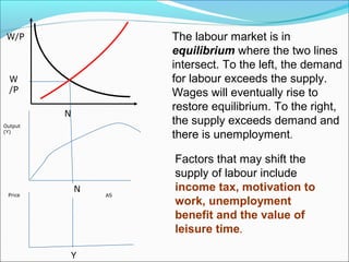
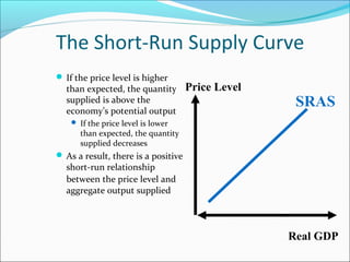
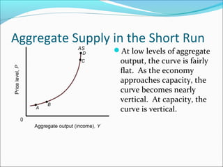
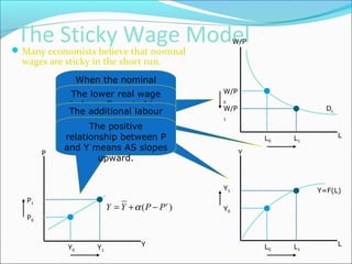
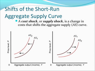
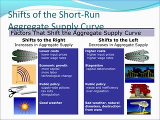
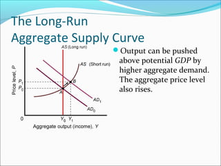
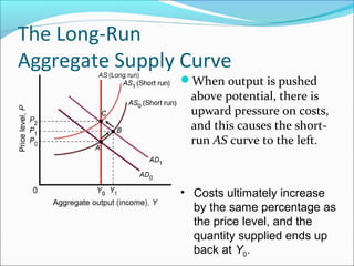
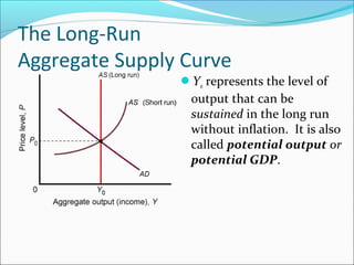
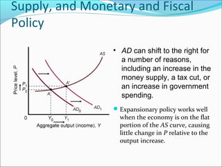
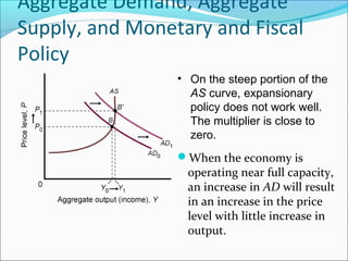
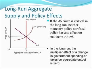
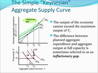
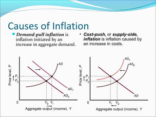
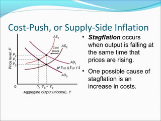
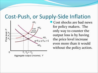
Aggregate Supply
 Aggregate supply is the relationship between the price level in the

economy and the quantity of aggregate output firms are willing
and able to supply, other things held constant
 The foundation of aggregate supply is the labor market

 Like any market, the labor market has a demand side and a supply side
 A good understanding of aggregate supply requires a correct

understanding of the demand and supply sides of the labor market
The Aggregate Supply Curve:
A Warning
The aggregate supply curve is not

a market supply curve or the sum
of all the individual supply curves
in the economy.
 The Aggregate Supply (AS) curve is an important tool in analysing

the macroeconomy. Its shape describes whether and by how
much an economy can increase output.
 The curve is built from and affected by some of the main
macroeconomic building blocks such as wages, labour and
prices and production function.
 The curve can be used to analyses the effect of changes in these
on the economy as a whole, and to examine the impact of shocks
such as oil shocks. Both long and short run effects need to be
considered.
 A detailed understanding is required to understand the shape of
AS CURVE
The Aggregate Supply curve is derived ultimately from the short run aggregate
production function.
A production function is a mathematical relationship between inputs and outputs.
At the macroeconomic level, the aggregate production function shows the
relationship between Gross Domestic Product, GDP (Y), and various
macroeconomic inputs. The most important of these are the hours of labour
employed (N) and the units of capital employed (K), all though others such as
the price of oil or technology may be relevant if these change. This then gives a
production function:
Y=
f(N,K)

where f is the aggregate production function. Note that Y always
increases if one of the inputs increases (monotonically
increasing). Increasing all units by an equal proportion (e.g.
doubling) will increase Y by the same proportion (constant returns
to scale), but the curve will exhibit diminishing marginal returns.
Assuming Capital is

constant
Y= F(N)
National Y increases
with increase in N
But at a diminishing
rate
Demand Theory states
that Entrepreneurs
employ till
MPL*P=W
W/P= MPL
In capitalist economies, firms will only employ the labour (and
other inputs) that they need to. This makes the demand for
labour, the Marginal Productivity of Labour (MPL), a derived
demand.
This function can be worked out from the slope of the short run
aggregate production function. Mathematically speaking, MPL is
the first derivative, δf/δN, of Y=f(N,K¯),
where w is nominal wages, p is the price level and w/p is real
wages. This is shifted by the same factors as Y=f(N,K¯), such
as improvements in technology or increase in capital.
In the short run, we can consider K to be fixed ( ). The short

run aggregate production function is then Y=f(N, ),
Varying N will cause a move along the curve, whilst varying K
(or any other input) will shift the curve up or down.
Y=f(N, )
w
p
MPL
In capitalist economies, firms will only employ the labour (and
other inputs) that they need to. This makes the demand for
labour, the Marginal Productivity of Labour (MPL), a
derived demand.
This function can be worked out from the slope of the short
run aggregate production function. Mathematically speaking,
MPL is the first derivative, δf/δN, of Y=f(N,K¯),
where w is nominal wages, p is the price level and w/p is
real wages. This is shifted by the same factors as Y=f(N,K¯),
such as improvements in technology or increase in capital.
The Nominal Wage and the Real
Wage
The nominal wage is the wage measured in terms of

current dollars
The real wage is the wage measured in terms of dollars
of constant purchasing power
 The real wage is the wage measured in terms of the quantity of

goods it will purchase

Both workers and employers care more about the real

wage than the nominal wage
Wages and Price Level
Expectations
 Nominal wages are

important because
resource agreements (such
as wage contracts) are
typically negotiated in
nominal wages
 Since wage contracts are
negotiated ahead of time,
they are based on workers’
expectation for the price
level



Y=f(N,K )

Y
w0
p0

w1
p1



N0

N

MPL

N1

N

N0

N1
Labor Supply
 The supply of labor depends

primarily on the wage rate
(the dollar cost of a unit of
labor, such as an hour of
work)
 The supply of labor also
depends on
 The size of the adult

population
 The skills (productivity) of
the adult population
 Households’ preferences for
work versus leisure

w0
p0

w1
p1

N0

N1
The labour market is in
equilibrium where the two lines
intersect. To the left, the demand
for labour exceeds the supply.
Wages will eventually rise to
restore equilibrium. To the right,
the supply exceeds demand and
there is unemployment.

W/P

W
/P
N
Output
(Y)

Price

N

Y

AS

Factors that may shift the
supply of labour include
income tax, motivation to
work, unemployment
benefit and the value of
leisure time.
Potential Output and the Natural Rate of
Unemployment
Potential output is the economy’s maximum

sustainable output level, given the supply of
resources, technology, and the underlying
economic institutions.
Another point of view is the that potential output is
the level of output where there are no “surprises”
about the price level.
The natural rate of unemployment is the rate that
occurs when the economy is producing it potential
level of output
Aggregate Supply in the Short Run
Macroeconomists focus on whether or not the

economy as a whole is operating at full
capacity.
As the economy approaches maximum
capacity, firms respond to further increases in
demand only by raising prices.

Hence The Classical Aggregate supply curve is

a vertical line

In long run when all resources are completely

employed then firms respond to increase in
demand by raising prices
The Aggregate Supply Curve:
A Warning
When we draw a firm’s supply curve, we

assume that input prices are constant. In
macroeconomics, an increase in the
overall price level means that at least
some input prices will be rising as well.
The outputs of some firms are the inputs
of other firms.
The Aggregate Supply Curve:
A Warning
Rather than an aggregate supply curve, what

does exist is a “price/output response” curve —
a curve that traces out the price and output
decisions of all the markets and firms in the
economy under a given set of circumstances.
Keynesian Aggregate supply Model

Keynes assumed that input prices in short run are

not flexible ,
At less than full employment level increase in AD
leads to rise in output without increase in wages or
input prices
AS

P

Y
The Short Run
The short run is a

period during which
some resources prices,
especially labor, are
fixed by agreement
The Short-Run Supply Curve
 If the price level is higher

than expected, the quantity
supplied is above the
economy’s potential output

Price Level

SRAS

 If the price level is lower

than expected, the quantity
supplied decreases

 As a result, there is a positive

short-run relationship
between the price level and
aggregate output supplied

Real GDP
Aggregate Supply in the Short Run
At low levels of aggregate

output, the curve is fairly
flat. As the economy
approaches capacity, the
curve becomes nearly
vertical. At capacity, the
curve is vertical.
The Sticky Wage Model
W/P

 Many economists believe that nominal

wages are sticky in the short run.

P

When the nominal
wage lower real wage
The is stuck, a rise in
P from P0 to P1to hire
induces firms lowers
The more labour.
additional labour
the real wage, making
hired produces more
labourpositive
The cheaper.
output.
relationship between P
and Y means AS slopes
upward.

W/P
0

W/P

DL

1

L0

L1

Y

Y1
P1

Y = Y + α (P − Pe )

P0

Y0

Y1

Y

L

Y=F(L)

Y0

L0

L1

L
Output Levels and
Price/Output Responses
When the economy is operating at low levels of

output, an increase in aggregate demand is likely to
result in an increase in output with no increase in the
overall price level. (Keynesian AS Curve )
The Response of Input Prices to
Changes in the Overall Price Level
There must be a lag between

changes in input prices and
changes in output prices,
otherwise the aggregate supply
(price/output response) curve
would be vertical.
The Long-Run
Aggregate Supply Curve
Costs lag behind price-

level changes in the short
run, resulting in an
upward-sloping AS curve.

• Costs and the price level
move in tandem in the long
run, and the AS curve is
vertical.
Shifts of the Short-Run
Aggregate Supply Curve

A cost shock, or supply shock, is a change in

costs that shifts the aggregate supply (AS) curve.
Factors That Shift the Aggregate Supply Curve
Shifts to the Right

Increases in Aggregate Supply

Shifts to the Left

Decreases in Aggregate Supply

Lower costs
lower input prices
lower wage rates

Higher costs
higher input prices
higher wage rates

Economic growth
more capital
more labor
technological change

Stagnation
capital deterioration

Public policy
supply-side policies
tax cuts
deregulation

Public policy
waste and inefficiency
over-regulation

Good weather

Bad weather, natural
disasters, destruction
from wars
The Long-Run
Aggregate Supply Curve
Output can be pushed

above potential GDP by
higher aggregate demand.
The aggregate price level
also rises.
The Long-Run
Aggregate Supply Curve
When output is pushed

above potential, there is
upward pressure on costs,
and this causes the shortrun AS curve to the left.

• Costs ultimately increase
by the same percentage as
the price level, and the
quantity supplied ends up
back at Y0.
The Long-Run
Aggregate Supply Curve
Y0 represents the level of

output that can be
sustained in the long run
without inflation. It is also
called potential output or
potential GDP.
Supply, and Monetary and Fiscal
Policy
• AD can shift to the right for
a number of reasons,
including an increase in the
money supply, a tax cut, or
an increase in government
spending.
 Expansionary policy works well

when the economy is on the flat
portion of the AS curve, causing
little change in P relative to the
output increase.
Aggregate Demand, Aggregate
Supply, and Monetary and Fiscal
Policy
• On the steep portion of the
AS curve, expansionary
policy does not work well.
The multiplier is close to
zero.
When the economy is

operating near full capacity,
an increase in AD will result
in an increase in the price
level with little increase in
output.
Long-Run Aggregate
Supply and Policy Effects
If the AS curve is vertical in

the long run, neither
monetary policy nor fiscal
policy has any effect on
aggregate output.

• In the long run, the
multiplier effect of a change
in government spending or
taxes on aggregate output
is zero.
The Simple “Keynesian”
Aggregate Supply Curve
The output of the economy

cannot exceed the maximum
output of YF.

The difference between

planned aggregate
expenditure and aggregate
output at full capacity is
sometimes referred to as an
inflationary gap.
Causes of Inflation
Inflation is an increase in the

overall price level.
Sustained inflation occurs when
the overall price level continues to
rise over some fairly long period of
time.
Causes of Inflation

• Cost-push, or supply-side,
inflation is inflation caused by
inflation initiated by an
an increase in costs.
increase in aggregate demand.

Demand-pull inflation is
Cost-Push, or Supply-Side Inflation
• Stagflation occurs
when output is falling at
the same time that
prices are rising.
• One possible cause of
stagflation is an
increase in costs.
Cost-Push, or Supply-Side Inflation
Cost shocks are bad news

for policy makers. The
only way to counter the
output loss is by having
the price level increase
even more than it would
without the policy action.
Expectations and Inflation

If every firm expects every other firm to raise

prices by 10%, every firm will raise prices by
about 10%. This is how expectations can get
“built into the system.”

• In terms of the AD/AS diagram, an
increase in inflationary expectations
shifts the AS curve to the left.
Money and Inflation

Hyperinflation is a

period of very rapid
increases in the price
level.
Money and Inflation

• An increase in G with
the money supply
constant shifts the AD
curve from AD0 to AD1.
This leads to an
increase in the interest
rate and crowding out
of planned investment.
Money and Inflation

• If the Fed tries to prevent
crowding, it will increase
the money supply and
the AD curve will shift
farther and farther to the
right. The result is a
sustained inflation,
perhaps hyperinflation.

Great introduction to as curve

  • 2.
    Aggregate Supply  Aggregatesupply is the relationship between the price level in the economy and the quantity of aggregate output firms are willing and able to supply, other things held constant  The foundation of aggregate supply is the labor market  Like any market, the labor market has a demand side and a supply side  A good understanding of aggregate supply requires a correct understanding of the demand and supply sides of the labor market
  • 3.
    The Aggregate SupplyCurve: A Warning The aggregate supply curve is not a market supply curve or the sum of all the individual supply curves in the economy.
  • 4.
     The AggregateSupply (AS) curve is an important tool in analysing the macroeconomy. Its shape describes whether and by how much an economy can increase output.  The curve is built from and affected by some of the main macroeconomic building blocks such as wages, labour and prices and production function.  The curve can be used to analyses the effect of changes in these on the economy as a whole, and to examine the impact of shocks such as oil shocks. Both long and short run effects need to be considered.  A detailed understanding is required to understand the shape of AS CURVE
  • 5.
    The Aggregate Supplycurve is derived ultimately from the short run aggregate production function. A production function is a mathematical relationship between inputs and outputs. At the macroeconomic level, the aggregate production function shows the relationship between Gross Domestic Product, GDP (Y), and various macroeconomic inputs. The most important of these are the hours of labour employed (N) and the units of capital employed (K), all though others such as the price of oil or technology may be relevant if these change. This then gives a production function: Y= f(N,K) where f is the aggregate production function. Note that Y always increases if one of the inputs increases (monotonically increasing). Increasing all units by an equal proportion (e.g. doubling) will increase Y by the same proportion (constant returns to scale), but the curve will exhibit diminishing marginal returns.
  • 6.
    Assuming Capital is constant Y=F(N) National Y increases with increase in N But at a diminishing rate Demand Theory states that Entrepreneurs employ till MPL*P=W W/P= MPL
  • 7.
    In capitalist economies,firms will only employ the labour (and other inputs) that they need to. This makes the demand for labour, the Marginal Productivity of Labour (MPL), a derived demand. This function can be worked out from the slope of the short run aggregate production function. Mathematically speaking, MPL is the first derivative, δf/δN, of Y=f(N,K¯), where w is nominal wages, p is the price level and w/p is real wages. This is shifted by the same factors as Y=f(N,K¯), such as improvements in technology or increase in capital.
  • 8.
    In the shortrun, we can consider K to be fixed ( ). The short run aggregate production function is then Y=f(N, ), Varying N will cause a move along the curve, whilst varying K (or any other input) will shift the curve up or down. Y=f(N, ) w p MPL In capitalist economies, firms will only employ the labour (and other inputs) that they need to. This makes the demand for labour, the Marginal Productivity of Labour (MPL), a derived demand. This function can be worked out from the slope of the short run aggregate production function. Mathematically speaking, MPL is the first derivative, δf/δN, of Y=f(N,K¯), where w is nominal wages, p is the price level and w/p is real wages. This is shifted by the same factors as Y=f(N,K¯), such as improvements in technology or increase in capital.
  • 9.
    The Nominal Wageand the Real Wage The nominal wage is the wage measured in terms of current dollars The real wage is the wage measured in terms of dollars of constant purchasing power  The real wage is the wage measured in terms of the quantity of goods it will purchase Both workers and employers care more about the real wage than the nominal wage
  • 10.
    Wages and PriceLevel Expectations  Nominal wages are important because resource agreements (such as wage contracts) are typically negotiated in nominal wages  Since wage contracts are negotiated ahead of time, they are based on workers’ expectation for the price level
  • 11.
  • 12.
    Labor Supply  Thesupply of labor depends primarily on the wage rate (the dollar cost of a unit of labor, such as an hour of work)  The supply of labor also depends on  The size of the adult population  The skills (productivity) of the adult population  Households’ preferences for work versus leisure w0 p0 w1 p1 N0 N1
  • 13.
    The labour marketis in equilibrium where the two lines intersect. To the left, the demand for labour exceeds the supply. Wages will eventually rise to restore equilibrium. To the right, the supply exceeds demand and there is unemployment. W/P W /P N Output (Y) Price N Y AS Factors that may shift the supply of labour include income tax, motivation to work, unemployment benefit and the value of leisure time.
  • 14.
    Potential Output andthe Natural Rate of Unemployment Potential output is the economy’s maximum sustainable output level, given the supply of resources, technology, and the underlying economic institutions. Another point of view is the that potential output is the level of output where there are no “surprises” about the price level. The natural rate of unemployment is the rate that occurs when the economy is producing it potential level of output
  • 15.
    Aggregate Supply inthe Short Run Macroeconomists focus on whether or not the economy as a whole is operating at full capacity. As the economy approaches maximum capacity, firms respond to further increases in demand only by raising prices. Hence The Classical Aggregate supply curve is a vertical line In long run when all resources are completely employed then firms respond to increase in demand by raising prices
  • 16.
    The Aggregate SupplyCurve: A Warning When we draw a firm’s supply curve, we assume that input prices are constant. In macroeconomics, an increase in the overall price level means that at least some input prices will be rising as well. The outputs of some firms are the inputs of other firms.
  • 17.
    The Aggregate SupplyCurve: A Warning Rather than an aggregate supply curve, what does exist is a “price/output response” curve — a curve that traces out the price and output decisions of all the markets and firms in the economy under a given set of circumstances.
  • 18.
    Keynesian Aggregate supplyModel Keynes assumed that input prices in short run are not flexible , At less than full employment level increase in AD leads to rise in output without increase in wages or input prices AS P Y
  • 19.
    The Short Run Theshort run is a period during which some resources prices, especially labor, are fixed by agreement
  • 20.
    The Short-Run SupplyCurve  If the price level is higher than expected, the quantity supplied is above the economy’s potential output Price Level SRAS  If the price level is lower than expected, the quantity supplied decreases  As a result, there is a positive short-run relationship between the price level and aggregate output supplied Real GDP
  • 21.
    Aggregate Supply inthe Short Run At low levels of aggregate output, the curve is fairly flat. As the economy approaches capacity, the curve becomes nearly vertical. At capacity, the curve is vertical.
  • 22.
    The Sticky WageModel W/P  Many economists believe that nominal wages are sticky in the short run. P When the nominal wage lower real wage The is stuck, a rise in P from P0 to P1to hire induces firms lowers The more labour. additional labour the real wage, making hired produces more labourpositive The cheaper. output. relationship between P and Y means AS slopes upward. W/P 0 W/P DL 1 L0 L1 Y Y1 P1 Y = Y + α (P − Pe ) P0 Y0 Y1 Y L Y=F(L) Y0 L0 L1 L
  • 23.
    Output Levels and Price/OutputResponses When the economy is operating at low levels of output, an increase in aggregate demand is likely to result in an increase in output with no increase in the overall price level. (Keynesian AS Curve )
  • 24.
    The Response ofInput Prices to Changes in the Overall Price Level There must be a lag between changes in input prices and changes in output prices, otherwise the aggregate supply (price/output response) curve would be vertical.
  • 25.
    The Long-Run Aggregate SupplyCurve Costs lag behind price- level changes in the short run, resulting in an upward-sloping AS curve. • Costs and the price level move in tandem in the long run, and the AS curve is vertical.
  • 26.
    Shifts of theShort-Run Aggregate Supply Curve A cost shock, or supply shock, is a change in costs that shifts the aggregate supply (AS) curve.
  • 27.
    Factors That Shiftthe Aggregate Supply Curve Shifts to the Right Increases in Aggregate Supply Shifts to the Left Decreases in Aggregate Supply Lower costs lower input prices lower wage rates Higher costs higher input prices higher wage rates Economic growth more capital more labor technological change Stagnation capital deterioration Public policy supply-side policies tax cuts deregulation Public policy waste and inefficiency over-regulation Good weather Bad weather, natural disasters, destruction from wars
  • 28.
    The Long-Run Aggregate SupplyCurve Output can be pushed above potential GDP by higher aggregate demand. The aggregate price level also rises.
  • 29.
    The Long-Run Aggregate SupplyCurve When output is pushed above potential, there is upward pressure on costs, and this causes the shortrun AS curve to the left. • Costs ultimately increase by the same percentage as the price level, and the quantity supplied ends up back at Y0.
  • 30.
    The Long-Run Aggregate SupplyCurve Y0 represents the level of output that can be sustained in the long run without inflation. It is also called potential output or potential GDP.
  • 31.
    Supply, and Monetaryand Fiscal Policy • AD can shift to the right for a number of reasons, including an increase in the money supply, a tax cut, or an increase in government spending.  Expansionary policy works well when the economy is on the flat portion of the AS curve, causing little change in P relative to the output increase.
  • 32.
    Aggregate Demand, Aggregate Supply,and Monetary and Fiscal Policy • On the steep portion of the AS curve, expansionary policy does not work well. The multiplier is close to zero. When the economy is operating near full capacity, an increase in AD will result in an increase in the price level with little increase in output.
  • 33.
    Long-Run Aggregate Supply andPolicy Effects If the AS curve is vertical in the long run, neither monetary policy nor fiscal policy has any effect on aggregate output. • In the long run, the multiplier effect of a change in government spending or taxes on aggregate output is zero.
  • 34.
    The Simple “Keynesian” AggregateSupply Curve The output of the economy cannot exceed the maximum output of YF. The difference between planned aggregate expenditure and aggregate output at full capacity is sometimes referred to as an inflationary gap.
  • 35.
    Causes of Inflation Inflationis an increase in the overall price level. Sustained inflation occurs when the overall price level continues to rise over some fairly long period of time.
  • 36.
    Causes of Inflation •Cost-push, or supply-side, inflation is inflation caused by inflation initiated by an an increase in costs. increase in aggregate demand. Demand-pull inflation is
  • 37.
    Cost-Push, or Supply-SideInflation • Stagflation occurs when output is falling at the same time that prices are rising. • One possible cause of stagflation is an increase in costs.
  • 38.
    Cost-Push, or Supply-SideInflation Cost shocks are bad news for policy makers. The only way to counter the output loss is by having the price level increase even more than it would without the policy action.
  • 39.
    Expectations and Inflation Ifevery firm expects every other firm to raise prices by 10%, every firm will raise prices by about 10%. This is how expectations can get “built into the system.” • In terms of the AD/AS diagram, an increase in inflationary expectations shifts the AS curve to the left.
  • 40.
    Money and Inflation Hyperinflationis a period of very rapid increases in the price level.
  • 41.
    Money and Inflation •An increase in G with the money supply constant shifts the AD curve from AD0 to AD1. This leads to an increase in the interest rate and crowding out of planned investment.
  • 42.
    Money and Inflation •If the Fed tries to prevent crowding, it will increase the money supply and the AD curve will shift farther and farther to the right. The result is a sustained inflation, perhaps hyperinflation.

Editor's Notes

  • #22 Firms may at time have excess capital and excess labor on hand. The reasons for this are associated with the costs of getting rid of capital and labor.
  • #25 If input and output prices rise by the same percentage amount, no firm would find it advantageous to change its level of output.
  • #27 Cost shocks refer to an increase in costs, which may be the result of an increase in wage rates, energy prices, natural disasters, economic stagnation, and the like.
  • #40 If prices have been rising, and if people’s expectations are adaptive—that is, if they form their expectations on the basis of past pricing behavior—then firms may continue raising prices even if demand is slowing or contracting.
  • #41 If prices have been rising, and if people’s expectations are adaptive—that is, if they form their expectations on the basis of past pricing behavior—then firms may continue raising prices even if demand is slowing or contracting.
  • #42 If prices have been rising, and if people’s expectations are adaptive—that is, if they form their expectations on the basis of past pricing behavior—then firms may continue raising prices even if demand is slowing or contracting.
  • #43 If prices have been rising, and if people’s expectations are adaptive—that is, if they form their expectations on the basis of past pricing behavior—then firms may continue raising prices even if demand is slowing or contracting.