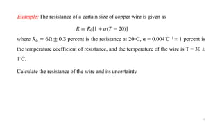
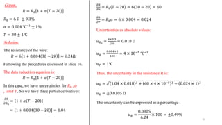
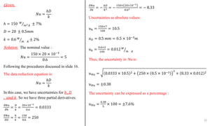
Engineering Measurements
Chapter 4: Uncertainty Analysis
Naief Almalki, PhD
1
4.1 Introduction
• Measurement is the process of assigning a value to a physical variable based on a sampling from
the population of that variable.
• Error causes a difference between the value assigned by measurement and the true value of the
population of the variable.
• Since we don’t know the true value, we only estimate the probable range of error. This estimation
is the uncertainty analysis.
• The uncertainty describes an interval about the measured value within which we suspect that the
true value must fall with a stated probability.
Errors are effects, and uncertainties are numbers!
2
4.2 Measurement Errors
3
𝑢𝑥 combines the uncertainty
estimates of the random error
and of systematic error in the
measurement of x
4.3 Combining Elemental Errors: RSS
Method
• Each individual measurement error interacts with other errors to affect the
uncertainty of a measurement. This is called uncertainty propagation.
• Each individual error is called an ‘‘elemental error.’’
• For example, the sensitivity error and linearity error of a transducer are two
elemental errors, and the numbers associated with these are their uncertainties.
4
4.3 Combining Elemental Errors: RSS
Method
• Consider a measurement of x that is subject to some K elements of error, each of
uncertainty 𝑢𝑘, where k= 1, 2, . . . ,K. A realistic estimate of the uncertainty in the
measured variable,𝑢𝑥, due to these elemental errors can be computed using the RSS
method to propagate the elemental uncertainties:
𝑢𝑥 = 𝑢1
2
+ 𝑢2
2
+ ⋯ + 𝑢𝑘
2
= ෍
𝑘=1
𝐾
𝑢𝑘
2
5
4.3 Combining Elemental Errors: RSS
Method
• In test engineering, it is common to report final uncertainties at a 95% probability
level (P%=95%), and this is equivalent to assuming the probability covered by
two standard deviations.
• When a probability level equivalent to a spread of one standard deviation is used,
this uncertainty is called the ‘‘standard’’ uncertainty.
• For a normal distribution, a standard uncertainty is a 68% probability level.
• Whatever level is used, consistency is important.
6
Example: A lab technician has just received a box of 2000
resistors. To determine the nominal resistance and tolerance,
the technician selects 10 resistors and measures their
resistances with a digital multimeter (DMM). His results are as
tabulated. Consider both random and systematic uncertainty,
what is the nominal value of the resistors and its uncertainty?
The manual for the DMM describes its calibration; possible
bias uncertainty (from temperature drift, connecting-lead
resistances, and other sources) is rated as:
±(0.5% of reading + 0.05% of full scale + 0.2 Ω)
The full scale reading of the DMM is 20 kΩ.
7
Number Resistance (k ohms)
1 18.12
2 17.95
3 18.17
4 18.45
5 16.24
6 17.82
7 16.28
8 16.32
9 17.91
10 15.98
Solution. The nominal value is the mean. The
tolerance is the uncertainty as:
𝑢𝑥 = 𝑢𝑠
2
+ 𝑢𝑟
2
The sample statistics are:
ҧ
𝑥 = 17.32 𝑘Ω
𝜎 = 0.982 𝑘Ω
The random uncertainty for a sample mean:
ƴ
𝑥 = ҧ
𝑥 ± 𝑢𝑟
𝑢𝑟 = 𝑡9,0.95 ത
𝜎
ത
𝜎 =
𝜎
𝑛
=
0.982
10
= 0.31
From t-distribution table:
𝑡9,0.95 = 2.262
Thus,
𝑢𝑟 = ± 2.262 × 0.31 = 0.701𝑘Ω 95%
The systematic uncertainty can be estimated from the giving
information in the manual as:
𝑢𝑠 =
0.5 × 17.32
100
+
0.05 × 20
100
+
0. 2
1000
𝑢𝑠 = 0.0978 𝑘Ω ≈ 0.1𝑘Ω
The total uncertainty then is:
𝑢𝑥 = 0.12 + 0.7012 = ±0.71𝑘Ω 95%
8
4.4 Design-Stage Uncertainty
• A design-stage uncertainty estimate is intended only as a guide for selecting
equipment and procedures before a test, and is never used for reporting results.
• The design-stage uncertainty, ud, for an instrument or measurement method is an
interval found by combining the systematic uncertainty with the zero-order
uncertainty:
9
4.4 Design-Stage Uncertainty
• Systematic uncertainty uc is an estimate of the expected error due to the
instrument. This information usually is provided by the manufacturer.
• Zero-order uncertainty of the instrument, u0, assumes that the variation expected in
the measured values will be only that amount due to instrument resolution and that
all other aspects of the measurement are perfectly controlled.
10
Example: Consider the force measuring instrument
described by the following catalog data. Provide an
estimate of the uncertainty attributable to this
instrument and the instrument design-stage
uncertainty.
11
Solution. An estimate of the instrument uncertainty depends on
the uncertainty assigned to each of the contributing elemental
errors of linearity, e1, and hysteresis, e2, respectively assigned as:
u1= 0.20 N u2= 0.30 N
Then, the systematic uncertainty is:
𝑢𝑐 = 0.202 + 0.302 = 0.36 𝑁
Also, the zero-order uncertainty is:
𝑢0 =
0.25
2
= 0.125 𝑁
The design-stage uncertainty is:
𝑢𝑑 = 𝑢𝑐
2 + 𝑢0
2 = 0.362 + 0.1252 = ±0.36 𝑁 (95%)
Resolution:
Range:
Linearity error:
Hysteresis error:
0.25 N
0 to 100 N
within 0.20 N over range
within 0.30 N over range
Example: A voltmeter is used to measure
the electrical output signal from a pressure
transducer. The nominal pressure is
expected to be about 3 psi. Estimate the
design-stage uncertainty in this
combination.
12
Solution. To estimate the design-stage
uncertainty, we need to estimate the
systematic and zero order uncertainties
for each instrument. The uncertainty in
the voltmeter at the design stage is given
by:
𝑢𝑑 𝑉 = 𝑢0 𝑉
2
+ 𝑢𝑐 𝑉
2
𝑢0 𝑉 = 𝑅𝑒𝑠𝑜𝑙𝑢𝑡𝑖𝑜𝑛
1
2
=
10
2
= 5 𝜇𝑉
For a nominal value of 3 psi, we expect
the voltmeter to measure 3 V since the
sensitivity is1 V/psi. Thus:
𝑢𝑐 𝑉 = 3 ×
0.001
100
= 30 𝜇𝑉
The design-stage in the voltmeter :
𝑢𝑑 𝑉 = 52 + 302 = 30.4 𝜇𝑉
Similarly, the uncertainty in the pressure
transducer at the design stage is given by:
𝑢𝑑 𝑝 = 𝑢0 𝑝
2
+ 𝑢𝑐 𝑝
2
Since resolution of the transducer is
negligible, the zero order uncertainty of the
pressure transducer, 𝑢0 𝑝 = 0
The systematic uncertainty of the pressure
transducer is:
𝑢𝑑 𝑝 = 𝑢1
2
+ 𝑢2
2
= 2.5 × 3 2 + 2 × 3 2 = 9.61 𝑚𝑉
The design-stage in the pressure transducer :
𝑢𝑑 𝑝 = 𝑢0 𝑝
2
+ 𝑢𝑐 𝑝
2
= 0 + 9.612
= 9.61 𝑚𝑉
13
Finally, ud for the combined system:
𝑢𝑑 = 𝑢𝑑 𝑉
2
+ 𝑢𝑑 𝑝
2
= 0.0304 2 + 9.61 2
𝑢𝑑 = ±9.61𝑚𝑉 (95%)
Note that essentially all of the
uncertainty is due to the transducer.
Design-stage uncertainty analysis
shows us that a better transducer, not
a better voltmeter, is needed if we
must improve the uncertainty in this
measurement!
4.5 Propagation of Uncertainty
• In many experimental situations, the final desired result is not measured directly.
• So, measurements of several variables are substituted into a data reduction
equation to obtain the desired quantity.
• As an example, suppose the density ρ of a flowing gas stream is desired.
• Ideal gas equation can be used to find density, by measuring Pressure and
Temperature.
𝑃 = 𝜌𝑅𝑇 or 𝜌 = P/RT
• How do the uncertainties in the individual measured variables P and T propagate through
the data reduction equation into the final result for ρ ?
• Concept of error propagation is introduced in relation with the errors of original
measurements.
14
4.5 Propagation of Uncertainty
• The overall uncertainty 𝑢𝑅 of the experimental result, is determined by
combining all errors to includes bias and precision limits.
• The result R is a given function of the independent variables
𝑥1, 𝑥2, 𝑥3, … … . 𝑥𝑛. Thus,
𝑅 = 𝑅 𝑥1, 𝑥2, 𝑥3, … … … . , 𝑥𝑛
Let 𝑢𝑅is the overall uncertainty, 𝑢1, 𝑢2 , 𝑢3 , … … . . , 𝑢𝑛 be the uncertainties in
the independent variables 𝑥1, 𝑥2, 𝑥3, … … … . , 𝑥𝑛 , then the overall uncertainty
can be estimated as:
𝑢𝑅 =
𝜕𝑅
𝜕𝑥1
𝑢1
2
+
𝜕𝑅
𝜕𝑥2
𝑢2
2
+
𝜕𝑅
𝜕𝑥3
𝑢3
2
+ ⋯ +
𝜕𝑅
𝜕𝑥𝑛
𝑢𝑛
2
ൗ
1
2
15
4.5 Propagation of Uncertainty
• To estimate the uncertainty to a result, the following procedures can be followed:
1. Identify the data reduction equation and calculate the nominal value.
2. Determine the partial derivatives of the data reduction equation with respect to each
variable that has an uncertainty.
3. Convert any percentage uncertainty to an absolute one for all independent variables in
the data reduction equation.
4. Apply the propagation of uncertainty general equation discussed before.
5. Express the estimated uncertainty as an absolute and percentage.
16
Example: The volume of a cylinder is to be determined from measurements of the
diameter and length as shown in Table A. If the length and diameter are measured at
four different locations by means of a micrometer with an uncertainty of ±0.5% of
the reading. Estimate the total uncertainty in the volume of the cylinder.
17
Table A. measurements of the diameter and length of a cylinder
Diameter (in.) Length (in.)
3.9920 4.4940
3.9892 4.4991
3.9961 4.5110
3.9995 4.5221
Solution. The nominal value is the mean. The tolerance is the uncertainty. This can be
written for the diameter and length measurements as:
𝑢𝑥 = 𝑢𝑠
2
+ 𝑢𝑟
2
Therefore, we need to estimate the total in the diameter and length measurements
separately and then combine both to estimate the total uncertainty in the volume
measurements .
To find the uncertainty in the volume measurements, we will follow the
procedures in slide 16. Thus, the data reduction equation is:
𝑉 =
𝜋𝐷2
4
× 𝐿
The volume of the cylinder is
𝑉 =
𝜋𝐷2
4
× 𝐿 =
𝜋3.99492
4
× 4.5066 = 56.4873 𝑖𝑛3
In this case, we have uncertainties for 𝐷 𝑎𝑛𝑑 𝐿. So we have two partial
derivatives:
𝜕𝑉
𝜕𝐷
=
2𝜋𝐷
4
× 𝐿 =
𝜋 × 3.9949
2
× 4.5066 = 28.2797
𝜕𝑉
𝜕𝐿
=
𝜋𝐷2
4
=
𝜋 × 3.99492
4
= 12.5343
Uncertainties as absolute values:
𝑢𝐷 = 0.0212
𝑢𝐿 = 0.0301
Thus, the uncertainty in the volume is:
𝑢𝑅 = 28.2797 × 0.0212 2 + 12.5343 × 0.0301 2
𝑢𝑅 = ±0.7083 𝑖𝑛3
The uncertainty can be expressed as a percentage :
𝑢𝑅 =
0.7088
56.4873
× 100 = ±1.25%
18
Parameter Diameter Length
ҧ
𝑥 3.9949 4.5066
𝜎 0.0046 0.0126
𝑣 = 𝑛 − 1 3 3
𝑡3,0.95 3.1824 3.1824
ത
𝜎 =
𝜎
𝑛
0.0023 0.0062
𝑢𝑟 = 𝑡𝑣,𝑃 ത
𝜎 0.0073 0.0200
𝑢𝑠 =
0.5 × ҧ
𝑥
100
0.0200 0.0225
𝑢𝑥 = 𝑢𝑠
2
+ 𝑢𝑟
2
0.0212 0.0301
𝑢𝑥% =
𝑢𝑥
ҧ
𝑥
× 100 0.53 0.67
Example: The resistance of a certain size of copper wire is given as
where 𝑅0 = 6Ω ± 0.3 percent is the resistance at 20◦C, α = 0.004◦C−1 ± 1 percent is
the temperature coefficient of resistance, and the temperature of the wire is T = 30 ±
1◦C.
Calculate the resistance of the wire and its uncertainty
19
G𝑖𝑣𝑒𝑛.
𝑅 = 𝑅0 1 + 𝛼 𝑇 − 20
𝑅0 = 6 Ω ± 0.3%
𝛼 = 0.004 ℃−1
± 1%
𝑇 = 30 ± 1℃
Solution.
The resistance of the wire:
𝑅 = 6 1 + 0.004 30 − 20 = 6.24Ω
Following the procedures discussed in slide 16.
The data reduction equation is:
𝑅 = 𝑅0 1 + 𝛼 𝑇 − 20
In this case, we have uncertainties for 𝑅0 , 𝛼
, 𝑎𝑛𝑑 𝑇. So we have three partial derivatives:
𝜕𝑅
𝜕𝑅0
= 1 + 𝛼 𝑇 − 20
= 1 + 0.004 30 − 20 = 1.04
𝜕𝑅
𝜕𝛼
= 𝑅0 𝑇 − 20 = 6 30 − 20 = 60
𝜕𝑅
𝜕𝑇
= 𝑅0𝛼 = 6 × 0.004 = 0.024
Uncertainties as absolute values:
𝑢𝑅0
=
6×0.3
100
= 0.018 Ω
𝑢𝛼 =
0.004×1
100
= 4 × 10⁻⁵
℃−1
𝑢𝑇 = 1℃
Thus, the uncertainty in the resistance R is:
𝑢𝑅 = 1.04 × 0.018 2 + 60 × 4 × 10−5 2 + 0.024 × 1 2
𝑢𝑅 = ±0.0305 Ω
The uncertainty can be expressed as a percentage :
𝑢𝑅 =
0.0305
6.24
× 100 = ±0.49%
20
Example: Heat transfer from a rod of diameter D immersed in a fluid can be
described by the Nusselt number, Nu= hD/k, where h is the heat-transfer coefficient
and k is the thermal conductivity of the fluid. If h can be measured within ± 7%
(95%), estimate the uncertainty in Nu as an absolute and a percentage error for the
nominal value of h = 150 W/m2-K. Let D = 20 ±0.5 mm and k =0.6 ± 2% W/m-K.
21
G𝑖𝑣𝑒𝑛.
𝑁𝑢 =
ℎ𝐷
𝑘
ℎ = 150 Τ
𝑊
𝑚2.𝑘 ± 7%
𝐷 = 20 ± 0.5𝑚𝑚
𝑘 = 0.6 ൗ
𝑊
𝑚 .𝑘
± 2%
Solution. The nominal value :
𝑁𝑢 =
150 × 20 × 10−3
0.6
= 5
Following the procedures discussed in slide 16.
The data reduction equation is:
𝑁𝑢 =
ℎ𝐷
𝑘
In this case, we have uncertainties for ℎ , 𝐷
, 𝑎𝑛𝑑 𝑘. So we have three partial derivatives:
𝜕𝑁𝑢
𝜕ℎ
=
𝐷
𝑘
=
20×10−3
0.6
= 0.0333
𝜕𝑁𝑢
𝜕𝐷
=
ℎ
𝑘
=
150
0.6
= 250
𝜕𝑁𝑢
𝜕𝑘
= −
ℎ𝐷
𝑘2 = −
150× 20×10−3
0.62 = − 8.33
Uncertainties as absolute values:
𝑢ℎ =
150×7
100
= 10.5
𝑢𝐷 = 0.5 𝑚𝑚 = 0.5 × 10⁻³𝑚
𝑢𝑘 =
0.6×2
100
= 0.012 ൗ
𝑊
𝑚 .𝑘
Thus, the uncertainty in Nu is:
𝑢𝑁𝑢 = 0.0333 × 10.5 2 + 250 × 0.5 × 10−3 2
+ 8.33 × 0.012 2
𝑢𝑁𝑢 = ±0.38
The uncertainty can be expressed as a percentage :
𝑢𝑁𝑢 =
0.38
5
× 100 = ±7.6%
22
Example: The density of air is to be determined by measuring its pressure and
temperature for insertion in the ideal-gas equation of state; that is,
𝑝 = 𝜌𝑅𝑇
The value of R for air is 287.1 J/kg-K and may be assumed exact for this
calculation. The temperature and pressure are measured as
𝑇 = 55 ± 0.4 ℃
𝑝 = 125 ± 0.5 𝑘𝑃𝑎
Determine the nominal value for the density in kg/m3 and its uncertainty as an
absolute and a percentage error.
23
Given.
𝑃 = 𝜌𝑅𝑇 → 𝜌 =
𝑃
𝑅𝑇
𝑅 = 287.1 ൗ
𝐽
𝑘𝑔.𝑘
𝑇 = 55 ± 0.4 ℃ = 55 + 273 ± 0.4 𝐾
= 328 ± 0.4 𝐾
𝑃 = 125 ± 0.5 𝑘𝑃𝑎
Solution. The nominal value :
𝜌 =
𝑃
𝑅𝑇
=
125 × 103
287.1 × 328
= 1.327 ൗ
𝑘𝑔
𝑚3
Following the procedures discussed in slide 16.
The data reduction equation is:
𝜌 =
𝑃
𝑅𝑇
In this case, we have uncertainties for
𝑃 𝑎𝑛𝑑 𝑇. So we have two partial derivatives:
𝜕𝜌
𝜕𝑃
=
1
𝑅𝑇
=
1
287.1×328
= 1.0619 × 10⁻⁵
𝜕𝜌
𝜕𝑇
= −
𝑃
𝑅𝑇2 = −
125×103
287×3282 = −4.047 × 10⁻³
Uncertainties as absolute values:
𝑢𝑃 = 0.5𝑘𝑃𝑎 = 500 𝑃𝑎
𝑢𝑇 = 0.4 𝐾
Thus, the uncertainty in 𝜌 is:
𝑢𝜌 = 1.0619 × 10−5 × 500 2 + 4.047 × 10−3 × 0.4 2
𝑢𝜌 = ±5.55 × 10⁻³ ൗ
𝑘𝑔
𝑚3
The uncertainty can be expressed as a percentage :
𝑢𝜌 =
5.55×10⁻³
1.328
× 100 = ± 0.42%
24

Ch4_Uncertainty Analysis_1(3).pdf

  • 1.
    Engineering Measurements Chapter 4:Uncertainty Analysis Naief Almalki, PhD 1
  • 2.
    4.1 Introduction • Measurementis the process of assigning a value to a physical variable based on a sampling from the population of that variable. • Error causes a difference between the value assigned by measurement and the true value of the population of the variable. • Since we don’t know the true value, we only estimate the probable range of error. This estimation is the uncertainty analysis. • The uncertainty describes an interval about the measured value within which we suspect that the true value must fall with a stated probability. Errors are effects, and uncertainties are numbers! 2
  • 3.
    4.2 Measurement Errors 3 𝑢𝑥combines the uncertainty estimates of the random error and of systematic error in the measurement of x
  • 4.
    4.3 Combining ElementalErrors: RSS Method • Each individual measurement error interacts with other errors to affect the uncertainty of a measurement. This is called uncertainty propagation. • Each individual error is called an ‘‘elemental error.’’ • For example, the sensitivity error and linearity error of a transducer are two elemental errors, and the numbers associated with these are their uncertainties. 4
  • 5.
    4.3 Combining ElementalErrors: RSS Method • Consider a measurement of x that is subject to some K elements of error, each of uncertainty 𝑢𝑘, where k= 1, 2, . . . ,K. A realistic estimate of the uncertainty in the measured variable,𝑢𝑥, due to these elemental errors can be computed using the RSS method to propagate the elemental uncertainties: 𝑢𝑥 = 𝑢1 2 + 𝑢2 2 + ⋯ + 𝑢𝑘 2 = ෍ 𝑘=1 𝐾 𝑢𝑘 2 5
  • 6.
    4.3 Combining ElementalErrors: RSS Method • In test engineering, it is common to report final uncertainties at a 95% probability level (P%=95%), and this is equivalent to assuming the probability covered by two standard deviations. • When a probability level equivalent to a spread of one standard deviation is used, this uncertainty is called the ‘‘standard’’ uncertainty. • For a normal distribution, a standard uncertainty is a 68% probability level. • Whatever level is used, consistency is important. 6
  • 7.
    Example: A labtechnician has just received a box of 2000 resistors. To determine the nominal resistance and tolerance, the technician selects 10 resistors and measures their resistances with a digital multimeter (DMM). His results are as tabulated. Consider both random and systematic uncertainty, what is the nominal value of the resistors and its uncertainty? The manual for the DMM describes its calibration; possible bias uncertainty (from temperature drift, connecting-lead resistances, and other sources) is rated as: ±(0.5% of reading + 0.05% of full scale + 0.2 Ω) The full scale reading of the DMM is 20 kΩ. 7 Number Resistance (k ohms) 1 18.12 2 17.95 3 18.17 4 18.45 5 16.24 6 17.82 7 16.28 8 16.32 9 17.91 10 15.98
  • 8.
    Solution. The nominalvalue is the mean. The tolerance is the uncertainty as: 𝑢𝑥 = 𝑢𝑠 2 + 𝑢𝑟 2 The sample statistics are: ҧ 𝑥 = 17.32 𝑘Ω 𝜎 = 0.982 𝑘Ω The random uncertainty for a sample mean: ƴ 𝑥 = ҧ 𝑥 ± 𝑢𝑟 𝑢𝑟 = 𝑡9,0.95 ത 𝜎 ത 𝜎 = 𝜎 𝑛 = 0.982 10 = 0.31 From t-distribution table: 𝑡9,0.95 = 2.262 Thus, 𝑢𝑟 = ± 2.262 × 0.31 = 0.701𝑘Ω 95% The systematic uncertainty can be estimated from the giving information in the manual as: 𝑢𝑠 = 0.5 × 17.32 100 + 0.05 × 20 100 + 0. 2 1000 𝑢𝑠 = 0.0978 𝑘Ω ≈ 0.1𝑘Ω The total uncertainty then is: 𝑢𝑥 = 0.12 + 0.7012 = ±0.71𝑘Ω 95% 8
  • 9.
    4.4 Design-Stage Uncertainty •A design-stage uncertainty estimate is intended only as a guide for selecting equipment and procedures before a test, and is never used for reporting results. • The design-stage uncertainty, ud, for an instrument or measurement method is an interval found by combining the systematic uncertainty with the zero-order uncertainty: 9
  • 10.
    4.4 Design-Stage Uncertainty •Systematic uncertainty uc is an estimate of the expected error due to the instrument. This information usually is provided by the manufacturer. • Zero-order uncertainty of the instrument, u0, assumes that the variation expected in the measured values will be only that amount due to instrument resolution and that all other aspects of the measurement are perfectly controlled. 10
  • 11.
    Example: Consider theforce measuring instrument described by the following catalog data. Provide an estimate of the uncertainty attributable to this instrument and the instrument design-stage uncertainty. 11 Solution. An estimate of the instrument uncertainty depends on the uncertainty assigned to each of the contributing elemental errors of linearity, e1, and hysteresis, e2, respectively assigned as: u1= 0.20 N u2= 0.30 N Then, the systematic uncertainty is: 𝑢𝑐 = 0.202 + 0.302 = 0.36 𝑁 Also, the zero-order uncertainty is: 𝑢0 = 0.25 2 = 0.125 𝑁 The design-stage uncertainty is: 𝑢𝑑 = 𝑢𝑐 2 + 𝑢0 2 = 0.362 + 0.1252 = ±0.36 𝑁 (95%) Resolution: Range: Linearity error: Hysteresis error: 0.25 N 0 to 100 N within 0.20 N over range within 0.30 N over range
  • 12.
    Example: A voltmeteris used to measure the electrical output signal from a pressure transducer. The nominal pressure is expected to be about 3 psi. Estimate the design-stage uncertainty in this combination. 12
  • 13.
    Solution. To estimatethe design-stage uncertainty, we need to estimate the systematic and zero order uncertainties for each instrument. The uncertainty in the voltmeter at the design stage is given by: 𝑢𝑑 𝑉 = 𝑢0 𝑉 2 + 𝑢𝑐 𝑉 2 𝑢0 𝑉 = 𝑅𝑒𝑠𝑜𝑙𝑢𝑡𝑖𝑜𝑛 1 2 = 10 2 = 5 𝜇𝑉 For a nominal value of 3 psi, we expect the voltmeter to measure 3 V since the sensitivity is1 V/psi. Thus: 𝑢𝑐 𝑉 = 3 × 0.001 100 = 30 𝜇𝑉 The design-stage in the voltmeter : 𝑢𝑑 𝑉 = 52 + 302 = 30.4 𝜇𝑉 Similarly, the uncertainty in the pressure transducer at the design stage is given by: 𝑢𝑑 𝑝 = 𝑢0 𝑝 2 + 𝑢𝑐 𝑝 2 Since resolution of the transducer is negligible, the zero order uncertainty of the pressure transducer, 𝑢0 𝑝 = 0 The systematic uncertainty of the pressure transducer is: 𝑢𝑑 𝑝 = 𝑢1 2 + 𝑢2 2 = 2.5 × 3 2 + 2 × 3 2 = 9.61 𝑚𝑉 The design-stage in the pressure transducer : 𝑢𝑑 𝑝 = 𝑢0 𝑝 2 + 𝑢𝑐 𝑝 2 = 0 + 9.612 = 9.61 𝑚𝑉 13 Finally, ud for the combined system: 𝑢𝑑 = 𝑢𝑑 𝑉 2 + 𝑢𝑑 𝑝 2 = 0.0304 2 + 9.61 2 𝑢𝑑 = ±9.61𝑚𝑉 (95%) Note that essentially all of the uncertainty is due to the transducer. Design-stage uncertainty analysis shows us that a better transducer, not a better voltmeter, is needed if we must improve the uncertainty in this measurement!
  • 14.
    4.5 Propagation ofUncertainty • In many experimental situations, the final desired result is not measured directly. • So, measurements of several variables are substituted into a data reduction equation to obtain the desired quantity. • As an example, suppose the density ρ of a flowing gas stream is desired. • Ideal gas equation can be used to find density, by measuring Pressure and Temperature. 𝑃 = 𝜌𝑅𝑇 or 𝜌 = P/RT • How do the uncertainties in the individual measured variables P and T propagate through the data reduction equation into the final result for ρ ? • Concept of error propagation is introduced in relation with the errors of original measurements. 14
  • 15.
    4.5 Propagation ofUncertainty • The overall uncertainty 𝑢𝑅 of the experimental result, is determined by combining all errors to includes bias and precision limits. • The result R is a given function of the independent variables 𝑥1, 𝑥2, 𝑥3, … … . 𝑥𝑛. Thus, 𝑅 = 𝑅 𝑥1, 𝑥2, 𝑥3, … … … . , 𝑥𝑛 Let 𝑢𝑅is the overall uncertainty, 𝑢1, 𝑢2 , 𝑢3 , … … . . , 𝑢𝑛 be the uncertainties in the independent variables 𝑥1, 𝑥2, 𝑥3, … … … . , 𝑥𝑛 , then the overall uncertainty can be estimated as: 𝑢𝑅 = 𝜕𝑅 𝜕𝑥1 𝑢1 2 + 𝜕𝑅 𝜕𝑥2 𝑢2 2 + 𝜕𝑅 𝜕𝑥3 𝑢3 2 + ⋯ + 𝜕𝑅 𝜕𝑥𝑛 𝑢𝑛 2 ൗ 1 2 15
  • 16.
    4.5 Propagation ofUncertainty • To estimate the uncertainty to a result, the following procedures can be followed: 1. Identify the data reduction equation and calculate the nominal value. 2. Determine the partial derivatives of the data reduction equation with respect to each variable that has an uncertainty. 3. Convert any percentage uncertainty to an absolute one for all independent variables in the data reduction equation. 4. Apply the propagation of uncertainty general equation discussed before. 5. Express the estimated uncertainty as an absolute and percentage. 16
  • 17.
    Example: The volumeof a cylinder is to be determined from measurements of the diameter and length as shown in Table A. If the length and diameter are measured at four different locations by means of a micrometer with an uncertainty of ±0.5% of the reading. Estimate the total uncertainty in the volume of the cylinder. 17 Table A. measurements of the diameter and length of a cylinder Diameter (in.) Length (in.) 3.9920 4.4940 3.9892 4.4991 3.9961 4.5110 3.9995 4.5221
  • 18.
    Solution. The nominalvalue is the mean. The tolerance is the uncertainty. This can be written for the diameter and length measurements as: 𝑢𝑥 = 𝑢𝑠 2 + 𝑢𝑟 2 Therefore, we need to estimate the total in the diameter and length measurements separately and then combine both to estimate the total uncertainty in the volume measurements . To find the uncertainty in the volume measurements, we will follow the procedures in slide 16. Thus, the data reduction equation is: 𝑉 = 𝜋𝐷2 4 × 𝐿 The volume of the cylinder is 𝑉 = 𝜋𝐷2 4 × 𝐿 = 𝜋3.99492 4 × 4.5066 = 56.4873 𝑖𝑛3 In this case, we have uncertainties for 𝐷 𝑎𝑛𝑑 𝐿. So we have two partial derivatives: 𝜕𝑉 𝜕𝐷 = 2𝜋𝐷 4 × 𝐿 = 𝜋 × 3.9949 2 × 4.5066 = 28.2797 𝜕𝑉 𝜕𝐿 = 𝜋𝐷2 4 = 𝜋 × 3.99492 4 = 12.5343 Uncertainties as absolute values: 𝑢𝐷 = 0.0212 𝑢𝐿 = 0.0301 Thus, the uncertainty in the volume is: 𝑢𝑅 = 28.2797 × 0.0212 2 + 12.5343 × 0.0301 2 𝑢𝑅 = ±0.7083 𝑖𝑛3 The uncertainty can be expressed as a percentage : 𝑢𝑅 = 0.7088 56.4873 × 100 = ±1.25% 18 Parameter Diameter Length ҧ 𝑥 3.9949 4.5066 𝜎 0.0046 0.0126 𝑣 = 𝑛 − 1 3 3 𝑡3,0.95 3.1824 3.1824 ത 𝜎 = 𝜎 𝑛 0.0023 0.0062 𝑢𝑟 = 𝑡𝑣,𝑃 ത 𝜎 0.0073 0.0200 𝑢𝑠 = 0.5 × ҧ 𝑥 100 0.0200 0.0225 𝑢𝑥 = 𝑢𝑠 2 + 𝑢𝑟 2 0.0212 0.0301 𝑢𝑥% = 𝑢𝑥 ҧ 𝑥 × 100 0.53 0.67
  • 19.
    Example: The resistanceof a certain size of copper wire is given as where 𝑅0 = 6Ω ± 0.3 percent is the resistance at 20◦C, α = 0.004◦C−1 ± 1 percent is the temperature coefficient of resistance, and the temperature of the wire is T = 30 ± 1◦C. Calculate the resistance of the wire and its uncertainty 19
  • 20.
    G𝑖𝑣𝑒𝑛. 𝑅 = 𝑅01 + 𝛼 𝑇 − 20 𝑅0 = 6 Ω ± 0.3% 𝛼 = 0.004 ℃−1 ± 1% 𝑇 = 30 ± 1℃ Solution. The resistance of the wire: 𝑅 = 6 1 + 0.004 30 − 20 = 6.24Ω Following the procedures discussed in slide 16. The data reduction equation is: 𝑅 = 𝑅0 1 + 𝛼 𝑇 − 20 In this case, we have uncertainties for 𝑅0 , 𝛼 , 𝑎𝑛𝑑 𝑇. So we have three partial derivatives: 𝜕𝑅 𝜕𝑅0 = 1 + 𝛼 𝑇 − 20 = 1 + 0.004 30 − 20 = 1.04 𝜕𝑅 𝜕𝛼 = 𝑅0 𝑇 − 20 = 6 30 − 20 = 60 𝜕𝑅 𝜕𝑇 = 𝑅0𝛼 = 6 × 0.004 = 0.024 Uncertainties as absolute values: 𝑢𝑅0 = 6×0.3 100 = 0.018 Ω 𝑢𝛼 = 0.004×1 100 = 4 × 10⁻⁵ ℃−1 𝑢𝑇 = 1℃ Thus, the uncertainty in the resistance R is: 𝑢𝑅 = 1.04 × 0.018 2 + 60 × 4 × 10−5 2 + 0.024 × 1 2 𝑢𝑅 = ±0.0305 Ω The uncertainty can be expressed as a percentage : 𝑢𝑅 = 0.0305 6.24 × 100 = ±0.49% 20
  • 21.
    Example: Heat transferfrom a rod of diameter D immersed in a fluid can be described by the Nusselt number, Nu= hD/k, where h is the heat-transfer coefficient and k is the thermal conductivity of the fluid. If h can be measured within ± 7% (95%), estimate the uncertainty in Nu as an absolute and a percentage error for the nominal value of h = 150 W/m2-K. Let D = 20 ±0.5 mm and k =0.6 ± 2% W/m-K. 21
  • 22.
    G𝑖𝑣𝑒𝑛. 𝑁𝑢 = ℎ𝐷 𝑘 ℎ =150 Τ 𝑊 𝑚2.𝑘 ± 7% 𝐷 = 20 ± 0.5𝑚𝑚 𝑘 = 0.6 ൗ 𝑊 𝑚 .𝑘 ± 2% Solution. The nominal value : 𝑁𝑢 = 150 × 20 × 10−3 0.6 = 5 Following the procedures discussed in slide 16. The data reduction equation is: 𝑁𝑢 = ℎ𝐷 𝑘 In this case, we have uncertainties for ℎ , 𝐷 , 𝑎𝑛𝑑 𝑘. So we have three partial derivatives: 𝜕𝑁𝑢 𝜕ℎ = 𝐷 𝑘 = 20×10−3 0.6 = 0.0333 𝜕𝑁𝑢 𝜕𝐷 = ℎ 𝑘 = 150 0.6 = 250 𝜕𝑁𝑢 𝜕𝑘 = − ℎ𝐷 𝑘2 = − 150× 20×10−3 0.62 = − 8.33 Uncertainties as absolute values: 𝑢ℎ = 150×7 100 = 10.5 𝑢𝐷 = 0.5 𝑚𝑚 = 0.5 × 10⁻³𝑚 𝑢𝑘 = 0.6×2 100 = 0.012 ൗ 𝑊 𝑚 .𝑘 Thus, the uncertainty in Nu is: 𝑢𝑁𝑢 = 0.0333 × 10.5 2 + 250 × 0.5 × 10−3 2 + 8.33 × 0.012 2 𝑢𝑁𝑢 = ±0.38 The uncertainty can be expressed as a percentage : 𝑢𝑁𝑢 = 0.38 5 × 100 = ±7.6% 22
  • 23.
    Example: The densityof air is to be determined by measuring its pressure and temperature for insertion in the ideal-gas equation of state; that is, 𝑝 = 𝜌𝑅𝑇 The value of R for air is 287.1 J/kg-K and may be assumed exact for this calculation. The temperature and pressure are measured as 𝑇 = 55 ± 0.4 ℃ 𝑝 = 125 ± 0.5 𝑘𝑃𝑎 Determine the nominal value for the density in kg/m3 and its uncertainty as an absolute and a percentage error. 23
  • 24.
    Given. 𝑃 = 𝜌𝑅𝑇→ 𝜌 = 𝑃 𝑅𝑇 𝑅 = 287.1 ൗ 𝐽 𝑘𝑔.𝑘 𝑇 = 55 ± 0.4 ℃ = 55 + 273 ± 0.4 𝐾 = 328 ± 0.4 𝐾 𝑃 = 125 ± 0.5 𝑘𝑃𝑎 Solution. The nominal value : 𝜌 = 𝑃 𝑅𝑇 = 125 × 103 287.1 × 328 = 1.327 ൗ 𝑘𝑔 𝑚3 Following the procedures discussed in slide 16. The data reduction equation is: 𝜌 = 𝑃 𝑅𝑇 In this case, we have uncertainties for 𝑃 𝑎𝑛𝑑 𝑇. So we have two partial derivatives: 𝜕𝜌 𝜕𝑃 = 1 𝑅𝑇 = 1 287.1×328 = 1.0619 × 10⁻⁵ 𝜕𝜌 𝜕𝑇 = − 𝑃 𝑅𝑇2 = − 125×103 287×3282 = −4.047 × 10⁻³ Uncertainties as absolute values: 𝑢𝑃 = 0.5𝑘𝑃𝑎 = 500 𝑃𝑎 𝑢𝑇 = 0.4 𝐾 Thus, the uncertainty in 𝜌 is: 𝑢𝜌 = 1.0619 × 10−5 × 500 2 + 4.047 × 10−3 × 0.4 2 𝑢𝜌 = ±5.55 × 10⁻³ ൗ 𝑘𝑔 𝑚3 The uncertainty can be expressed as a percentage : 𝑢𝜌 = 5.55×10⁻³ 1.328 × 100 = ± 0.42% 24