Downloaded 489 times
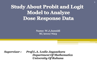


![• Likelihood Contribution
7
For single observation
When yi=1,p.d.f is Ф 𝑥𝑖 𝛽 and when yi=0 ,1 − Ф(𝑥𝑖 𝛽)
Likelihood is [∅(𝑥𝑖 𝛽)] 𝑦 𝑖 [1 − ∅(𝑥𝑖 𝛽)]1−𝑦 𝑖
For n observation
L β = [∅(xiβ)]yi [1 − ∅(xiβ)]1−yi
n
i=1
Log-likelihood function is
ln L β = yi∅(xiβ + 1 − yi
n
i=1 (1 − ∅(xiβ))]
∂lnL (β)
∂β
=
yi−∅(xiβ)
∅(xiβ)(1−∅(xiβ)
n
i=1 ∅(xiβ)xi
′
And
𝜕2
𝑙𝑛𝐿(𝛽)
𝜕𝛽𝜕𝛽′
= −
∅(𝑥𝑖 𝛽)2
∅(xiβ)(1 − ∅(xiβ)
𝑥𝑖
′
𝑥𝑖
𝑛
𝑖=1](https://image.slidesharecdn.com/probitandlogitmodel-150203022231-conversion-gate01/85/Probit-and-logit-model-7-320.jpg)


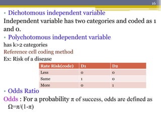
![• Likelihood function
13
Consider a sample of n independent observations of the pair (xi,yi) i=1,2….n
Pr y = 1|x = π x and Pr y = 0 x = 1 − π(x)
For the pair (xi,yi), likelihood function is π(xi)yi 1 − π(xi) 1−yi
Assume that observations are independent,
Likelihood function of n observation is L(β) = [π(xi)]yin
i=1 [1 − π(xi)]1−yi
lnL β = yilnπ xi + (1 − yi)ln(1 − π(xi))
n
i=1
To find the value of β that maximizes the lnL(β), differentiate lnL(β) w.r.t β0
and β1 and set the resulting expressions equal to zero.
yi − π xi = 0 and xi yi − π xi = 0](https://image.slidesharecdn.com/probitandlogitmodel-150203022231-conversion-gate01/85/Probit-and-logit-model-13-320.jpg)

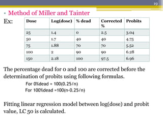
![• Score test
Based on the slope and expected curvature of the log-
likelihood function L(β) at the null value β0.
• Confidence interval
100(1-α)% C.I for the intercept and slope
• Multiple logistic model
15
u β = ∂L(β)/ ∂β|β0
= u β0
−E[∂2
L(β)/ ∂β2
|β0
] = τ β0
test st:u(β0)/[τ(β0)]1/2
~N(0,1)
β0 ± z1−α/2SE β0 and β1 ± z1−α/2SE β1
𝑔 𝑥 = 𝑙𝑛
𝜋(𝑥)
1 − 𝜋(𝑥)
= 𝛽0 + 𝛽1 𝑥1 + ⋯ + 𝛽𝑝 𝑥 𝑝](https://image.slidesharecdn.com/probitandlogitmodel-150203022231-conversion-gate01/85/Probit-and-logit-model-15-320.jpg)
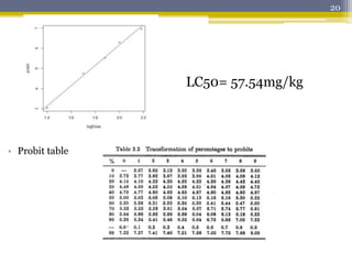
![Independent variable X
Outcome variable(y) X=1 X=0
Y=1
Y=0
Total 1 1
17
π 1 =
eβ0+β1
1 + eβ0+β1 𝜋 0 =
𝑒 𝛽0
1 + 𝑒 𝛽0
1 − 𝜋 1 =
1
𝑒 𝛽0+𝛽1
1 − 𝜋 0 =
1
1 + 𝑒 𝛽0
OR =
π(1)/[1 − π(1)]
π(0)/[1 − π(0)]
= eβ1
95% CI of ln OR = ln(OR) ± 1.96SE[ln OR ]
95% CI of OR = eln(OR )±1.96SE [ln OR ]
• Relative risk
Ratio of the two outcome probabilities
RR=π(1)/π(0)](https://image.slidesharecdn.com/probitandlogitmodel-150203022231-conversion-gate01/85/Probit-and-logit-model-17-320.jpg)


![Bibliography
[1]Razzaghi:Journal of Modern Applied Statistical Methods,Bloomsburg
University,May 2013, Vol. 12, No. 1, 164-169.
[2] Weng KeeWong,Peter A. Lachenbruch:Tutorial in Biostatistic and
Designing
studies for dose response,VOL.15,343-359(1996).
[3] Susan Ma:LC50 Sediment Testing of the Insecticide Fipronil with the Non-
Target
Organism,May 8 2006.
[4] Muhammad Akram Randhawa: http://www.ayubmed.edu.pk/JAMC/
PAST/21-3/ Randhawa,College of Medicine, University of Dammam:
2009;21(3).
[5] K. Bondari:Paper ST01,University of Georgia, Tifton,GA 31793-0748.
32](https://image.slidesharecdn.com/probitandlogitmodel-150203022231-conversion-gate01/85/Probit-and-logit-model-32-320.jpg)
![[6] Park, Hun Myoung:Regression models for binary dependent variables using
Stata, SAS, R, LIMDEP, and SPSS,Indiana University(2009).
[7] Probit Analysis By: Kim Vincent
[8] Mark Tranmer,Mark Elliot:Binary Logistic Regression
[9] DavidW. Hosmer,JR.,Stanley Lemeshow,Rodney X. Sturdivant:Applied Lo-
gistic Regression,Third Edition,ISBN 978-0-470-58247-3.
[10] Scott A. Czepiel:Maximum Likelihood Estimation of Logistic Regression Mod-
els,Theory and Implementation.
[11] Park, Hyeoun-Ae:An Introduction to Logistic Regression,Seoul National Uni-
versity,Korea,J Korean Acad Nurs Vol.43 No.2,April 2013.
[12] Finney, D. J., Ed. (1952). Probit Analysis,Cambridge, England, Cambridge
University Press.
33](https://image.slidesharecdn.com/probitandlogitmodel-150203022231-conversion-gate01/85/Probit-and-logit-model-33-320.jpg)


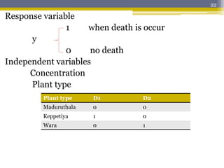
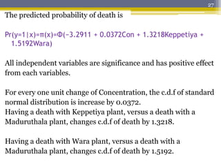
The document discusses the analysis of dose-response data using probit and logit models in the context of toxicology, particularly focusing on the effects of various botanical extracts on root knot nematodes. It highlights the calculation of LC50 values, the significance of coefficients in logistic models, and the predictive effects of concentration and plant type on mortality rates. Ultimately, it concludes that the wara plant extract is the most effective botanical for controlling the nematode population.


![Monitoring & evaluation presentation[1]](https://cdn.slidesharecdn.com/ss_thumbnails/monitoringevaluationpresentation1-110509033357-phpapp02-thumbnail.jpg?width=640&height=640&fit=bounds)


![[DSC Europe 25] Slobodan Dolinic - Smart and Intelligent Green Region.pptx](https://cdn.slidesharecdn.com/ss_thumbnails/0bribinjsp6ghwtvsvor-2-sigre-slobodan-dolinic-260115093812-c9c10e90-thumbnail.jpg?width=640&height=640&fit=bounds)


