panel data analysis with implications and importance
1.
Panel Data Econometrics
DongLi
Kansas State University
Fall 2009
Dong Li (Kansas State University) Panel Data Econometrics Fall 2009 1 / 115
2.
1 Introduction
Preliminary Definitionsand Some Examples
Some Characteristic Features
2
3
4
Benefits and Limitations of Panel Data
The One-Way Linear Models
Introduction
The Fixed Effects Model
The Random Effects Model
Feasible Generalized Least Square Method
(FGLS) Maximum Likelihood Estimation Method
(MLE)
One-Way Models in Stata
Motivations for Panel Methods
Hypothesis Testing in One-Way Models
Test for Poolability
Tests for Individual Effects
Test for Fixed Effects Test
for Random Effects
The Hausman Test: The
Random Effects vs.
Dong Li (Kansas State University) Panel Data Econometrics Fall 2009 1 / 115
3.
The Fixed EffectsModel
The Random Effects Model
5
6
7
8
9
10
11
Treatment Effects and Difference-in-Differences
Treatment Effects
Difference-in-Differences
Heteroskedasticity and Serial Correlation
Heteroskedasticity
Serial Correlation
Implementations in LIMDEP/Stata/EViews
Simultaneous Equations with Error Components
Endogenous Regressors
Endogenous Individual Effects
Linear Dynamic Models
The Arellano and Bond Study
Nonlinear Panel Data Models/Limited Dependent Variable Models
Spatial Models
Field Experiments
Dong Li (Kansas State University) Panel Data Econometrics Fall 2009 2 / 115
4.
Panel Data: Individualscan be true individuals or households, firms,
states, countries, etc.
The sample size N × T . N and T may be very different (large N and
small T , or small N and largeT ) - this is important in choosing
models.
Dong Li (Kansas State University) Panel Data Econometrics Fall 2009 2 / 115
5.
Panel data -Cross Sectional Time Series.
Repeated measurements (biometrics): growth of rat i at time t.
Longitudinal Data (demography, sociology).
It has many communalities with spatio-temporal data, multilevel
analysis.
Dong Li (Kansas State University) Panel Data Econometrics Fall 2009 3 / 115
6.
Some of theAvailable Micro Data Sets
U.S. data sets:
The Panel Study of Income Dynamics (PSID): collected by University
of Michigan www.isr.umich.edu/src/psid/index.html
the National Longitudinal Surveys of Labor Market Experience (NLS)
from the Center for Human Resource Research at Ohio State
University and the Census Bureau. www.bls.gov/nlshome.htm
Medical Expenditure Panel Survey www.meps.ahrq.gov/mepsweb
Longitudinal retirement history supply
Social Security Administration’s Continuous Work History Sample
Labor Department’s continuous wage and benefit history
Labor Department’s continuous longitudinal manpower survey
Negative income tax experiments
Current Population Survey
Dong Li (Kansas State University) Panel Data Econometrics Fall 2009 4 / 115
7.
International:
The German Social-EconomicPanel (GSOEP)
The Belgian Socioeconomic Panel
The Canadian Survey of Labor Income Dynamics (SLID)
The French Household Panel
The Hungarian Household Panel
The British Household Panel Survey
The Japanese Panel Survey on
Consumers (JPSC)
Dong Li (Kansas State University) Panel Data Econometrics Fall 2009 5 / 115
8.
Sample size: typicallyN is large and T is small. But it is not always the
case.
Sampling: often individuals are selected randomly, at least at the
beginning of the sample, but time is not.
Non-independent data:
Among data to the same individual: because of unobservable
characteristics of each individual.
Among individuals: because of unobservable characteristics common
to several individuals.
between time period: because of dynamic behavior.
Dong Li (Kansas State University) Panel Data Econometrics Fall 2009 6 / 115
9.
Benefits:
1 Controlling forindividual heterogeneity.
Panel data gives more informative data, more variability, less
collinearity among the variables, and more degrees of freedom.
Panel data is better able to study the dynamics of adjustment.
Panel data is better able to identify and measure effects that are simply
not detectable in pure cross-sections or pure time-series data. Such as
study of union membership.
Panel data models allow us to construct and test more complicated
behavioral models than purely cross-section or time-series data. For
example, technical efficiency is better studied and modeled with
panels.
Panel data is usually gathered on micro units, like individuals, firms
and households. Many variables can be more accurately measured at
the micro level, and biases resulting from aggregation over firms or
individuals are eliminated, see Blundell (1988) and Klevmarken (1989).
2
3
4
5
6
Dong Li (Kansas State University) Panel Data Econometrics Fall 2009 7 / 115
10.
Limitations:
1 Design anddata collection problems. These include problems of
coverage (incomplete account of the population of interest),
nonresponse (due to lack of cooperation of the respondent or because
of interviewer error), recall (respondent not remembering correctly),
frequency of interviewing, interview spacing, reference period, the use
of bounding and time-in-sample bias, . . . .
Distortions of measurement errors. Measurement errors may arise
because of faulty responses due to unclear questions, memory errors,
deliberate distortion of responses (e.g. prestige bias), inappropriate
informants, misrecording of responses and interviewer effects.
Selectivity problems.
2
3
1 Self-selectivity.
Non-response.
Attrition.
2
3
4
Dong Li (Kansas State University) Panel Data Econometrics Fall 2009 8 / 115
Short Time Series Dimension. Asymptotics and limited dependent
variable models.
11.
A panel dataregression has a double subscript on its variables:
it
yit = α + X 𝐹
ß + uit , i = 1,..., N; t = 1,..., T . (1)
i denotes individuals, households, firms, countries, etc., the
cross-section dimension.
t denotes time, the time-series dimension.
α is a scalar, ß is K × 1 and Xit is the it-th observation on K explanatory
variables.
Dong Li (Kansas State University) Panel Data Econometrics Fall 2009 9 / 115
12.
Most of thepanel data applications utilize a one-way model
uit = µi + νit
(2)
where µi denotes the unobservable individual specific effect and νit
denotes the remainder disturbance.
For example, in an earnings equation in labor economics, µi may
include the individual’s (time-invariant) unobserved ability.
A production function utilizing data on firms across time, µi may
capture the unobservable entrepreneurial or managerial skills of the
firm’s executives.
The remainder disturbance νit varies with individuals and time and
can be thought of as the usual disturbance in the regression.
Dong Li (Kansas State University) Panel Data Econometrics Fall 2009 10 / 115
13.
It is calleda balanced panel if every individual has the same time span
t = 1, ..., T .
It is called an unbalanced panel if not so (then we have total number
of observations
, N
i=1 Ti).
We are going to assume we have balanced panel throughout the
semester unless otherwise noted.
The unbalanced panel estimation can be obtained similar to the
balanced one. Most statistical software can take care of it
“automatically.”
Dong Li (Kansas State University) Panel Data Econometrics Fall 2009 11 / 115
14.
In vector form(1) can be written as
(3)
y = αιN T + Xß + u = Z δ + u
where y is NT × 1, X is NT × K , Z = [ιNT , X ], δ𝐹 = (α𝐹, ß 𝐹), and ιN T is
a vector of ones of dimension NT = N × T .
(2) can be written in matrix form as
u = Zµ µ + ν
where u𝐹 = (u1 1 ,..., u1 T , u2 1 ,..., u2 T , . . . , uN 1 ,..., uN T ) with
the
(4)
observations stacked such that the slower index is over individuals and
the faster index is over time.
Zµ = IN ⊗ ιT where IN is an identity matrix of dimension N, ιT is a
vector of ones of dimension T , and ⊗ denotes Kronecker product.
Zµ is a selector matrix of ones and zeros, or simply the matrix of
individual dummies that one may include in the regression to estimate
the µi’s if they are assumed to be fixed parameters. µ𝐹 = (µ1 ,..., µN )
and ν 𝐹 = (ν1 1 ,..., ν1T , . . . , νN 1 ,..., νN T ).
Dong Li (Kansas State University) Panel Data Econometrics Fall 2009 12 / 115
15.
Matrices P andQ
Z𝐹 Zµ = (IN ⊗ ι𝐹
)(IN ⊗ ιT ) = IN ⊗ T = TIN .
µ T
The projection matrix,
µ µ T N T
P = Zµ(Z𝐹 Zµ)−1Z𝐹 = (IN ⊗ ιT ) 1
I−1
(IN ⊗ ι𝐹
) = IN ⊗ J¯T , where J¯T =
JT /T
(average matrix) and JT is a matrix of ones of dimension T × T .
P is a matrix which averages the observation across time for each
individual, and Q = INT − P = IN ⊗ (IT − J¯T ) is a matrix which
obtains the deviations from individual means.
i·
For example, Pu has a typical element u¯ =
, T
t=1 ui t /T repeated T
times for each individual and Qu has a typical element (uit − u¯
i·).
Dong Li (Kansas State University) Panel Data Econometrics Fall 2009 13 / 115
16.
Matrices P andQ
Properties of P and Q:
P and Q are symmetric idempotent matrices, i.e., P𝐹 = P and P2 = P.
This means that the rank(P) = tr(P) = N and rank(Q) = tr(Q) =
N(T − 1). This uses the result that rank of an idempotent matrix is
equal to its trace, see Graybill (1961, Theorem 1.63).
P and Q are orthogonal, i.e., PQ = 0.
They sum to the identity matrix P + Q = INT .
Any two of these properties imply the third, see Graybill (1961, Theorem
1.68).
Dong Li (Kansas State University) Panel Data Econometrics Fall 2009 14 / 115
17.
The µi’s areassumed to be fixed parameters to be estimated.
The remainder disturbances are stochastic with νit ∼ IID(0, σ 2 ).
ν
The Xit ’s are assumed independent of the νit ’s for all i and t. (We will
relax this assumption later.)
The fixed effects model is an appropriate specification if we are
focusing on a specific set of N firms and our inference is restricted to
the behavior of these sets of firms. Alternatively, it could be a set of N
OECD countries, or N American States. Inference in this case is
conditional on the particular N firms, countries, or states that are
observed.
One can substitute the disturbances given by (4) into (3) to get
y = αιN T + Xß + Zµ µ + ν = Z δ + Zµ µ + ν . (5)
Dong Li (Kansas State University) Panel Data Econometrics Fall 2009 15 / 115
18.
Methods to estimatethe FE model
Method 1: Brutal force OLS
Brutal force OLS on (5) to get estimates of α, ß and µ: Note that Z is
NT × (K + 1) and Zµ , the matrix of individual dummies is NT × N. If N is
large, (5) will include too many individual dummies, and the matrix to be
inverted by OLS is large and of dimension (N + K ). It is not feasible in most
statistical software when N is large.
Dong Li (Kansas State University) Panel Data Econometrics Fall 2009 16 / 115
19.
Methods to estimatethe FE model
Method 2: Demeaning
Since α and ß are the parameters of interest, one can obtain the estimates
from (5) by pre-multiplying the model by Q and performing OLS on the
resulting transformed model:
Qy = QXß + Qν
(6)
This uses the fact that QZµ = QιN T = 0, since PZµ = Zµ . In other words, the Q
matrix wipes out the individual effects. This is a regression of y˜ = Qy with
typical element (yit − y¯i·) on X˜ = QX with typical element (Xit,k − X¯i·,k) for
the k-th regressor, k = 1, 2,..., K . This involves the inversion of a (K × K )
matrix rather than (N + K ) × (N + K ) as in (5). The resulting OLS estimator is
ߘ = (X 𝐹
QX )−1
X 𝐹
Qy
ν ν
with Var(ߘ) = σ 2 (X 𝐹QX )−1 = σ 2 (X˜ 𝐹X˜ )−1. Notice the variance-
covariance
matrix.
Dong Li (Kansas State University) Panel Data Econometrics Fall 2009 17 / 115
20.
Methods to estimatethe FE model
Method 3: Generalized Least Squares
ν
GLS on (5): Var(Qν ) = σ 2 Q. So the GLS estimator
߈ = ((QX )𝐹
(σ2
Q)−1
(QX ))−1
(QX )𝐹
(σ2
Q)−1
(Qy) = (X 𝐹
QX )−1
X 𝐹
Qy
ν ν
with Var(ߘ) = σ 2 (X 𝐹QX )−1 = σ 2 (X˜ 𝐹X˜ )−1.
ν ν
Dong Li (Kansas State University) Panel Data Econometrics Fall 2009 18 / 115
21.
Methods to estimatethe FE model
While the theory in the above estimation discussions is simple, it may not
be practical to implement these three methods.
When NT is large (for example, N = 1000 and T = 10: it means that Q is a
10000 by 10000 matrix. in GAUSS it takes 8 × 108 bytes or roughly 763MB.
Imagine that you need more space to operate on it) pre-multiplying the
model by Q in the above methods 2 and 3 is infeasible in most statistical
software.
Dong Li (Kansas State University) Panel Data Econometrics Fall 2009 19 / 115
22.
Methods to estimatethe FE model
Method 4: Within(demean) transformation in scalar
Consider the within transformation without matrix notation for the simple
regression
(8)
yit = α + ßxi t + µi + νit .
Averaging over time for each individual gives the between regression
y¯i· = α + ß x¯i· + µi + ν¯i·
and the difference between the above two regressions gives the within
regression
yit − y¯i· = ß (xit − x¯i·) + (νit − ν¯i·)
also averaging across all observations gives
y¯.
. = α + ß x¯..+ ν¯..
(9)
(10)
(11)
,
i
where we utilized the restriction that µ = 0. This is an arbitrary
restriction on the dummy variable coefficients to avoid the dummy variable
trap, or perfect multicollinearity.
Dong Li (Kansas State University) Panel Data Econometrics Fall 2009 20 / 115
23.
ߘ is obtainedfrom regression (10), α˜ = y¯.
. − ߘx¯.. can be recovered from
the last equation and µ˜ i = y¯i· − α˜ − ߘx¯i· from (9).
Dong Li (Kansas State University) Panel Data Econometrics Fall 2009 21 / 115
24.
Possible drawbacks forthe FE model
1 The fixed effects (FE) least squares, also known as least squares
dummy variables (LSDV) suffers from a large loss of degrees of
freedom.
We are estimating (N − 1) extra parameters, and too many dummies
may aggravate the problem of multicollinearity among the regressors.
In addition, the FE estimator cannot estimate the effect of any time
invariant variable like sex, race, religion, schooling, or union
participation. These time invariant variables are wiped out by the Q
transformation, the deviation-from-mean transformation.
If the FE model is the true model, LSDV is BLUE as long as ν is a
standard classical disturbance with mean 0 and variance covariance
2
3
4
matrix σ 2 INT . Note that as T → ∞, the FE estimator is consistent.
ν
However, if T is fixed and N → ∞ as typical in short labor panels, then
only the FE estimator of ß is consistent, the FE estimators of the
individual effects (α + µi) are not consistent since the number of these
parameters increase as N increases.
Dong Li (Kansas State University) Panel Data Econometrics Fall 2009 22 / 115
25.
A few comments
1Testing for fixed effects. One could test the joint significance of these
dummies, i.e., H0: µ1 = ... = µN − 1 = 0, by performing an F test. This is a
simple F test with the RRSS being that of OLS on the pooled model
and the URSS being that of the LSDV regression.
F =
(RRSS − URSS)/(N −
1)
URSS/(NT − N − K )
H0
∼ FN−1,N(T −1)−K (12)
This test is available after FE regression in Stata.
Computational Warning. One computational caution for those using
the within regression given by (10). The s2 of this regression as
obtained from a typical regression package divides the residual sums
of squares by NT − K since the intercept and the dummies are not
included. The proper s2, say s∗2 from the LSDV regression would divide
the same residual sums of squares by N(T − 1) − K . Therefore, one has
to adjust the variances obtained from the within regression (10) by
multiplying the variance-covariance matrix by (s∗2/s2) or simply by
multiplying by [NT − K ]/[N(T − 1) − K ].
2
Dong Li (Kansas State University) Panel Data Econometrics Fall 2009 23 / 115
26.
Method 5: FirstDifference
First difference the model (1) to get
∆yit = ∆X 𝐹
ß + ∆ui t = ∆X 𝐹
ß + ∆νit , i = 1,..., N; t = 2,..., T .
(13)
it it
where ∆yit = yit − yi,t−1. The original model can be fixed effects or random
effects. But FD is mostly used in the fixed effects model. It offers another
method to remove the individual effects.
Dong Li (Kansas State University) Panel Data Econometrics Fall 2009 24 / 115
27.
Some potential drawbackswith first difference method
1 Any time-invariant regressor would result in a column of 0s and we
cannot estimate its effect.
Some time variant variables may result in a constant term. For
example, variable age in yearly data would generate ∆age = 1.
If the temporal variation of xit is small, i.e., ∆xit is small, we get to
estimate the coefficients with low precision in the differenced model.
2
3
We will discuss the first difference model with more details in the dynamic
models.
Dong Li (Kansas State University) Panel Data Econometrics Fall 2009 25 / 115
28.
Assumptions
1
µ
µi ∼ IID(0,σ 2 );
2 νit ∼ IID(0, σ 2 );
ν
µi’s are independent of the νit ’s;
In addition, the Xit ’s are independent of the µi’s and νit ’s for all i and t.
This is the cost of random effects model compared to the fixed effects
model.
3
4
Dong Li (Kansas State University) Panel Data Econometrics Fall 2009 26 / 115
29.
The random effectsmodel is an appropriate specification if we are drawing
N individuals randomly from a large population. This is usually the case for
household panel studies. Care is taken in the design of the panel to make it
‘representative’ of the population we are trying to make inference about. In
this case, N is usually large and a fixed effects model would lead to an
enormous loss of degrees of freedom. The individual effect is characterized
as random and inference pertains to the population from which this
sample was randomly drawn.
Dong Li (Kansas State University) Panel Data Econometrics Fall 2009 27 / 115
30.
Estimation
From (4), onecan compute the variance-covariance matrix
µ
Ω = E(uu𝐹
) = ZµE(µµ𝐹
)Z𝐹
+ E(νν 𝐹
) (14)
(15)
= σ 2
(IN ⊗ JT ) + σ 2
(IN ⊗ IT )
µ ν
This implies a homoskedastic variance Var(uit ) = σ 2 + σ 2 for all i and t, and
µ ν
an equi-correlated block-diagonal covariance matrix
which exhibits serial
correlation over time only between the disturbances of
the same individual.
2
µ
2
ν
σ + σ , for i = j, t = s;
for i = j, t /=
s; for i /= j.
µ
Cov(uit , ujs) =
σ 2 ,
0,
Dong Li (Kansas State University) Panel Data Econometrics Fall 2009 28 / 115
31.
The variance-covariance matrixE(uu𝐹) is given by
Dong Li (Kansas State University) Panel Data Econometrics Fall 2009 29 / 115
Ω =
µ
σ 2 2
u σ ...
σ
2
µ
σ µ
2 σ 2
u ..
. .
.
.
.
. .
.. .. σ 2
µ
2 2
σ µ ... σ µ σ
2
u
0 0
0
0
(. . .) 0
0 (. .
.)
where σ 2 = Var(uit ) = σ 2 + σ 2 .
u
µ
ν
32.
The correlation coefficientbetween uit and ujs is
Corr(uit , ujs) =
1, for i = j, t = s;
for i = j, t /=
s; otherwise.
σ 2
σ 2 +σ2
µ
,
µ
ν
0,
(16)
To obtain the GLS estimator of the regression coefficients, we need
Ω−1.
This is a huge matrix for typical panels and is of dimension (NT × NT ).
Impractical to invert the matrix using brutal force.
Results in Wansbeek and Kapteyn (1982b,1983) provide the derivations
of Ω−1 and Ω−1/2.
Dong Li (Kansas State University) Panel Data Econometrics Fall 2009 30 / 115
33.
Define ET =IT − J¯T . Replace JT by T J¯T , and IT by (ET + J¯T ).
Then
Ω = T σ 2
(IN ⊗ J¯T ) + σ 2
(IN ⊗ ET ) + σ 2
(IN ⊗ J¯T )
µ ν
ν
= (Tσ2
+ σ 2
)(IN ⊗ J¯T ) + σ 2
(IN ⊗ ET )
µ ν
ν
= σ2
P + σ 2
Q
1
ν
(17)
where σ 2
= T σ 2 + σ 2 .
1
µ
ν
1
This is the spectral decomposition representation of Ω, with σ 2
being
the first unique characteristic root of Ω of multiplicity N and σ 2 is the
ν
second unique characteristic root of Ω of multiplicity N(T − 1).
It is easy to verify, using the properties of P and Q, that
1
σ 2 σ 2
ν
Ω−1
=
1
P +
1
Q
(18)
and
Ω−1/2
=
1
P +
1
Q.
σ1
σ ν
(19)
Dong Li (Kansas State University) Panel Data Econometrics Fall 2009 31 / 115
34.
Now we canobtain GLS estimator without actually inverting NT × NT
matrix Ω
δ = (Z𝐹
Ω−1
Z)−1
Z𝐹
Ω−1
y.
(20)
− 1
GLS is the BLUE.
Fuller and Battese (1973, 1974) suggested pre-multiplying the
regression equation given in (3) by σ ν Ω 2 = Q + (σν /σ1 )P and
performing OLS on the resulting transformed regression. This was
particularly helpful in the old days when OLS was a big deal in
computation.
∗ − 1
2
ν it i·
In this case, y = σ Ω y has a typical element y − θ y¯
where
θ = 1 − (σν /σ1 ). This transformed regression only requires inversion
of a matrix of dimension (K+1) and can be easily implemented using
any regression package. Notice that you have to transform every
variable, including the intercept. Also when you run the transformed
regression, make sure no constant is included.
Dong Li (Kansas State University) Panel Data Econometrics Fall 2009 32 / 115
35.
But the abovemethod is not feasible yet since we do not know σ 1 or
σ ν .
The Best Quadratic Unbiased (BQU) estimators of the variance
components arise naturally from the spectral decomposition of Ω:
2 u𝐹Pu
σˆ 1 =
tr(P)
where trP = N. (21)
2 u𝐹Qu
σˆ ν =
tr(Q)
where trQ = N(T − 1). (22)
Dong Li (Kansas State University) Panel Data Econometrics Fall 2009 33 / 115
36.
We can showthat the above estimators are unbiased.
E(u𝐹
Qu) = E(tr(u𝐹
Qu)) = E(tr(uu𝐹
Q)) = tr(E(uu𝐹
Q)) = tr(E(uu𝐹
)Q)
= tr(ΩQ) = tr[(σ2
P + σ 2
Q)Q] = tr(σ2
Q) = σ 2
trQ
1
ν
ν
ν
So
ν
E(σˆ 2
) = E
�
�
u Qu
= ν
σ 2 tr(Q)
tr(Q) tr(Q)
Dong Li (Kansas State University) Panel Data Econometrics Fall 2009 34 / 115
ν
= σ 2
.
Similar results can be obtained for σˆ 2
.
1
The true disturbances u are not known and therefore (21) and (22) are not
feasible. How to estimate u (uˆ) to make the GLS feasible (FGLS)?
37.
Ways to estimatethe error components:
1 Wallace and Hussain (1969) suggest substituting OLS residuals
uˆOLS instead of the true u’s, because the OLS estimates are still
unbiased and consistent, though no longer efficient.
Amemiya (1971) shows that the Wallace and Hussain estimators of the
variance components have a different asymptotic distribution from
that knowing the true disturbances. He suggests using the LSDV
residuals instead of the OLS residuals.
Swamy and Arora (1972) suggest running two regressions to get
estimates of the variance components from the corresponding mean
square errors of these regressions. The first regression is the Within
regression which yields
2
3
σ
^
2
ν
𝐹 𝐹 𝐹
−1 𝐹
= [y Qy − y QX (X QX ) X Qy]/[N(T − 1) − K ]. The
second
regression is the Between regression which yields
σ
^
2
𝐹
1
𝐹
𝐹
= [y Py − y PZ(Z PZ −1
𝐹
) Z Py]/(N − K −
1
).
4 2
, N
µ i=1
¯ 2
Nerlove (1971) suggests σˆ = (µˆ − µˆ) /(N
− 1
i i
) where µˆ are the
ν
dummy coefficients estimates from the LSDV regression. σˆ 2 is
estimated from the within residual sums of squares divided by NT
without correction for degrees of freedom.
Dong Li (Kansas State University) Panel Data Econometrics Fall 2009 35 / 115
38.
Some further discussionson the Swamy-Arora method: Note that stacking
the two transformed regressions, the between and the within regression,
yields
Qy
Py
‚ Œ ‚
=
QZ
PZ
Œ ‚
δ +
Qu
Pu
Œ
(23)
and the transformed error has mean 0 and variance-covariance matrix
given by
2
ν
σ Q 0
1
0 σ2
P
‚ Œ
.
OLS on this system of 2NT observations yields OLS on the pooled
model (3). Also, GLS on this system yields GLS on (3). (This means the
two transformations have not lost any information here.)
One can show that the GLS random effects estimator is a weighted
average of the within estimator and the between estimator:
߈GLS = W ߈Between + (I − W )߈Within.
Dong Li (Kansas State University) Panel Data Econometrics Fall 2009 36 / 115
39.
A significant “drawback"of random effects model is that it is assumed that
the individual effects are not correlated with xit , which is questionable in
many applications.
Dong Li (Kansas State University) Panel Data Econometrics Fall 2009 37 / 115
40.
1 ν
Note thatΩ = E(uu𝐹) = σ2
P + σ 2 Q. So the loglikelihood function is
log L = −
NT
ln(2𝑢) −
1
ln|Ω| −
1
u𝐹
Ω−1
u
2 2
2
Dong Li (Kansas State University) Panel Data Econometrics Fall 2009 38 / 115
NT 1
2 2 1 ν
= − ln(2𝑢) − ln(σ ) (σ )
2 N 2 N(T
−1) 2
− u �
�
‚
1 1
σ 2
1
1
σ 2
ν
P + Q u
Œ
(by noting that |A| =
ℎ1 ℎ2 ...ℎn )
41.
Specify the iand t variables: tsset id year or xtset id year
One benefit is that afterwards you can use the lag operator. In a panel
setup, lag will be within each individual.
Sample Stata program.
Dong Li (Kansas State University) Panel Data Econometrics Fall 2009 39 / 115
42.
If the (unobserved)individual effects µi’s are random, the error terms
uit are autocorrelated (but homoscedastic). The OLS estimators are
still unbiased, but not efficient. The OLS standard errors are
misleading.
If the (unobserved) individual effects µi’s are fixed and we run OLS
without µ in the regression, it causes the omitted variable problem
(omission of relevant variables). The OLS estimators are biased.
If the true model is y = Xß + Zγ + u but we estimate y = Xß + u instead
(ߘ = (X 𝐹X )−1X 𝐹y), we have
ߘ = (X 𝐹
X )−1
X 𝐹
(Xß + Z γ + u)
= ß + (X 𝐹
X )−1
X 𝐹
Zγ + (X 𝐹
X )−1
X
𝐹
u
So
E(ߘ) = ß + E[(X 𝐹
X )−1
X 𝐹
Z]γ + 0
(24)
The above expectation is not ß unless the second term is zero.
Dong Li (Kansas State University) Panel Data Econometrics Fall 2009 40 / 115
43.
Appendix 2A: Traceof a (Square) Matrix
Dong Li (Kansas State University) Panel Data Econometrics Fall 2009 41 / 115
The trace of a square n × n matrix A, denoted tr(A), is the sum of its diagonal
, n
i=1 aii.
elements: tr(A) =
We have
tr(A + B)
tr(kA)
trA𝐹
tr(AB)
= trA + trB
= k trA
= trA
= tr(BA)
(25)
(26)
(27)
(28)
44.
Appendix 2B: TheKronecker Product
Let A be an m × n matrix and B a p × q matrix. The mp × nq matrix defined
by
Dong Li (Kansas State University) Panel Data Econometrics Fall 2009 42 / 115
11 1n
a B ... a B
. .
. .
a B ... a B
m1 mn
is called the Kronecker product of A and B and written A ⊗ B.
Some properties of the Kronecker product:
A ⊗ B ⊗ C = (A ⊗ B) ⊗ C = A ⊗ (B ⊗ C)
(A + B) ⊗ (C + D) = A ⊗ C + A ⊗ D + B ⊗ C + B ⊗ D if A + B and C + D
exist
(A ⊗ B)(C ⊗ D) = AC ⊗ BD if AC and BD exist
(A ⊗ B)𝐹 = A𝐹
⊗ B𝐹
(A ⊗ B)−1
= A−1
⊗ B−1
if A and B are non-singular.
45.
Appendix 2C: Eigenvectorand Eigenvalue
A scalar (real number) ℎ is said to be an eigenvalue of an n × n matrix A if
there exists an n × 1 non-null vector x such that Ax = x
ℎ . x is called the
eigenvector associated with ℎ. Eigenvalues are solutions to |A − I
ℎ | = 0.
Two important properties:
trA = ℎ1 + ℎ2 + ... + ℎn
and
|A| = ℎ1 ℎ2 ...ℎn .
Dong Li (Kansas State University) Panel Data Econometrics Fall 2009 43 / 115
46.
Appendix 2D: MatrixCalculus
Suppose that we have the vectors a, x, and the matrix B defined as
a1
x1
a = a
a3
2
x = x
x3
2
b31 b32 b33
b11 b12 b13
B = b b b
21 22
23
�
�
Then L = a x =
, 3
i=1 aixi is said to be a linear form in x and
�
�
Q = x Bx =
, ,
3 3
i=1 j=1 bij xi xj is said to be a quadratic form in x. If the
dimension of the vectors and matrix is more than 3, the following rules still
apply.
Note that ∂ L/∂ xi = ai. We shall denote the vector of partial derivatives
∂ L
∂ x1
∂ L
∂ x
∂ L
∂ x3
2
by ∂ L/∂ x. Thus we have ∂ L/∂ x = a. We also have
∂ Q
∂ x
= Bx + B𝐹
x
= 2Bx if B is symmetric
Dong Li (Kansas State University) Panel Data Econometrics Fall 2009 44 / 115
47.
Appendix 2E: PartitionedRegression Consider a partition regression
y = Zß + W γ + e = Xδ + e where all are matrices. To estimate ß without
estimating γ.
Dong Li (Kansas State University) Panel Data Econometrics Fall 2009 45 / 115
Recall that the normal equation for OLS is X 𝐹X δˆ = X 𝐹y, which is equivalent
to Z�
�
W
𝐹
Š
ˆ
W δ =
�
�
Z y
W
𝐹y
‚ Œ
(29)
and ‚
�
�
‚ Œ
€
Z
Z Z Z𝐹W
W 𝐹Z
W 𝐹W
ˆ
ß
γ
ˆ
Œ‚ Œ ‚
=
�
�
Z y
W
𝐹y
Œ
(30)
and
Z𝐹
Z߈ + Z𝐹
W γˆ = Z𝐹
y
W 𝐹
Z߈ + W 𝐹
W γˆ = W
𝐹
y
(31)
(32)
48.
From (32) onecan find γˆ = (W 𝐹W )−1W 𝐹(y − Z߈). Plug this equation into
(31) one can obtain
Z𝐹
Z߈ + Z𝐹
W (W 𝐹
W )−1
W 𝐹
(y − Z߈) = Z𝐹
y
Z𝐹
Z߈ − Z𝐹
W (W 𝐹
W )−1
W 𝐹
Z߈ = Z𝐹
y − Z𝐹
W (W 𝐹
W )
−1
W 𝐹
y
Z𝐹
[I − W (W 𝐹
W )−1
W 𝐹
]Z߈ = Z𝐹
[I − W (W 𝐹
W )−1
W 𝐹
]y
(33)
(34)
(35)
Define PW = W (W 𝐹W )−1W 𝐹 and P¯ W = I − PW . PW is the projection
matrix and P¯ W is the residual projection. It is easy to verify that both PW
and P¯ W are symmetric and idempotent. The above equation becomes
(Z𝐹
P¯ W Z)߈ = Z𝐹
P¯ W y
߈ = (Z𝐹
P¯ W Z)−1
Z𝐹
P¯
W y
(36)
(37)
which is also the OLS estimator from the following regression
P¯ W y = P¯ W Zß + P¯ W e.
Dong Li (Kansas State University) Panel Data Econometrics Fall 2009 46 / 115
49.
Consider two regressions:
Regressy on Z and W to obtain ߈;
regress y on W and obtain the residuals; regress Z on W and obtain the
residuals; regress the first set of residuals on the second set of residuals
and obtain the coefficients ߘ.
The Frisch-Waugh-Lovell Theorem (FWL) states: ߈ and ߘ are identical; the
residuals from the partitioned regression are identical to the residuals from
the original regression.
Dong Li (Kansas State University) Panel Data Econometrics Fall 2009 46 / 115
50.
References
Harville, D.A., MatrixAlgebra from a Statistician’s Perspective, Springer,
1997
Magnus, J.R. and H. Neudecker, Matrix Differential Calculus with
Applications in Statistics and Econometrics, Wiley, 1988.
Berck, P. and K. Sydsaeter, Economists’s Mathematical Manual, Second
Ed, Springer-Verlag, 1993.
Dong Li (Kansas State University) Panel Data Econometrics Fall 2009 47 / 115
51.
The first questionwe want to ask is whether we can pool the different
individuals, firms, states, regions, countries together.
For the unrestricted model, we have a regression equation for each
region given by
yi = Zi δi + ui for i = 1, 2, ..., N
(38)
where y𝐹
= (yi1, ..., yiT ), Zi = (ιT , Xi) and Xi is T × K . δ𝐹
is 1 × (K + 1)
and
i i
ui is T × 1.
Note that δi is different for every i. This unrestricted model can be
written as
2
.
.
yN
=
y
1 1
0
.
.
0 0
y Z 0 . . . 0
Z2
. . .
...
. . .
ZN
2
. .
. .
δ N
δ 1
0 δ
+ u (39)
Dong Li (Kansas State University) Panel Data Econometrics Fall 2009 48 / 115
52.
We want totest the hypothesis H0 : δi = δ for all i, so that under H0 we
can write the restricted model as
y1
Z1
=
y
Z
2 2
. .
. .
y Z
N N
δ + u
(40)
Under assumption u ∼ N(0, σ2 IN T ) the test becomes a Chow test (F
test). You can get the Unrestricted RSS from the separate regressions in
(38) and add them up. You can obtain the Restricted RSS from (40).
If u ∼ N(0, σ2 Ω) the test becomes a Chow test (F test) for a GLS model.
Dong Li (Kansas State University) Panel Data Econometrics Fall 2009 49 / 115
53.
You want totest the null hypothesis H0 : µ1 = ... = µN − 1 = 0.
The unrestricted model is
it
yit = α + X 𝐹
ß + µi + νit , i = 1,..., N; t = 1,...,
T .
(41)
The restricted model is
it
yit = α + X 𝐹
ß + νit , i = 1,..., N; t = 1,...,
T .
(42)
The F test is
(RRSS − URSS)/(N −
1)URSS/(NT − N − K
)
H0
F = ∼ FN−1,N(T −1)−K (43)
Stata actually reports this F test after fixed effects estimation.
Dong Li (Kansas State University) Panel Data Econometrics Fall 2009 50 / 115
54.
Consider
it
yit = α+ X 𝐹
ß + µi + νit , i = 1,..., N; t = 1,..., T . (44)
where µi ∼ IID N(0, σ 2 ). We derived the loglikelihood function in
µ
Chapter 2. The Lagrange Multiplier (LM) test to test H0 : σ 2 = 0, also
µ
called the Breusch-Pagan test, can be constructed based on
the logl.
In Stata the command xttest0 after random effects estimation will
give the test result.
Honda (1985) modified the test to account for the fact that the
alternative is one-sided σ 2 > 0.
µ
Moulton and Randolph (1989) and Honda (1991) further standardize
the above test by subtracting its mean and then divided by its standard
deviation.
Dong Li (Kansas State University) Panel Data Econometrics Fall 2009 51 / 115
55.
Some comparisons betweenthe random effects model and the fixed effects
model:
The fixed effects model loses large degrees of freedom (N − 1).
The fixed effects model allows the individual effects to be correlated
with the regressors.
If you want to estimate time-invariant variables in the panel data
model, you have to use the random effects model.
If we want to make inference only this set of cross-sectional units then
we should treat µi’s as fixed. On the other hand, if we want to make
inference about the population from which the cross sectional data
came, we should treat µi as random. In most of the applied
econometric work, the latter is the case.
Dong Li (Kansas State University) Panel Data Econometrics Fall 2009 52 / 115
56.
The Hausman Test
TheHausman test is based on the following idea: If H0 is true, FE and RE
estimators are close to each other; otherwise they are very different from
each other.
Table: The Hausman Test
Under H0 H1
RE
FE
consistent and efficient
consistent but inefficient
inconsistent
consistent
H0: There is no correlation between µi’s and regressors.
H1: There may exist correlation between µi’s and regressors.
This same idea leads to the Hausman test for OLS vs. IV.
Dong Li (Kansas State University) Panel Data Econometrics Fall 2009 53 / 115
57.
A “mechanic” wayto decide the model choice between the fixed
effects and the random effects. Compare the difference between the
random effects estimates and the fixed effects estimates. If the
difference is significant, we go for the fixed effects. If not, go for the
random effects (because it is more efficient).
H0 : µi’s are uncorrelated with X 𝐹
versus H1 : µi’s are correlated with
it
X 𝐹
. The fixed effects model is unbiased and consistent under H0
and
it
H1. It is efficient under H1 but inefficient under H0. The random
effects model is biased and inconsistent under H1 but consistent and
efficient under H0.
Define qˆ = ߈FE − ߈RE . It turns out that Var(qˆ) = Var(߈FE ) −
Var(߈RE ) under H0:
Var(qˆ) = Var(߈FE − ߈RE )
= Var(߈FE ) + Var(߈RE ) − 2Cov(߈FE , ߈RE )
= Var(߈FE ) + Var(߈RE ) − 2(X 𝐹
Ω−1
X )−1
X 𝐹
Ω−1
E(uu𝐹
)QX
(X 𝐹
QX )−1
Dong Li (Kansas State University) Panel Data Econometrics Fall 2009 54 / 115
58.
The test statistic
m= qˆ𝐹
[Var(qˆ)]− 1
qˆ (45)
K
and under H0 it is asymptotically distributed as χ 2
, where K denotes the
dimension of slope vector.
xtreg lgaspcar lincomep lrpmg lcarpcap, re
est store random
xtreg lgaspcar lincomep lrpmg lcarpcap, fe
est store fixed
hausman fixed random
Note the order of the two estimates: hausman consistent
efficient
A pitfall of the Hausman test is that it may be negative in finite
samples.
Dong Li (Kansas State University) Panel Data Econometrics Fall 2009 55 / 115
59.
Considered the two-waymodels:
uit = µi + ℎt + νit , i = 1,..., N; t = 1,..., T (46) where
µi denotes the unobservable individual effect, ℎt denotes the
unobservable time-effect and νit is the remainder
stochastic disturbance term.
Note that ℎt is individual-invariant and it accounts for
any time-specific effect that is not included in the regression.
Dong Li (Kansas State University) Panel Data Econometrics Fall 2009 56 / 115
60.
In vector form,(46) can be written as
u = Zµ µ + Zℎ ℎ + ν
(47)
where Zµ , µ and ν were defined earlier. Zℎ = ιN ⊗ IT is the matrix of
time-dummies that one may include in the regression to estimate the ℎt ’s
if they are fixed parameters, and ℎ𝐹 = (ℎ1 ,..., ℎT ).
Dong Li (Kansas State University) Panel Data Econometrics Fall 2009 57 / 115
ℎ ℎ ℎ
Note that ZℎZ𝐹
= JN ⊗ IT and the projection on Zℎ is Zℎ(Z𝐹
Zℎ)−1Z𝐹
= J¯N ⊗ IT .
This last matrix averages over individuals, i.e., (J¯N ⊗ IT )u has a typical
.t
element u¯ =
, N
i=1 ui t /N.
61.
If the µi’sand ℎt ’s are assumed to be fixed parameters to be estimated and
ν
the remainder disturbances stochastic with νit ∼ IID(0, σ 2 ), then (46)
represents a two-way fixed effects model.
The Xit ’s are assumed independent of the νit ’s for all i and t.
Inference in this case is conditional on the particular N individuals
and over the specific time-periods observed.
If N or T is large, there will be too many dummy variables in the
regression (N − 1) + (T − 1) of them, and this causes an enormous loss
in degrees of freedom.
In addition, this attenuates the problem of multicollinearity among
the regressors.
Dong Li (Kansas State University) Panel Data Econometrics Fall 2009 58 / 115
62.
Rather than inverta large (N + T + K − 1) matrix, one can obtain the
fixed effects estimates of ß by performing the following Within
transformation given by Wallace and Hussain (1969):
Q = EN ⊗ ET = IN ⊗ IT − IN ⊗ J¯T − J¯N ⊗ IT + J¯N
⊗ J¯T
where EN = IN − J¯N and ET = IT − J¯T .
This transformation removes the µi and ℎt effects.
(48)
u˜ = Q · u has a typical element u˜ it = (uit − u¯ i· − u¯ .t + u¯ ..)
where
, ,
i t
.. it
u¯ = u
/NT .
The LSDV regression
(yit − y¯i· − y¯.t + y¯.
.) = (xit − x¯i· − x¯.t + x¯..)ß + (νit − ν¯i· − ν¯.t
+ ν¯..)
(49)
Dong Li (Kansas State University) Panel Data Econometrics Fall 2009 59 / 115
63.
One can testthe presence of fixed effects by a usual F test. Three
different hypotheses can be considered.
it
it
it
it
yit
= α + X 𝐹
ß + µi + ℎt + νit , i = 1,..., N; t = 1,..., T . (50)
yit
= α + X 𝐹
ß + ℎt + νit , i = 1,..., N; t = 1,..., T . (51)
yit
= α + X 𝐹
ß + µi + νit , i = 1,..., N; t = 1,..., T . (52)
yit = α + X 𝐹
ß + νit , i = 1,..., N; t = 1,..., T . (53)
1 H0 : Both the individual effects and the time effects are zero.
H0 : µ1 = ... = µN − 1 = 0, ℎ1 = ℎT −1 = 0. The restricted model is (53).
F (N + T − 2,(N − 1)(T − 1) − K ).
H0 : The individual effects are zero with presence of the time effects.
H0 : µ1 = ... = µN − 1 = 0, given ℎt /= 0. The restricted model is (51).
F (N − 1,(N − 1)(T − 1) − K ).
H0 : The time effects are zero with presence of the individual effects.
H0 : ℎ1 = ℎT −1 = 0, given µi /= 0. The restricted model is (52).
F (T − 1,(N − 1)(T − 1) − K ).
2
3
Dong Li (Kansas State University) Panel Data Econometrics Fall 2009 60 / 115
64.
µ ℎ ν
Ifµi ∼ IID(0, σ 2 ), ℎt ∼ IID(0, σ 2
), and νit ∼ IID(0, σ 2 ) and
independent
of each other, then this is the two-way random effects model.
In addition, Xit is independent of µi, ℎt and νit for all i and t.
The variance-covariance matrix
Ω = E(uu𝐹
) = ZµE(µµ𝐹
)Z𝐹
+ ZℎE(ℎℎ𝐹
)Z𝐹
+ σ 2
INT
µ
ℎ
ν
(54)
(55)
= σ 2
(IN ⊗ JT ) + σ 2
(JN ⊗ IT ) + σ 2
(IN ⊗ IT ).
µ ℎ ν
The disturbances
Cov(uit , ujs) = σ 2 + σ 2
+ σ2
µ ℎ ν
if i = j, t = s
if i = j, t /=
s if i /= j, t
= s if i /= j,
t /= s
= σ2
µ
= σ2
ℎ
= 0
Similar to the one way model, we can use FGLS and MLE to estimate
the model.
Dong Li (Kansas State University) Panel Data Econometrics Fall 2009 61 / 115
65.
The random timeeffects are typically difficult to justify.
In practice for two way models usually we add time dummies (fixed
time effects) to the regression and then consider the fixed effects
and/or the random effects for the individual effects.
You can test if the time dummies are significant or not in the
regression.
Dong Li (Kansas State University) Panel Data Econometrics Fall 2009 62 / 115
66.
Treatment Effects andSelection Bias
We observe N units, indexed by i = 1,..., N, viewed as drawn randomly
from a large population.
Di = 0 if unit i does not receive the treatment; Di = 1 if unit i receives
the treatment.
The potential outcomes
¨
0i
Y1i,
Y , if Di = 0;
if Di = 1.
Y1i − Y0i is the unit-level causal effect (which may be heterogeneous).
Covariates Xi (not affected by treatment). But let’s forget about Xi for a
minute.
The observed outcome
Yi = Yi(Di) =
¨
0i
Y1i,
Y , if Di = 0;
if Di = 1.
= Y0i + (Y1i − Y0i)Di. (56)
Dong Li (Kansas State University) Panel Data Econometrics Fall 2009 63 / 115
67.
But we neverobserve both potential outcomes for any one person.
A naive comparison of observed difference is not right.
´
Observed differenc
˛
e
z
in average outcome
𝘐
E(Yi|Di = 1) − E(Yi|Di = 0) = E(Y1i|Di = 1) − E(Y0i|Di = 1)
´
average treatmen
˛
t e
z
ffect on the treated
𝘐
´
𝘐
+E(Y0i|Di = 1) − E(Y0i|Di = 0).
selec
˛
tio
z
n bias
The first term on the RHS is the (causal) average treatment effect on
the treated. It is the average difference between the outcome of the
treated, E(Y1i|Di = 1), and what would have happened to them had
they not been treated, E(Y0i|Di = 1).
The observed difference in outcome (the LHS) adds to this causal
effect a term called selection bias. This term is the difference in average
Y0i between those who were treated and were not treated.
The goal of most empirical economic research is to “correct” selection
bias, and therefore to find out the causal effect of a variable like Di.
Dong Li (Kansas State University) Panel Data Econometrics Fall 2009 64 / 115
68.
Treatment Effects andSelection Bias
Random Assignment Removes the Selection Bias
Random assignment of Di removes the selection bias because random
assignment makes Di independent of potential outcomes.
Unconfounded assignment: The assignment probabilities do not
depend on the potential outcomes, or Di ⊥ (Y0i, Y1i)|Xi.
E(Yi|Di = 1) − E(Yi|Di = 0) = E(Y1i|Di = 1) − E(Y0i|Di = 0)
= E(Y1i|Di = 1) − E(Y0i|Di = 1)
= E(Y1i − Y0i|Di = 1)
= E(Y1i − Y0i).
Dong Li (Kansas State University) Panel Data Econometrics Fall 2009 65 / 115
69.
Example – Theevaluation of government-subsidized training programs:
These are programs that provide a combination of classroom
instruction and on-the-job training for groups of disadvantaged
workers.
The idea is to increase employment and earnings.
Studies based on non-experimental comparisons of participants and
non-participants often show that after training, the trainees earn less
than plausible comparison groups (Ashenfelter and Card, 1985;
Lalonde 1995).
Selection bias is a concern since subsidized training programs are meant
to serve people with low earnings potential. Therefore simple
comparisons of program participants with non-participants often
show lower earnings for the participants.
However evidence from randomized evaluations of training programs
show positive effects (Lalonde, 1986; Orr, et al. 1996).
field experiments ...
Dong Li (Kansas State University) Panel Data Econometrics Fall 2009 66 / 115
70.
Regression Analysis:
Assume thatthe treatment effect is the same for everyone, i.e,
Y1i − Y0i = 𝜌, not 𝜌i.
Rewrite equation (56) as
Yi = α +
ǁ
E(Y0i)
𝜌 Di +
ǁ
(Y1i − Y0i)
ei,
ǁ
(Y0i − E(Y0i))
(57)
which implies
E(Yi|Di = 1) = α + 𝜌 + E(ei|Di = 1)
and
E(Yi|Di = 0) = α + E(ei|Di = 0).
So E(Yi|Di = 1) − E(Yi|Di = 0) = 𝜌 + (E(ei|Di = 1) − E(ei|Di = 0)), the
treatment effect plus the selection bias.
The selection bias,
E(ei|Di = 1) − E(ei|Di = 0) = E(Y0i|Di = 1) − E(Y0i|Di = 0), is the difference
in no treatment outcomes between treated and control.
i
We can add covariates Yi = α + D
𝜌 i + X 𝐹
ß + ei.
Dong Li (Kansas State University) Panel Data Econometrics Fall 2009 67 / 115
71.
Propensity score: theconditional probability of receiving the
treatment. e(x) = Pr(Di = 1|Xi = x) = E(Di|Xi = x).
Population average treatment effect (PATE): E(Y1i) − E(Y0i).
Population average treatment effect on the treated (PATT):
E(Y1i − Y0i|D = 1).
Sample average treatment effect (SATE): 1
N
, N
i=1 1i 0i
(Y −
Y ).
Sample average treatment effect on the treated (SATT) ...
Estimations:
Regression estimators.
Matching estimators.
Propensity estimators.
Mixed estimators.
When allow for heterogenous treatment effects, we have the local treatment
effects. LATE, LATT, ...
Dong Li (Kansas State University) Panel Data Econometrics Fall 2009 68 / 115
72.
Difference-in-Differences
Fixed Effects
One ofthe oldest questions in labor economics is the connection
between union membership and wages.
Do workers whose wages are set by collective bargaining earn more
because of union, or would they earn more anyway? (Perhaps because
they are more experienced or skilled).
Let Yit equal the (log) earnings of worker i at time t and let Dit denote
his union status.
The observed Yit is either Y0it or Y1it , depending on union status.
Suppose further that
E(Y0it |Ai, Xit , t, Dit ) = E(Y0it |Ai, Xit , t),
i.e., union status is as good as randomly assigned conditional on
unobserved worker ability, Ai, and other observed covariates Xit , like
age and schooling.
Dong Li (Kansas State University) Panel Data Econometrics Fall 2009 69 / 115
73.
The key toFE estimation is the assumption that the unobserved Ai
appears without a time subscript in a linear model for E(Y0it |Ai, Xit , t):
E(Y0it |Ai, Xit , t) = α + ℎt + A𝐹
γ + X 𝐹
δ.
(58)
i
it
Finally, we assume that the causal effect of union membership is
additive and constant:
E(Y1it |Ai, Xit , t) = E(Y0it |Ai, Xit , t) + 𝜌.
𝜌i would allow for local treatment effect.
So
(59)
i it
E(Yit |Ai, Xit , t, Dit ) = α + ℎt + D
𝜌 it + A𝐹
γ + X 𝐹
δ.
(60)
Equation (60) implies
it
Yit = αi + ℎt + D
𝜌 it + X 𝐹
δ + νit , (61)
where αi = α + A𝐹
γ.
i
This is the FE model, which can be estimated by within or first
difference.
Dong Li (Kansas State University) Panel Data Econometrics Fall 2009 70 / 115
74.
Table: Union on(log) wage from Freeman (1984)
Data CS FE
May CPS, 1974-75 0.19 0.09
National Longitudinal Survey of Young Men, 1970-78 0.28 0.19
Michigan PSID, 1970-79 0.23 0.14
QES, 1973-77 0.14 0.16
Freeman (1984) uses four data sets to estimate union wage effects
under the assumption that selection into union status is based on
unobserved-but-fixed individual characteristics.
The cross section estimates are typically higher than the FE.
This may indicate positive selection bias in the cross-section
estimates, but not the only explanation for the lower FE estimates.
Dong Li (Kansas State University) Panel Data Econometrics Fall 2009 71 / 115
75.
Although they controlfor a certain type of omitted variable, FE
estimates are notoriously susceptible to attenuation bias from
measurement error.
On one hand, economic variables like union status tend to be
persistent (a worker who is a union member this year is most likely a
union member next year).
On the other hand, measurement error often changes from
year-to-year (union status may be misreported or miscoded this year
but not next year).
Therefore, while union status may be misreported or miscoded for
only a few workers in any single year, the observed year-to-year
changes in union status may be mostly noise.
In other words, there is more measurement error in the regressors in
within or first-difference than in the levels of the regressors.
This fact may account for smaller FE estimates.
Dong Li (Kansas State University) Panel Data Econometrics Fall 2009 72 / 115
76.
A variant onthe measurement-error problem arises from that fact that
the differencing and deviations-from-means estimators used to
control for FE typically remove both good and bad variation.
An example is the use of twins to estimate the causal effect of
schooling on wages.
Although there is no time dimension to this problem, the basic idea is
the same as the union problem discussed above: twins have similar
but largely unobserved family and genetic backgrounds.
We can therefore include a family FE.
Ashenfelter and Krueger (1994) and Ashenfelter and Rouse (1998)
estimate the returns to schooling using samples of twins, controlling
for family FE.
Surprisingly, the with-family estimates are larger than OLS.
Bound and Solon (1999) point out that there are small differences
between twins, with first-borns typically having higher birth weight
and higher IQ scores (here differences in birth timing are measured in
minutes).
While these within-twin differences are not large, neither is the
difference in their schooling.
Dong Li (Kansas State University) Panel Data Econometrics Fall 2009 73 / 115
77.
What should bedone about measurement error and related problems
in FE?
A possible solution for measurement error is instrumental variables.
Ashenfelter and Krueger (1994) use cross-sibling reports to construct
instruments for schooling differences across twins.
A second approach is to bring in external information on the extent of
measurement error and adjust naive estimates accordingly.
In a study of union wage effects, Card (1996) uses external information
from a separate validation survey to adjust panel-data estimates for
measurement error in reported union status.
But data from multiple reports and repeated measures of the sort used
by Ashenfelter and Rouse (1994) and Card (1996) are unusual.
At a minimum, therefore, it is important to avoid overly strong claims
when interpreting FE estimates.
Dong Li (Kansas State University) Panel Data Econometrics Fall 2009 74 / 115
78.
Difference-in-Differences
Difference-in-Differences
Often the regressorof interest varies only at a more aggregate level
such as state or cohort. For example, state policies regarding health
care benefits for pregnant workers or minimum wages change across
states but not within states.
The source of omitted variables bias when evaluating these policies
must therefore be unobserved variables at the state and year level.
Consider the following example.
In a competitive labor market, increases in the minimum wage move
up a downward-sloping demand curve. Higher minimums therefore
reduce employment, perhaps hurting the very workers
minimum-wage policies were designed to help.
Card and Krueger (1994) use a dramatic change in the New Jersey state
minimum wage to see if this is true.
Dong Li (Kansas State University) Panel Data Econometrics Fall 2009 75 / 115
79.
On April 1,1992, New Jersey raised the state minimum from $4.25 to
$5.05.
Card and Krueger collected data on employment at fast food
restaurants in New Jersey in February 1992 and again in November
1992.
Card and Krueger collected data from the same type of restaurants in
eastern Pennsylvania, just across the Delaware river.
The minimum wage in Pennsylvania stayed at $4.25 throughout this
period.
They used their data set to compute DID estimates of the effects of the
New Jersey minimum wage increase. That is, they compared the
change in employment in New Jersey to the change in employment in
Pennsylvania around the time New Jersey raised its minimum.
DID is a version of FE estimation using aggregate data.
Dong Li (Kansas State University) Panel Data Econometrics Fall 2009 76 / 115
80.
Y1ist = fastfood employment at restaurant i and period t in state s if
there is a high state minimum wage.
Y0ist = fast food employment at restaurant i and period t in state s if
there is a low state minimum wage.
These are potential outcomes – in practice, we only get to see one or
the other.
The heart of the DID is an additive structure for potential outcomes in
the no-treatment state. Specifically, we assume that
E(Y0ist |s, t) = γs + ℎt . (62) Let Dst be a
dummy for high-minimum-wage states.
Dong Li (Kansas State University) Panel Data Econometrics Fall 2009 77 / 115
81.
Assuming that E(Y1ist− Y0ist |s, t) is a constant (ß ), we have:
Yist = γs + ℎt + ß Dst + гist (63)
where E(гist ) = 0.
So
E(Yist |s = PA, t = Nov) − E(Yist |s = PA, t = Feb) =
ℎNov − ℎFeb,
E(Yist |s = NJ, t = Nov) − E(Yist |s = NJ, t = Feb) = ℎN o v − ℎFeb + ß .
The population difference-in-differences,
[E(Yist |s = NJ, t = Nov) − E(Yist |s = NJ, t = Feb)]
−[E(Yist |s = PA, t = Nov) − E(Yist |s = PA, t = Feb)]
= ß ,
is the causal effect of the policy.
Dong Li (Kansas State University) Panel Data Econometrics Fall 2009 78 / 115
82.
Table: NJ MinimumWage Increase from Card and Krueger (1994)
PA NJ NJ − PA
(i) (ii) (iii)
1. FTE employment before 23.33 20.44 −2.89
(1.35) (0.51) (1.44)
2. FTE employment after 21.17 21.03 −0.14
(0.94) (0.52) (1.07)
3. Change in mean FTE −2.16 0.59 2.76
(1.25) (0.54) (1.36)
Employment in Pennsylvania falls by November.
Employment in New Jersey increases slightly.
These two changes produce a positive difference-in-differences, the
opposite of what we might expect if a higher minimum wage pushes
businesses up the labor demand curve.
Dong Li (Kansas State University) Panel Data Econometrics Fall 2009 79 / 115
83.
How convincing isthis evidence against the standard labor-demand
story?
The key identifying assumption here is that employment trends would
be the same in both states in the absence of treatment. Treatment
induces a deviation from this common trend.
Although the treatment and control states can differ, this difference in
captured by the state fixed effect.
Card and Krueger (2000) obtained administrative payroll data for
restaurants in New Jersey and Pennsylvania for a number of years.
Pennsylvania may not provide a very good measure of counterfactual
employment rates in New Jersey in the absence of a policy change, and
vice versa.
Dong Li (Kansas State University) Panel Data Econometrics Fall 2009 80 / 115
84.
Regression DID
We canrun regressions to estimate DID.
Let NJs be a dummy for restaurants in New Jersey and dt be a
time-dummy that switches on for observations obtained in November
(after the increase):
Yist = α + γNJs + d
ℎ t + ß (NJs · dt ) + гist
(64)
ß , the coefficient for the interaction term, is the treatment effect.
This can be easily extended to more states and more periods.
Another advantage of the regression framework is it allows continuous
treatment, i.e., the intensity of the treatment can be continuous, not
just 0/1.
A third advantage is one can easily add other covariates in the
regression.
Dong Li (Kansas State University) Panel Data Econometrics Fall 2009 81 / 115
85.
We can introducethe heteroskedasticity either through µi or through νit .
Case 1: µi ∼ (0, w2
), νit ∼ IID(0, σ 2 ) for i = 1, ..., N
i ν
Dong Li (Kansas State University) Panel Data Econometrics Fall 2009 82 / 115
E(uu𝐹
) = Ω = diag(w2
) ⊗ JT + diag(σ2
) ⊗ IT
i
ν
We can use technique similar to the RE discussed earlier.
Note that
(65)
Var(uit ) = σ 2
= w2
+ σ2
i i ν
(66)
86.
Follow these stepsto estimate the model:
1 Run the within regression to get σˆ 2 .
ν
Run the OLS regression to get uˆit .
Estimate
2
2
σˆ i =
T
,
t=1
¯
it i·
(uˆ −
uˆ )
2
T −
1
for i = 1, ..., N (67)
3
i i ν
Obtain wˆ 2
= σˆ 2
−
σˆ 2 .
4
i i ν
Obtain τˆ2
= T wˆ 2
+ σˆ 2 , θˆi = 1 − (σˆ ν
/τˆi).
5 Transform every variable including the intercept
it
ˆy∗
= yit −
θˆiy¯i·
(68)
6
Dong Li (Kansas State University) Panel Data Econometrics Fall 2009 83 / 115
Run the transformed regression (without constant).
This model requires large T and small N, which is not the case for most
labor applications.
87.
µ i
Case 2:µi ∼ IID(0, σ 2 ), νit ∼ (0, w2
) for i = 1, ..., N
In this case
E(uu𝐹
) = Ω = diag(σ2
) ⊗ JT + diag(w2
) ⊗ IT
µ
i
(69)
Note that
Var(uit ) = σ 2
= σ 2
+ w2
i µ i
Follow these steps to estimate the model:
(70)
1 Run the within regression to get u˜it . Estimate
2
wˆ i
=
T
,
t=1
¯
(u˜ −
u
it i·
˜ )2
T −
1
for i = 1, ..., N (71)
2 Run the OLS regression to get uˆit . Estimate
2
σˆ i =
T
,
t=1
¯
it i·
(uˆ −
uˆ )
2
T −
1
for i = 1, ..., N (72)
3
µ
Here you have N estimates of σ 2 . Simply get the average
, N
2 2 2
µ i=1 i i
σˆ = (σˆ − wˆ
)/N.
4
i µ i
Obtain τˆ2
= T σˆ 2 + wˆ 2
, θˆi = 1 −
(wˆ i /τˆi ).
5 Transform every variable including the intercept
Dong Li (Kansas State University) Panel Data Econometrics Fall 2009 84 / 115
88.
In practice wedo not like the feasible GLS style estimations in Case 1
and Case 2.
Instead, we would like to use some sort of heteroskedasticity-robust
standard errors which do not specify the heteroskedastic form.
Dong Li (Kansas State University) Panel Data Econometrics Fall 2009 85 / 115
89.
Consider the AR(1)process in the error term
ν :
νit = ν
𝜌 i,t−1 + εit
(74)
where |𝜌| < 1 and εi t ∼ IID(0, σ2 ). Var(νit ) = σ2 /(1 − 𝜌2).
ε ε
In a pure time series setup, we would use the following Prais-Winsten
transformation:
¨ ,
∗
it
y =
2
it
1 − 𝜌 y , if t = 1;
if t > 1.
yit − y
𝜌 i,t−1,
Similar to the Prais-Winsten method in pure time series model (If we
omit the first observation, it would be the Cochrane-Orcutt
procedure):
Dong Li (Kansas State University) Panel Data Econometrics Fall 2009 86 / 115
90.
Here goes thepanel procedure:
1 Run the within estimation to obtain ν˜it . Estimate
𝜌ˆ = νit i,t−1
, , , ,
˜ ν˜ /
ν
2
i t i t i,t−1
˜ . If you want to allow different 𝜌 for
different individual, you can use the individual formula.
...
2
In Stata command xtregar can estimate the AR(1) model.
It is also possible to consider the situation where 𝜌 is different for each
i, though it is not very popular in practice.
Dong Li (Kansas State University) Panel Data Econometrics Fall 2009 87 / 115
91.
Remember that inRE models OLS estimators are still unbiased and
consistent. So the only issue is to correct the standard errors.
In dynamic models typically the robust variance is constructed in
GMM fashion.
In EViews one can use different combinations of individual and time
effects, together with various “robust” variances: Ordinary, White
cross-sectional, White (diagonal) method, cross-sectional weight
(PCSE), period weight (PCSE), White period, cross-sectional SUR
(PCSE), and period SUR (PCSE).
Dong Li (Kansas State University) Panel Data Econometrics Fall 2009 88 / 115
92.
In LIMDEP youhave different combinations of heteroskedasticity and
autocorrelation.
Define:
1 groupwise heteroskedasticity: E(г2
= σi i ).
it
cross group correlation: Cov(гit ,
гjt ) = σi j .
within group autocorrelation: гit =
г
𝜌 i,t−1 + ui,t−1.
2
3
Table: LIMDEP 9.0 Robust Variances
Heteroskedasticity
S0 homoskedastic and uncorrelated (OLS
std err) S1 groupwise heteroskedasticity
S2 groupwise heteroskedasticity and cross group
correlation Autocorrelation
R0 no autocorrelation
R1 common autoregressive coefficient, 𝜌
R2 group specific autoregressive coefficient, 𝜌i
LIMDEP can estimate models with nine combinations of the
above models.
Dong Li (Kansas State University) Panel Data Econometrics Fall 2009 89 / 115
93.
Stata:
xtpcse can producethe nine combinations in LIMDEP discussed
above.
correlation(independent, ar1, psar1).
hetonly, independent, and none (default = both heteroskedasticity
and cross group correlation).
xtreg allows corr(independent, ar1, psar1) option.
xtgls allows nine combinations.
xtgee is a version of Generalized Estimating Equations (GEE) for
panel:
g{E(yit )} = x𝐹
ß , where y ∼ F with parameters θit .
(75)
it
g() is the called the link function and F the distributional family.
The link function can be cloglog, identity, log, logit, negative binomial,
odds power, power, probit, and reciprocal.
The distributional family can be Bernoulli/binomial, gamma,
normal/Gaussian, inverse Gaussian, negative binomial, and Poisson.
xtgee allows the within-group correlation structure to be independent,
exchangeable, autoregressive, stationary, non-stationary,
Dong Li (Kansas State University) Panel Data Econometrics Fall 2009 90 / 115
94.
If one ormore of the right-hand-side variables are correlated with the
error terms, there is endogeneity in the equation. The usual least
square method does not work because of this endogeneity.
You have two choices: the system method (3SLS, GMM, and FIML et
al.) or the single equation method (IV, 2SLS, GMM, and LIML et al.).
We will discuss the single equation method here. The system
approach, which is not popular in recent applied research, can be
found in the textbook.
Note that in the first section the regressors are correlated with the error
term νit . In the second section the regressors are correlated with the
individual random effects µi.
In the first section you have FE and RE models. In the second section
we will only discuss the RE model since in FE this would not be a
problem.
Dong Li (Kansas State University) Panel Data Econometrics Fall 2009 91 / 115
95.
By endogeneity wemean the correlation of the right hand side
regressors and the disturbances.
This may be due to the omission of relevant variables, measurement
error, sample selectivity, self-selection or other reasons.
Endogeneity causes inconsistency of the usual OLS estimates and
typically requires instrumental variable methods like 2SLS/GMM to
obtain consistent parameter estimates.
Assume you are familiar with the identification and estimation of a
single equation and a system of simultaneous equations.
Dong Li (Kansas State University) Panel Data Econometrics Fall 2009 92 / 115
96.
Consider the followingfirst structural equation of a simultaneous
equation model
y = Z δ + u (76)
where Z = [Y , X1] and δ𝐹 = (γ𝐹, ß 𝐹). As in the standard simultaneous
equation literature, Y is the set of g RHS endogenous variables, and X1
is the set of k1 included exogenous variables. Let X = [X1, X2] be the set
of all exogenous variables in the system. This equation is identified
with k2 ≥ g.
We will focus on the one-way error component model
u = Zµ µ + ν
(77)
where Zµ = (IN ⊗ ιT ) and µ𝐹 = (µ1 ,..., µN ) and ν 𝐹 = (ν11,.., νN T ) are
random vectors with zero means and covariance matrix
E
µ
ν
‚ Œ
𝐹,
𝐹
(µ ν ) =
–
2
σ IN 0
2
µ
0 σ ν INT
™
. (78)
Dong Li (Kansas State University) Panel Data Econometrics Fall 2009 93 / 115
97.
One can transform(76) by Q = INT − P with P = IN ⊗ J¯T , to get
Qy = QZδ + Qu.
(79)
Let y˜ = Qy and Z˜ = QZ. Performing 2SLS on (79) with X˜ = QX as the
set of instruments, one gets the Within 2SLS
δ˜W 2SLS = (Z˜ 𝐹
PX˜ Z˜ )−1
Z˜ 𝐹
PX˜ y˜.
(80)
Similarly, if we let y¯ = Py and Z¯ = PZ, we can transform (76) by P
and perform 2SLS with X¯ = PX as the set of instruments. In this
case, we get the Between 2SLS estimator of δ
Dong Li (Kansas State University) Panel Data Econometrics Fall 2009 94 / 115
98.
The Error ComponentTwo Stage Least Squares (EC2SLS) estimator of
δ:
δˆEC2SLS =
�
� X̃
˜ ˜
Z P Z �
�
¯
¯
¯
Z P Z
−1
– ™ –
˜ �
�
˜
Z P
y˜
+ +
¯�
�
¯
X X X
Z P
y¯
σ 2 σ 2 σ 2
σ 2
ν 1 ν 1
™
(82)
which is a weighted average of δ˜W 2SLS and δˆEC2SLS, can be derived
from GLS on X
y˜
X¯
𝐹y¯
=
‚ Œ ‚
𝐹
𝐹
˜ ˜ ˜
X Z
X¯
𝐹Z¯
Œ ‚
δ +
˜ �
�
X
u˜
X¯
𝐹u¯
Œ
. (83)
The EC2SLS is just the typical 2SLS with a more complicated Ω, the
variance-covariance matrix for the error term.
In Stata the command xtivreg can produce the above estimators.
Dong Li (Kansas State University) Panel Data Econometrics Fall 2009 95 / 115
99.
Endogeneity through theunobserved individual effects.
Examples where µi and the explanatory variables may be correlated:
an earnings equation where the unobserved individual ability may be
correlated with schooling and experience.
Dong Li (Kansas State University) Panel Data Econometrics Fall 2009 96 / 115
100.
Motivation: not exactlya RE model
Mundlak (1978) considered the one-way error component regression
model with the additional auxiliary regression:
µi = X¯ 𝐹
𝑢 + εi
(84)
i·
where εi ∼ IIN(0, σ2 ).
ε
In other words, Mundlak assumed that the individual effects are a
linear function of the averages of all the explanatory variables across
time. These effects are uncorrelated with the explanatory variables if
and only if 𝑢 = 0.
Mundlak (1978) assumed, without loss of generality, that the X ’s are
deviations from their sample mean.
In vector form, one can write (84) as
µ = Z𝐹
X /T
𝑢 + ε
(85)
µ
where µ𝐹 = (µ1,.., µN ), Zµ = IN ⊗ ιT and ε𝐹 = (ε1 , ..., εN ).
Dong Li (Kansas State University) Panel Data Econometrics Fall 2009 97 / 115
101.
We can get
y= Xß + PX𝑢 + (Zµ ε + ν )
where P = IN ⊗ JT . Using the fact that the ε’s and the ν ’s are
uncorrelated, the new error in (86) has zero mean and variance
covariance matrix
(86)
V = E(Zµ ε + ν )(Zµ ε + ν )𝐹
= σ2
(IN ⊗ JT ) + σ 2
INT
ε
ν
Using partitioned inverse, one can verify that GLS on (86) yields
(87)
߈GLS = ߘWithin = (X 𝐹
QX )−1
X 𝐹
Qy (88)
and
𝑢ˆGLS = ߈Between − ߘWithin = (X 𝐹
PX )−1
X 𝐹
Py − (X 𝐹
QX )−1
X
𝐹
Qy.
(89)
Dong Li (Kansas State University) Panel Data Econometrics Fall 2009 98 / 115
102.
Therefore, Mundlak (1978)showed that the BLUE estimator becomes
the fixed effects Within estimator once these fixed effects are modeled
as a linear function of all the Xit ’s. The random effects estimator on the
other hand is biased because it ignores the relationship.
Note that Hausman’s test based on the between minus Within
estimators is basically a test for H0 : 𝑢 = 0.
Mundlak’s (1978) formulation assumes that all the explanatory
variables are related to theindividual effects. The random effects
model on the other hand assumes no correlation between the
explanatory variables and the individual effects. The random effects
model generates the GLS estimator, whereas Mundlak’s formulation
produces the within estimator.
Instead of this ‘all or nothing’ correlation among the X’s and the µi’s,
Hausman and Taylor (1981) consider a model where some of the
explanatory variables are related to the µi’s.
Dong Li (Kansas State University) Panel Data Econometrics Fall 2009 99 / 115
103.
Hausman and Taylorconsider the following model:
yit = X 𝐹
ß + Z𝐹
γ + µi + νit
(90)
it i
where the Zi’s are cross-sectional time-invariant variables.
Hausman and Taylor split X and Z into two sets of variables:
X = [X1, X2] and Z = [Z1, Z2] where X1 is n × k1 , X2 is n × k2 , Z1
is n × g1,
Z2 is n × g2 and n = NT .
X1 and Z1 are assumed exogenous in the sense that they are not
correlated with µi and νit while X2 and Z2 are endogenous because
they are correlated with the µi’s, but not with the νit ’s.
The within transformation would sweep the µi’s and remove the bias,
but in the process it would also remove the Zi’s and hence the within
estimator will not give an estimate of the γ’s. To get around that,
Hausman and Taylor suggest pre-multiplying the model by Ω−1/2 and
using the following set of instruments: A0 = [Q, X1, Z1], where Q = I − P
Dong Li (Kansas State University) Panel Data Econometrics Fall 2009 100 / 115
104.
Breusch, Mizon, andSchmidt (1989), hereafter BMS, show that this set
of instruments yields the same projection and is therefore equivalent
to another set namely, A1 = [QX1, QX2, Z1, PX1]. The latter set of
instruments A1 is feasible, whereas A0 is not because it is NT × NT .
A1 = [QX1, QX2, Z1, PX1] are instrumental variables for [X1, X2, Z1, Z2].
Why QX2 can be instrument for X2? Because Cov(QX2, Zµ µ) = 0 though
Cov(X2, µ) /= 0.
The order condition for identification gives the result that the number
of X1’s (k1) must be at least as large as the number of Z2’s (g2). X1 is
used twice, once as averages and another time as deviations from
averages. This is an advantage of panel data allowing instruments
from within the model.
Note that the within transformation wipes out the Zi’s and does not
allow the estimation of the γ’s.
Dong Li (Kansas State University) Panel Data Econometrics Fall 2009 101 / 115
105.
Hausman-Taylor procedure:
1 Inorder to get consistent estimates of the γ’s, HT propose obtaining
the within residuals and averaging them over time
di i.
�
�
i.
ˆ ¯ ˜
= y¯ − X
ß
W (91)
2
Then, running 2SLS of dˆi on Z = [Z1, Z2] with the set of instruments
A = [Z1, X1] yields
γˆ2SLS = (Z𝐹
PAZ)−1
Z𝐹
PAdˆ
(92)
where PA = A(A𝐹A)−1A𝐹. It is clear that the order condition has to hold
(k1 ≥ g2) for (Z𝐹PAZ) to be non-singular.
Next, the variance-components estimates are obtained as follows:
3
σ
˜
2
𝐹
ν
¯X̃
= y˜ P y˜/N(T −
1
) (93)
where y˜ = Qy, X˜ = QX , P¯ A = I − PA
and
2
σ˜ 1 = (yit − Xit ߘW − Ziγˆ2SLS)𝐹P(yit − Xit ߘW − Ziγˆ2SLS)
N
(94)
This last estimate is based upon an NT vector of residuals.
Dong Li (Kansas State University) Panel Data Econometrics Fall 2009 101 / 115
106.
4 Once thevariance components estimates are obtained, the model is
ˆ −1
2
transformed using Ω as follows:
Ω
^
− 1
2 ^− 1
2 ^− 1
2 ^
y = Ω Xß + Ω Zγ +
Ω
− 1
2 u
(95)
The HT estimator is basically 2SLS on the above regression using
AHT = [X˜1 , X˜2, Z1, X¯1] as a set of instruments.
Comments:
1
If k1 < g2, then the equation is under-identified. In this case ߈HT = ߘW
and γˆHT does not exist.
2
If k1 = g2, then the equation is just-identified. In this case, ߈HT = ߘW
and γˆHT = γˆ2SLS given by (92).
3 If k1 > g2, then the equation is over identified and the HT estimator
obtained from (95) is more efficient than the within estimator.
Dong Li (Kansas State University) Panel Data Econometrics Fall 2009 102 / 115
107.
Amemiya and MaCurdy(1986), hereafter AM, suggest a more efficient
1 1 1
set of instruments A2 = [QX1, QX2, X ∗
, Z1] where X ∗
= X 0
⊗ ιT
and
0
1
X =
X11 X12
..
X1T
. . .
. . ..
.
XN1 XN2
..
XNT
(96)
is an N × k1 T matrix.
So X1 is used (T + 1) times, once as X1 and T times as X ∗
.
1
The order condition for identification is now more likely to be satisfied
(Tk1 > g2).
However, this set of instruments require a stronger exogeneity
assumption than that of Hausman and Taylor (1981).
The latter requires only uncorrelatedness of the mean of X1 from the
µi’s, while Amemiya and MaCurdy (1986) require uncorrelatedness at
each point in time.
Breusch, Mizon, and Schmidt (1989) suggest yet a more efficient set of
instruments A3 = [QX1, QX2, PX1,(QX1)∗,(QX2)∗, Z1].
Dong Li (Kansas State University) Panel Data Econometrics Fall 2009 102 / 115
108.
In Stata usextivreg for FE & RE IV panel regressions. Options
include fd, fe, re, and re ec2sls.
xthtaylor can be used for RE Hausman-Taylor procedure. You can
request the Amemiya and MaCurdy (1986) procedure using the option
amacurdy.
Dong Li (Kansas State University) Panel Data Econometrics Fall 2009 103 / 115
109.
it
yit = δyi,t−1+ x𝐹
ß + uit i = 1, ..., N; t = 1, ..., T (97)
where δ is a scalar, x𝐹
is 1 × K and ß is K × 1. We will assume that the
it
uit ’s follow a one-way error component
model
uit = µi + νit .
(98)
Since yit is a function of µi, yi,t−1 is also a function of µi. Therefore,
yi,t−1, a right hand regressor, is correlated with the error term. This
renders the OLS estimator biased and inconsistent even if the νit ’s are
not serially correlated.
For the fixed effects (FE) estimator, the within transformation wipes
i i,t−1 i·−1 i·−1
out the µ ’s, but (y − y¯ ) where y¯ =
, T
t=2 yi,t−1/(T − 1) will still
be correlated with (νit − ν¯i.) even if the νit ’s are not serially correlated.
This is because yi,t−1 is correlated with ν¯i. by construction. The latter
average contains νi,t−1 which is obviously correlated with yi,t−1.
In fact, the within estimator will be biased of O(1/T ) and its
consistency will depend upon T being large.
Dong Li (Kansas State University) Panel Data Econometrics Fall 2009 103 / 115
110.
Therefore, for thetypical labor panel where N is large and T is fixed,
the within estimator is biased and inconsistent.
Only if T → ∞ will the within estimator of δ and ß be consistent for the
dynamic error component model.
The same problem occurs with the random effects GLS estimator. In
order to apply GLS, quasi-demeaning is performed, and
(yi,t−1 − θ y¯i.,−1) will be correlated with (ui,t − θ u¯ i.,−1).
An alternative transformation that wipes out the individual effects, yet
does not create the above problem is the first difference (FD)
transformation.
Anderson and Hsiao (1981) suggested first differencing the model to
get rid of the µi’s and then using ∆yi,t−2 = (yi,t−2 − yi,t−3) or simply yi,t−2 as
an instrument for ∆yi,t−1 = (yi,t−1 − yi,t−2).
These instruments will not be correlated with ∆νit = νi,t − νi,t−1, as
long as the νit ’s themselves are not serially correlated. This
instrumental variable (IV) estimation method leads to consistent but
not necessarily efficient estimates of the parameters in the model
because it does not make use of all the available moment con ditions.
Dong Li (Kansas State University) Panel Data Econometrics Fall 2009 103 / 115
111.
Arellano (1989) findsthat for simple dynamic error components
models the estimator that uses differences ∆yi,t−2 rather than levels
yi,t−2 for instruments has a singularity point and very large variances
over a significant range of parameter values.
In contrast, the estimator that uses instruments in levels, i.e., yi,t−2, has
no singularities and much smaller variances and is therefore
recommended.
Dong Li (Kansas State University) Panel Data Econometrics Fall 2009 104 / 115
112.
Arellano and Bond(1991) argue that additional instruments can be
obtained in a dynamic panel data model if one utilizes the
orthogonality conditions that exist between lagged values of yit and
the disturbances νit .
Consider a simple autoregressive model with no regressors:
yit = δyi,t−1 + uit
(99)
µ ν
where uit = µi + νit with µi ∼ IID(0, σ 2 ) and νit ∼ IID(0,
σ 2 ),
independent of each other.
In order to get a consistent estimate of δ as N → ∞ with T fixed, we
first difference to eliminate the individual effects
yit − yi,t−1 = δ(yi,t−1 − yi,t−2) + (νit − νi,t−1)
(100)
and note that (νit − νi,t−1) is MA(1) with unit root.
Dong Li (Kansas State University) Panel Data Econometrics Fall 2009 104 / 115
113.
For the firstperiod we observe this relationship, i.e., t = 3, we have
yi3 − yi2 = δ(yi2 − yi1) + (νi3 − νi2) (101)
In this case, yi1 is a valid instrument, since it is highly correlated with
(yi2 − yi1) and not correlated with (νi3 − νi2) as
long as the νit ’s are not serially correlated.
For t = 4, the second period we observe
yi4 − yi3 = δ(yi3 − yi2) + (νi4 −
νi3)
(102)
In this case, yi2 as well as yi1 are valid instruments
for (yi3 − yi2), since both yi2 and yi1 are not correlated with (νi4 − νi3).
One can continue in this fashion, so that for
period T , the set of valid instruments becomes (yi1, yi2, . . . , yi,T −2).
This instrumental variable procedure still does
Dong Li (Kansas State University) Panel Data Econometrics Fall 2009 104 / 115
114.
where ∆νi =(νi3 − νi 2 ,..., νiT − νi,T −1) and
G =
2 −1 0 . . . 0 0
−1
.
2
.
−1 . . . 0
. ... .
0
.
.
0
.
0
. .
0 . . . 2
.
−
1
0 0 0 . . .
−1
2
is (T − 2) × (T − 2), since ∆ν is MA(1) with unit
root. Define
[yi1]
0
i
W =
i1 i2
[y , y ]
...
0 [y , ...,
y
i1 i,T
−2
]
(104)
1 N
Then, the matrix of instruments is W = [W 𝐹
, ..., W 𝐹
]𝐹 and the
moment
equations described above are given by E(W 𝐹
∆νi) = 0.
i
Pre-multiplying the differenced equation (100) in vector form by W 𝐹,
one gets
W 𝐹
∆y = W 𝐹
(∆y−1)δ + W 𝐹
∆ν
(105)
Dong Li (Kansas State University) Panel Data Econometrics Fall 2009 104 / 115
115.
Performing GLS onthe above regression one gets the Arellano and
Bond (1991) one-step consistent estimator
δˆ1
= [(∆y−1)𝐹
W (W 𝐹
(IN ⊗ G)W )−1
W 𝐹
(∆y−1)]−1
[(∆y−1)𝐹
W (W 𝐹
(IN ⊗ G)W )−1
W 𝐹
(∆y)]
(106)
The optimal Generalized Method of Moments (GMM) estimator of δ1
(Hansen, 1982) for N → ∞ and T fixed using only the above moment
restrictions yields the same expression except that
W 𝐹(IN ⊗ G)W = ΣN
W 𝐹
GWi is replaced by VN = ΣN
W 𝐹
(∆ν )
(∆ν )𝐹Wi.
i=1 i
i=1 i
This GMM estimator requires no knowledge concerning the initial
conditions or the distributions of νi and µi.
To make this estimator feasible, ∆ν is replaced by differenced
residuals obtained from the preliminary consistent estimator δˆ1.
The resulting estimator is the two-step Arellano and Bond (1991)
GMM estimator:
δˆ2
= [(∆y−1)𝐹
W Vˆ −1
W 𝐹
(∆y−1)]−1
[(∆y−1)𝐹
W Vˆ −1
W 𝐹
(
∆ y)] (107)
N N
Dong Li (Kansas State University) Panel Data Econometrics Fall 2009 104 / 115
116.
A consistent estimateof asymptotic Var(δˆ2) is given by the first term in
the above equation,
ˆ
V̂ar(δ ) = [(∆
2 −1 N
𝐹 ˆ−1
𝐹
y ) WV W (∆ −1
y )]−1
(108)
Note that δˆ1 and δˆ2 are asymptotically equivalent if the νit ’s are
IID(0, σ 2 ).
ν
What if we have exogenous variables?
If there are additional strictly exogenous regressors xit ’s with
E(xitνis) = 0 for all t, s = 1, 2, ..., T , but where all the xit ’s are correlated
with µi , then all the xit ’s are valid instruments for the first differenced
i1 i2 iT
equation. Therefore, [x𝐹
, x𝐹
, ..., x𝐹
] should be added to each
diagonal
element of Wi in (104):
i
W =
i1
𝐹
𝐹
i1 i2
�
�
iT
[y , x , x , ...,
x ]
0
i1 i2 iT
[yi1, yi2, x𝐹
, x𝐹
, ...,
x𝐹
] ...
0 [yi1, ..., yi,T −2, x𝐹
,
x𝐹
i1 i
(109)
Dong Li (Kansas State University) Panel Data Econometrics Fall 2009 104 / 115
117.
In this case,(105) becomes
W 𝐹
∆y = W 𝐹
(∆y−1)δ + W 𝐹
(∆X )ß + W 𝐹
∆ν
(110)
where ∆X is the stacked N(T − 2) × K matrix of observations on ∆xit .
One-step and two-step estimators of (δ, ß 𝐹) can be obtained from
δ̂
߈
‚ Œ
−1 −1 −1
N N
= ([∆y ∆X ]𝐹
W Vˆ −1
W 𝐹
[∆y ∆X ])−1
([∆y ∆X ]𝐹
W Vˆ −1
W
𝐹
∆y). (111)
If xit ’s are predetermined rather than strictly exogenous with E(xitνis) /= 0
for s > t, and zero otherwise, then only [x𝐹
, x𝐹
, ..., xi,(s−1)] are
valid
i1 i2
instruments for the differenced equation at period s. This can be
illustrated as follows: For t = 3, the first differenced equation becomes
i3 i2
yi3 − yi2 = δ(yi2 − yi1) + (x𝐹
− x𝐹
)ß + (νi3 − νi2) (112)
i1 i2
For this equation, x𝐹
and x𝐹
are valid instruments, since both are
not
correlated with (νi 3 − νi2). For t = 4, the next period we observe this
relationship
yi4 − yi3 = δ(yi3 − yi2) + (x𝐹
− x𝐹
)ß + (νi4 − νi3)
Dong Li (Kansas State University) Panel Data Econometrics Fall 2009 104 / 115
118.
i1 i2 i3
andwe have additional instruments since now x𝐹
, x𝐹
and x𝐹
are
not
correlated with (νi4 − νi3). Continuing in this fashion, we get
i
W =
i1
�
�
�
�
i1 i2
[y , x ,
x ]
0
i1 i2 i3
[yi1, yi2, x𝐹
, x𝐹
,
x𝐹
] ...
0 i1 i,T
−1
[yi1, ..., yi,T −2, x𝐹
, ..., x𝐹
]
and one and two-step estimators are again given by (110) with this
choice of Wi.
There are further extensions to this model, mainly with additional
moment conditions. Such as the system Arellano-Bover and
Blundell-Bond estimators.
In Stata and LIMDEP, the dynamic panel data models are available.
xtabond, xtdpd, and xtdpdsys in Stata.
Dong Li (Kansas State University) Panel Data Econometrics Fall 2009 105 / 115
119.
Logit, Probit, Tobit,Count models.
Within or first difference transformation cannot remove the individual
effects.
Estimation is more complicated. It typically involves numerical
integration (sometimes multi-dimensional integration) and numerical
optimization.
The interpretation is similar to that in cross sectional data.
This is one of the most rapidly developed fields.
Dong Li (Kansas State University) Panel Data Econometrics Fall 2009 105 / 115
120.
Papers and program.GeoDa.
Dong Li (Kansas State University) Panel Data Econometrics Fall 2009 106 / 115
121.
Material here islargely from Levitt and List (2008).
Use experiments to induce necessary variation to test economic theories
and eliminate unwanted sources of variation that confound interpretation.
This is not to say that there aren’t problems in experiments:
Randomization bias: the experimental sample is different from the
population of interest because of randomization.
Attrition bias: there are systematic differences between the treatment
and control groups because of differential losses of participants.
Generating misleading inference out of sample due to the increased
scrutiny in the experiment. The John Henry effect and the Hawthorn
effect. Subjects (in the control group) adopt a competitive attitude
toward the experimental group, thereby negating their status as
controls. A short-term improvement caused by realizing being
observed.
Substitution bias: control group members seek available substitutes
for treatment.
Dong Li (Kansas State University) Panel Data Econometrics Fall 2009 107 / 115
122.
The British electricitypricing 1966–1972:
The experiment included six Area Boards in UK, which included 3,420
residential customers who purchased 3,000+ kWh yearly.
The experiment divided customers into four pricing schemes: i)
Seasonal: 150% of normal rate for Dec.-Feb.; 70% of normal for the rest
of the year; ii) Seasonal Time-of-Day: 300% of normal rate for
8:00-13:00 and 16:30-19:30 from Dec.-Feb.; 40% of normal otherwise;
iii) Load: Subjects set a target yearly total, receiving a standard rate for
that total and paying 60% of the standard rate until the target was
reached and 100-200% thereafter; iv) Control: Subjects received block
rates, price falling toward a final rate as consumption increased.
All treatment schemes were found to increase the annual energy sold,
though the difference between the Load and Control schemes were
not statistically significant. The seasonal scheme, together with
restricted hour rates, was the most effective in increasing daytime
energy sold, while the Seasonal Time-of-Day scheme was the most
effective at diverting consumption away from peak times.
Dong Li (Kansas State University) Panel Data Econometrics Fall 2009 108 / 115
123.
Ausubel (1999) directmail solicitations of credit card applications, adverse
selection, level and duration of a teaser introductory interest rate.
Randomization.
The less attractive credit card offers attract customers with inferior
observable characteristics, as measured by income and past credit
histories. This is consistent with economic theory, since these are the
consumers with the worst outside options.
Even more interesting from an economic perspective is the strong
evidence of adverse selection on unobservable dimensions. Even
controlling for detailed information that the credit card issuer knows
about the consumers at the time of the solicitation, customers
responding to the inferior offers are far more likely to subsequently
default.
Dong Li (Kansas State University) Panel Data Econometrics Fall 2009 109 / 115
124.
Karlan and Zinman(2007) pursue a similar question using a South African
lender’s direct mailing.
They randomize the interest rate that consumers receive in their mail
solicitation, and the rate the consumer will be charged for their next
loan if he or she successfully pays off the first loan.
They incorporate an additional element: half of the consumers who
respond to the initial offer are randomized into receiving a lower
interest rate.
This two-step determination of interest rates help distinguish a moral
hazard effect of higher interest rates (the higher rate makes it more
difficult for a given consumer to pay back) from an adverse selection
effect (the consumers who accept higher interest rates are drawn from
a pool that is less likely to pay back).
Dong Li (Kansas State University) Panel Data Econometrics Fall 2009 110 / 115
125.
moral hazard: outcomesfor consumers who responded to the high
interest rate offer and received that rate versus consumers who
responded to the high interest rate but were ex post randomized into
receiving a lower interest rate.
adverse selection: outcomes for the consumers who responded to a
low interest rate offer relative to those who responded to the high
interest rate offer, but were randomized ex post into receiving the low
interest rate.
In a follow-up paper they find that consumers are more responsive to
loan maturity than to interest rate, which is consistent with the
borrowers being liquidity constrained.
Dong Li (Kansas State University) Panel Data Econometrics Fall 2009 111 / 115
126.
Anderson and Simester(2003) $9 endings on prices.
A retail catalog merchant.
Randomly selected customers receive one of three catalog versions
showing different prices for the same product. For example, a dress
may be offered to all consumers, but at prices of $34, $39, and $44 in
each catalog version.
They find a positive effect of a price ending in $9 on quantity
demanded, large enough that a price of $39 actually produced higher
quantities than a price of $34.
Dong Li (Kansas State University) Panel Data Econometrics Fall 2009 112 / 115
127.
Ashraf, Berry, andShapiro (2007): price on demand and utilization.
door-to-door salespeople in Zambia.
Clorin, a product used to purify water in the home.
Two-step process: A consumer is quoted a randomly determined price for
Clorin by a salesperson. Among those who agree to purchase the
product at that price, some are randomly allowed to purchase the
good at a lower price.
Two weeks after the purchase, a follow-up survey was done to ask the
consumer about their use of the product, and the household’s water
supply was tested chemically.
The quantity falls with price.
Those who are willing to pay more appear to value the good more
highly – higher utilization rate after purchase.
In general, they do not find much difference in utilization between
consumers who are willing to pay a high price and are charged that
high price versus consumers willing to pay a high price, but who are
subsequently randomized into receiving a lower price.
Those who are given Clorin for free may be less likely to use it than
those who are required to pay a positive price.
Dong Li (Kansas State University) Panel Data Econometrics Fall 2009 113 / 115
128.
Gneezy and Rustichini(2000) fines in a day care.
After observing the frequency with which parents arrived late to pick
up their children for four weeks, a small monetary fine is introduced at
random to a subset of the day-care centers.
The result was an increase in the number of late-arriving parents, and
even after the fine was removed, late arrivals did not return to their
original levels.
Simple deterrence theory would predict that adding a monetary fine
on top of any informal sanctions would reduce rather than increase
late pick ups.
Charging a small fine weakens the social sanctions. Once late arrivals
are priced, there is less need to feel guilty about being late since the
day care provider is compensated, presumably at a level
commensurate with the day care provider’s loss since it is the provider
that set the price.
Dong Li (Kansas State University) Panel Data Econometrics Fall 2009 114 / 115
129.
Rand Health InsuranceExperiment.
Dong Li (Kansas State University) Panel Data Econometrics Fall 2009 115 / 115


![In vector form (1) can be written as
(3)
y = αιN T + Xß + u = Z δ + u
where y is NT × 1, X is NT × K , Z = [ιNT , X ], δ𝐹 = (α𝐹, ß 𝐹), and ιN T is
a vector of ones of dimension NT = N × T .
(2) can be written in matrix form as
u = Zµ µ + ν
where u𝐹 = (u1 1 ,..., u1 T , u2 1 ,..., u2 T , . . . , uN 1 ,..., uN T ) with
the
(4)
observations stacked such that the slower index is over individuals and
the faster index is over time.
Zµ = IN ⊗ ιT where IN is an identity matrix of dimension N, ιT is a
vector of ones of dimension T , and ⊗ denotes Kronecker product.
Zµ is a selector matrix of ones and zeros, or simply the matrix of
individual dummies that one may include in the regression to estimate
the µi’s if they are assumed to be fixed parameters. µ𝐹 = (µ1 ,..., µN )
and ν 𝐹 = (ν1 1 ,..., ν1T , . . . , νN 1 ,..., νN T ).
Dong Li (Kansas State University) Panel Data Econometrics Fall 2009 12 / 115](https://image.slidesharecdn.com/panelppt-250531033225-958aba86/75/panel-data-analysis-with-implications-and-importance-14-2048.jpg)


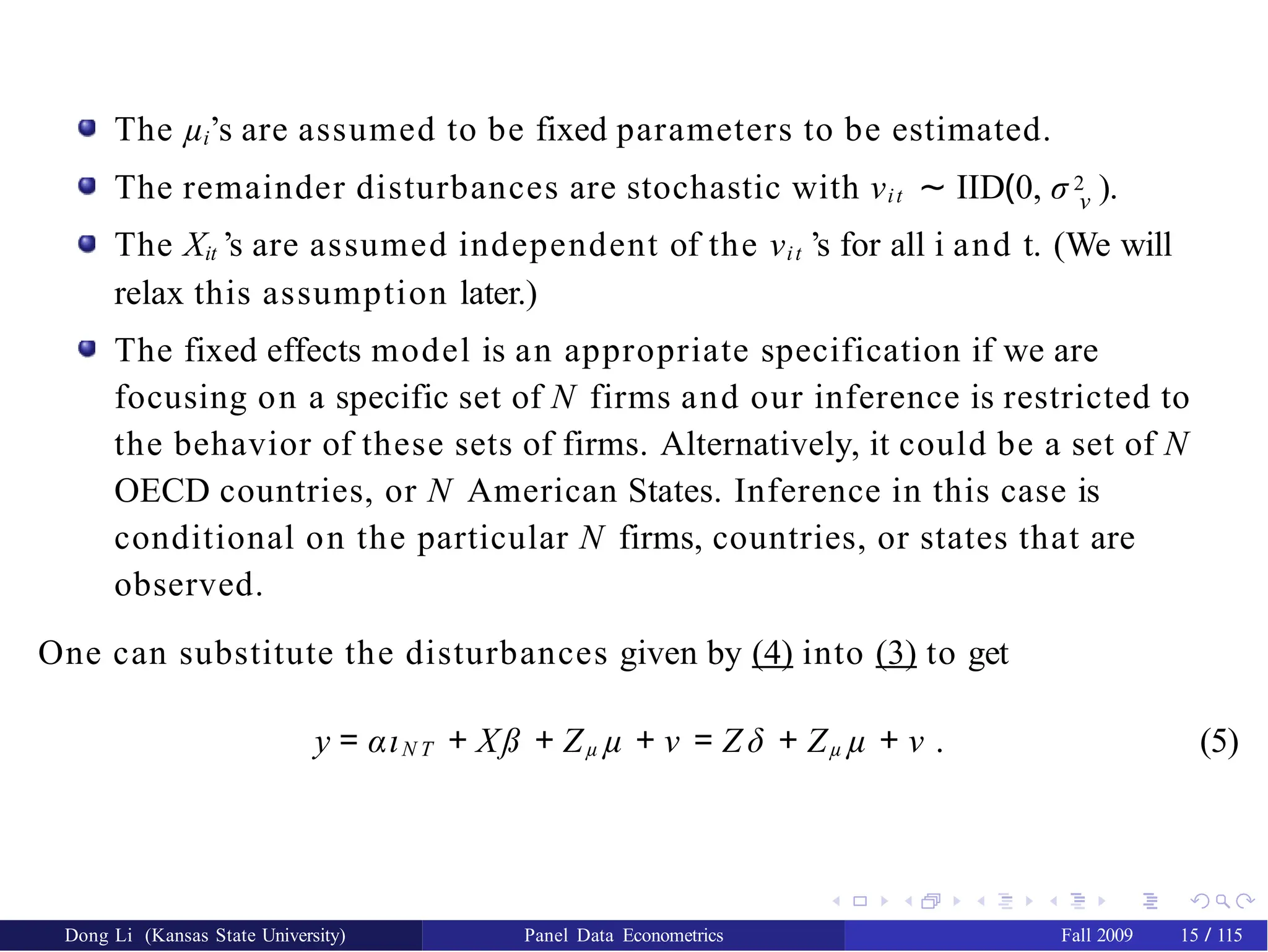
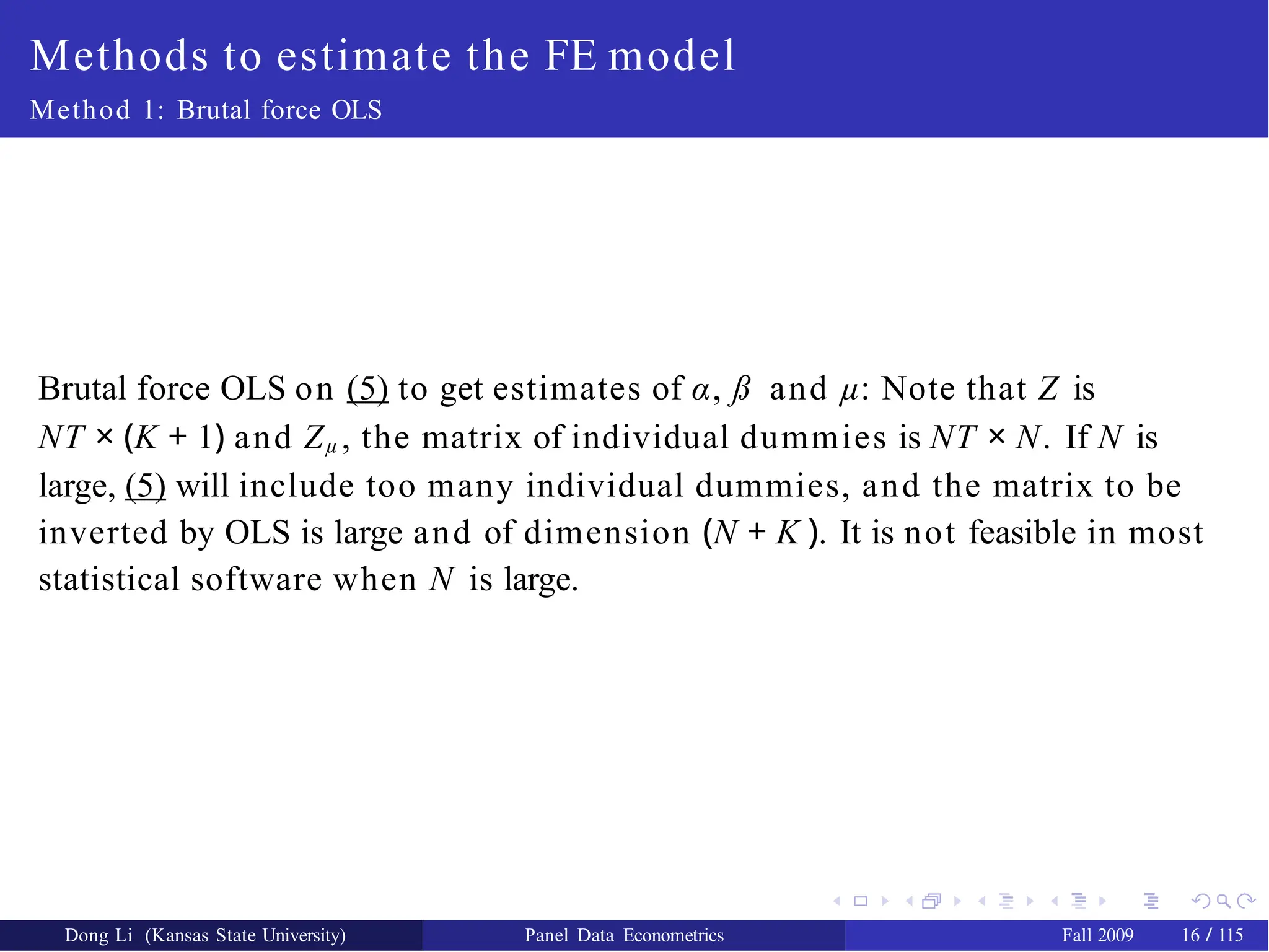
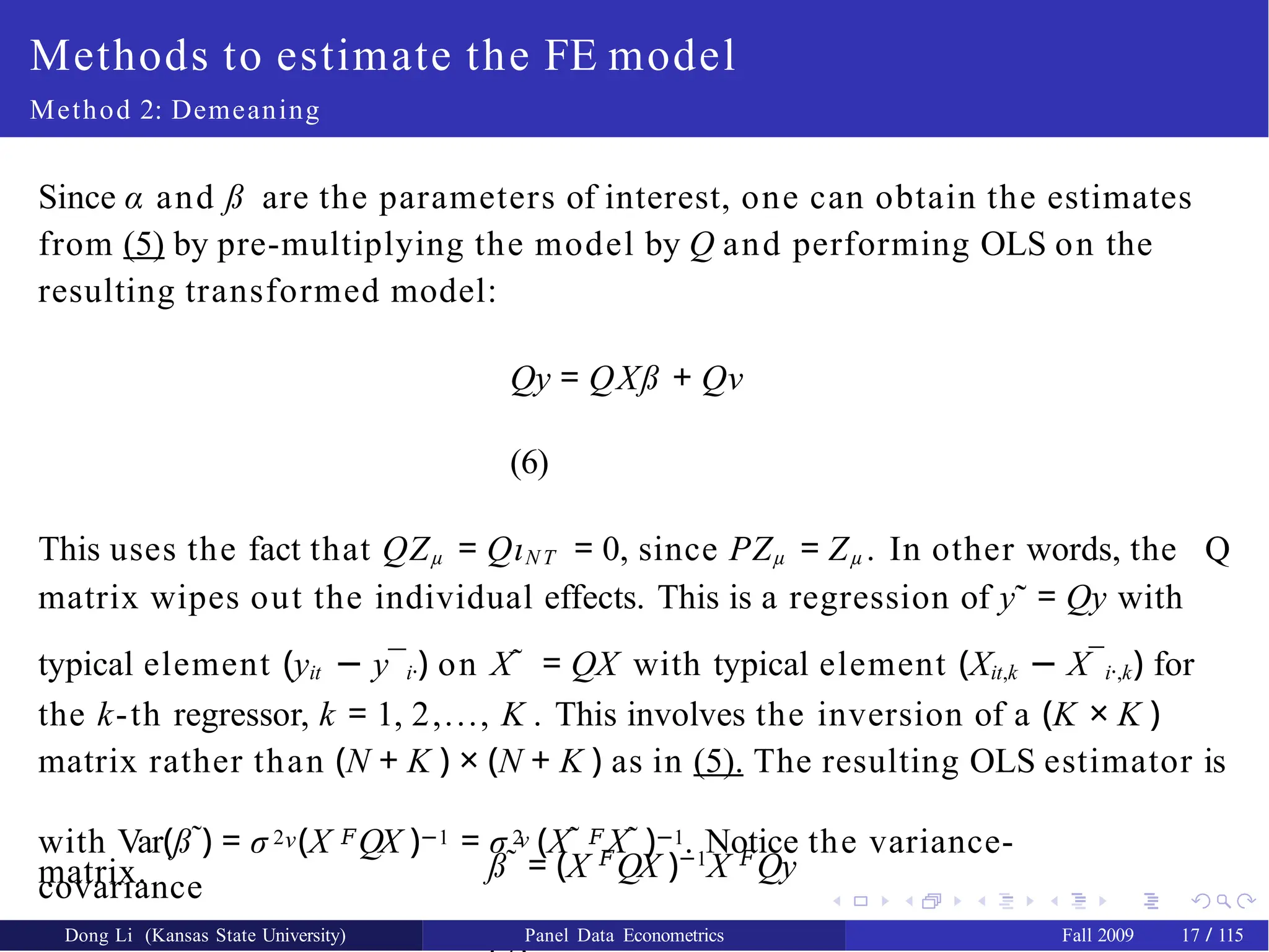
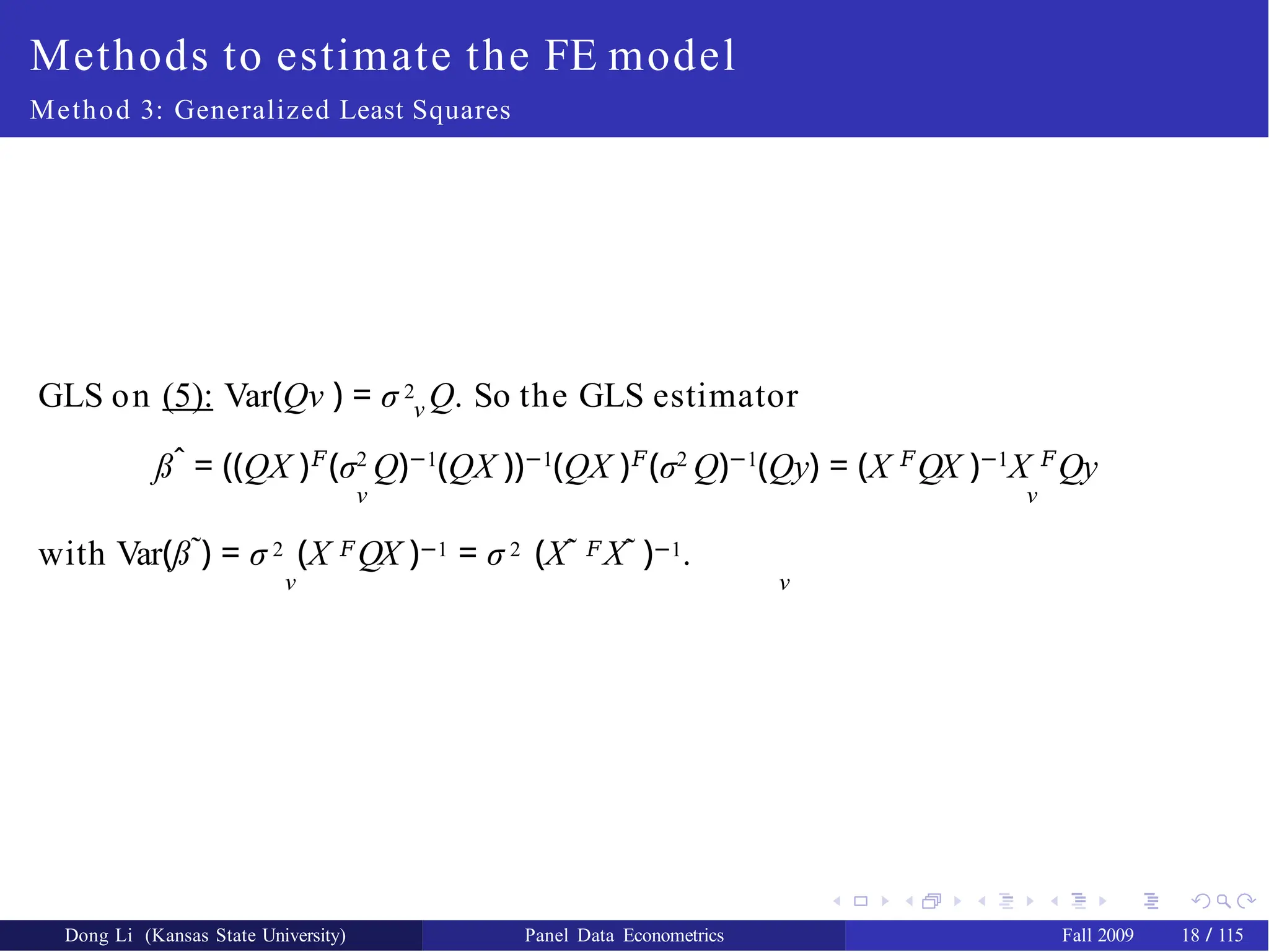
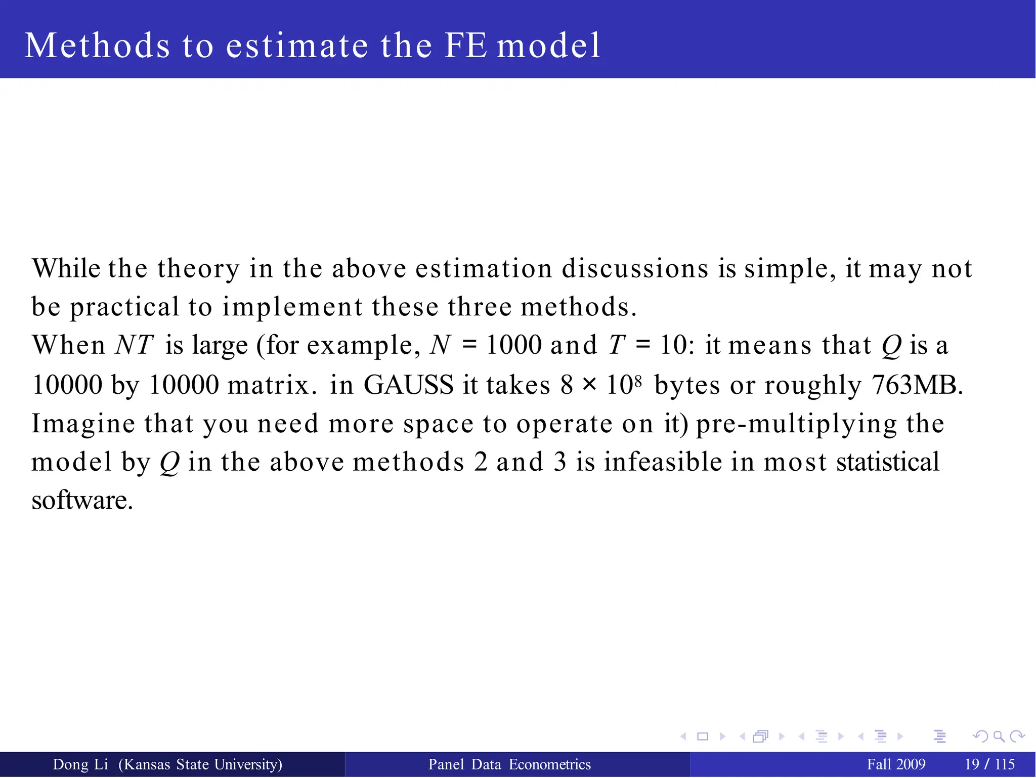
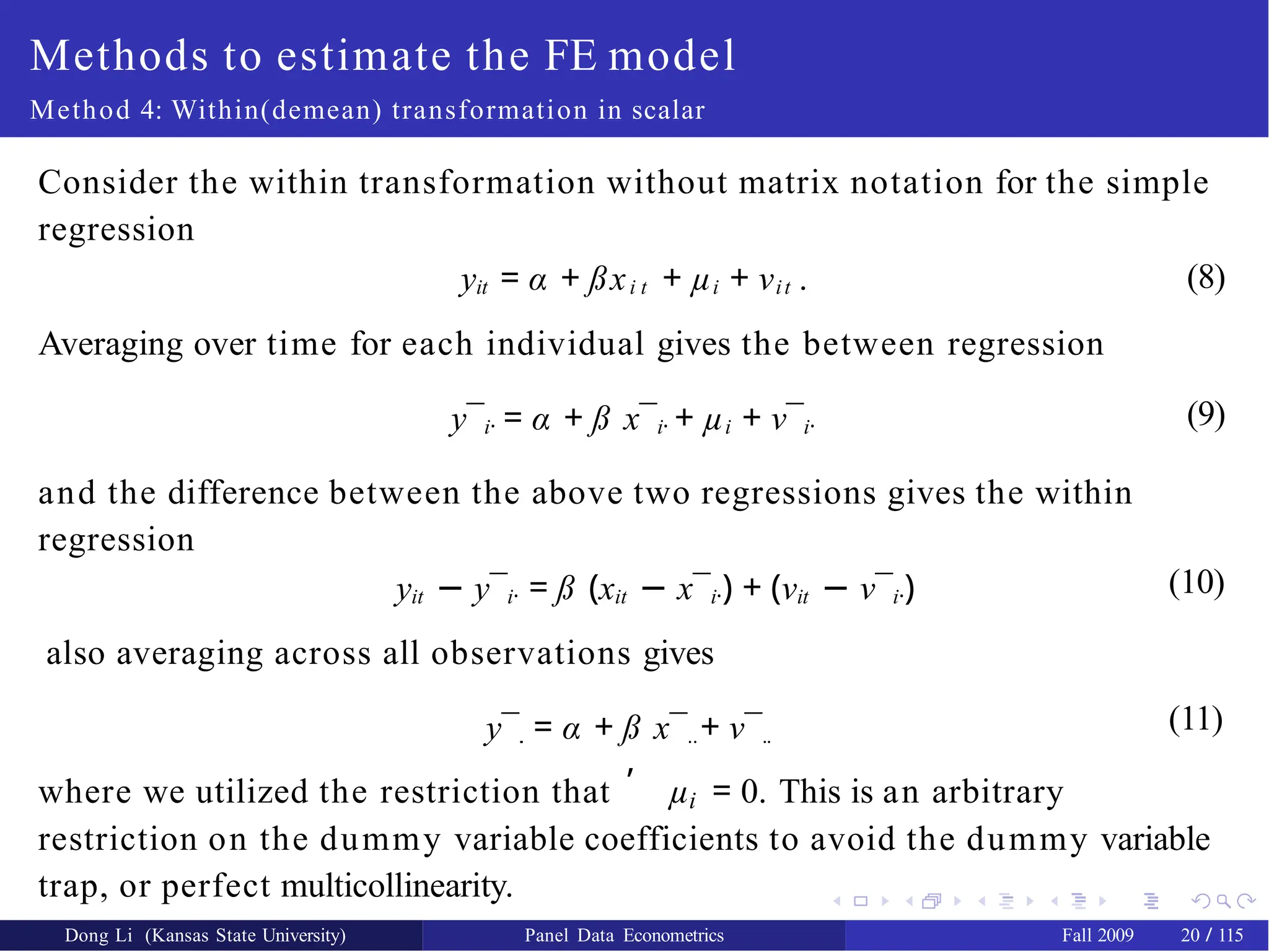
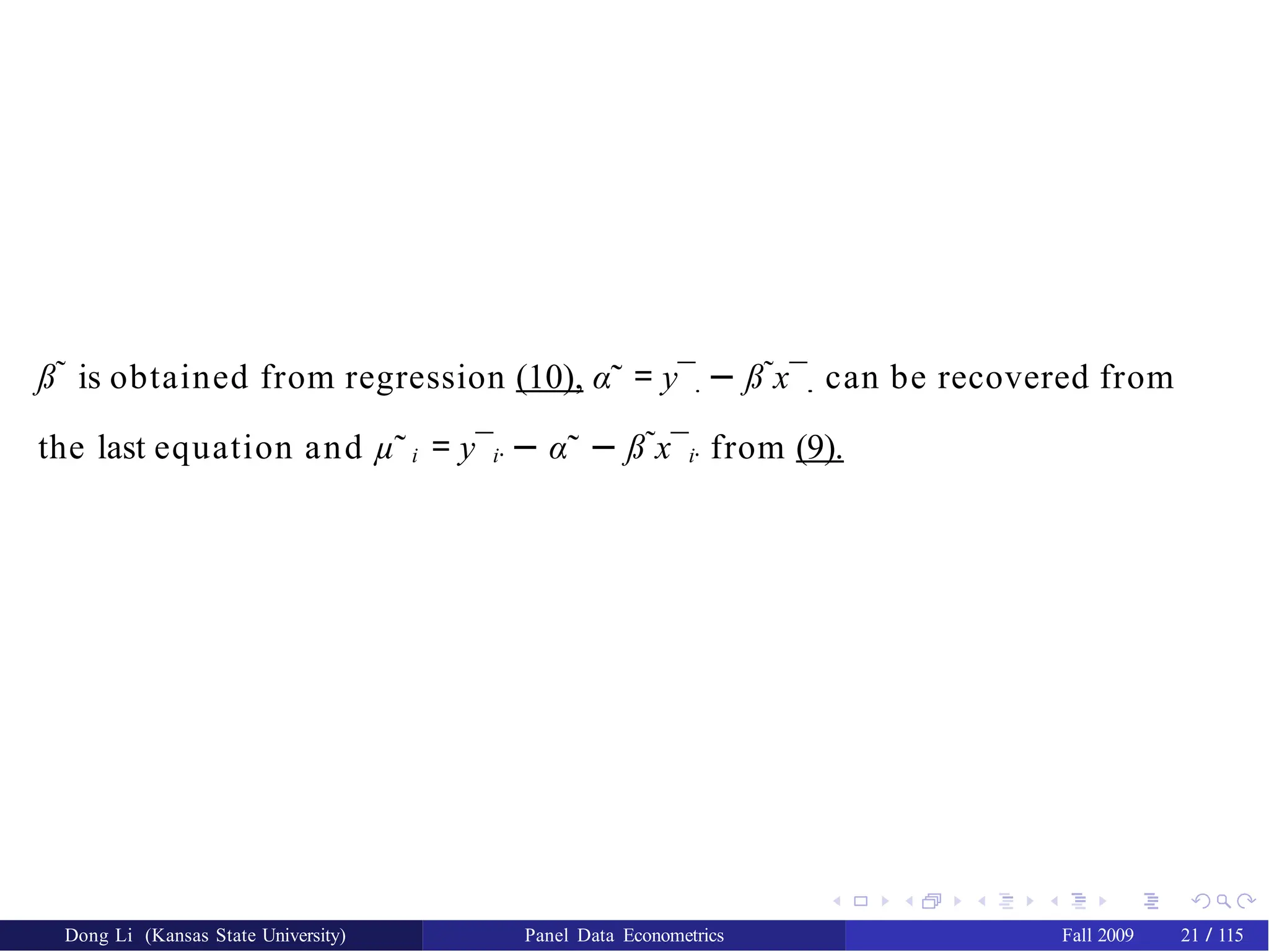
![A few comments
1 Testing for fixed effects. One could test the joint significance of these
dummies, i.e., H0: µ1 = ... = µN − 1 = 0, by performing an F test. This is a
simple F test with the RRSS being that of OLS on the pooled model
and the URSS being that of the LSDV regression.
F =
(RRSS − URSS)/(N −
1)
URSS/(NT − N − K )
H0
∼ FN−1,N(T −1)−K (12)
This test is available after FE regression in Stata.
Computational Warning. One computational caution for those using
the within regression given by (10). The s2 of this regression as
obtained from a typical regression package divides the residual sums
of squares by NT − K since the intercept and the dummies are not
included. The proper s2, say s∗2 from the LSDV regression would divide
the same residual sums of squares by N(T − 1) − K . Therefore, one has
to adjust the variances obtained from the within regression (10) by
multiplying the variance-covariance matrix by (s∗2/s2) or simply by
multiplying by [NT − K ]/[N(T − 1) − K ].
2
Dong Li (Kansas State University) Panel Data Econometrics Fall 2009 23 / 115](https://image.slidesharecdn.com/panelppt-250531033225-958aba86/75/panel-data-analysis-with-implications-and-importance-25-2048.jpg)
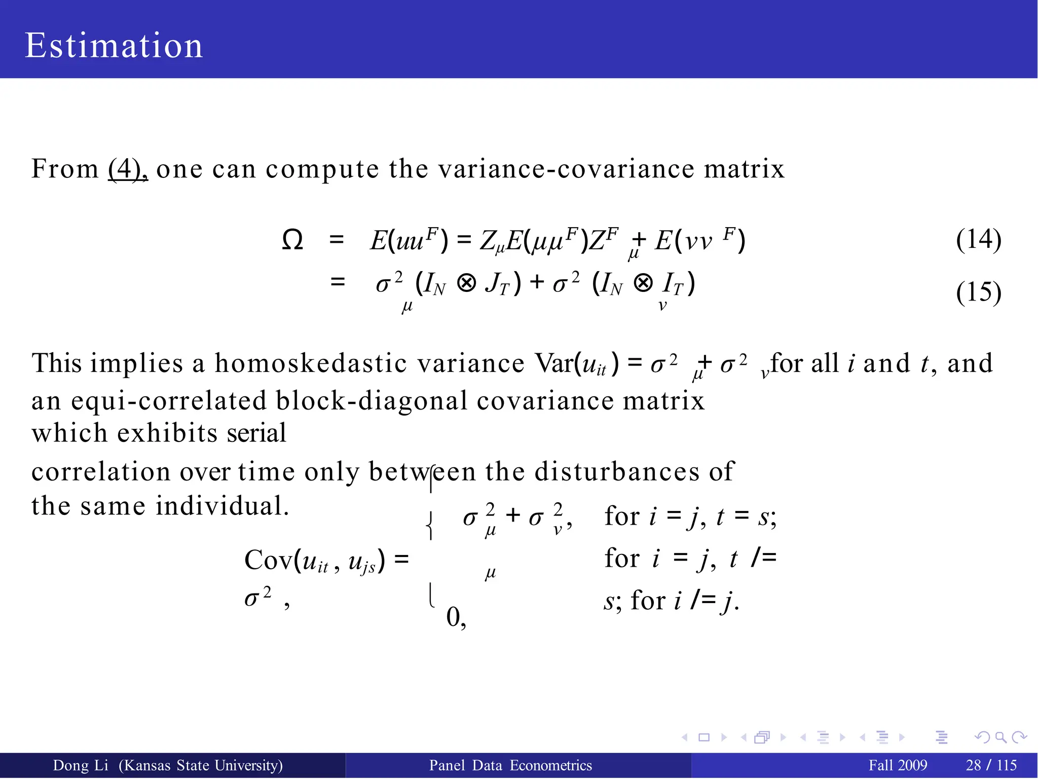
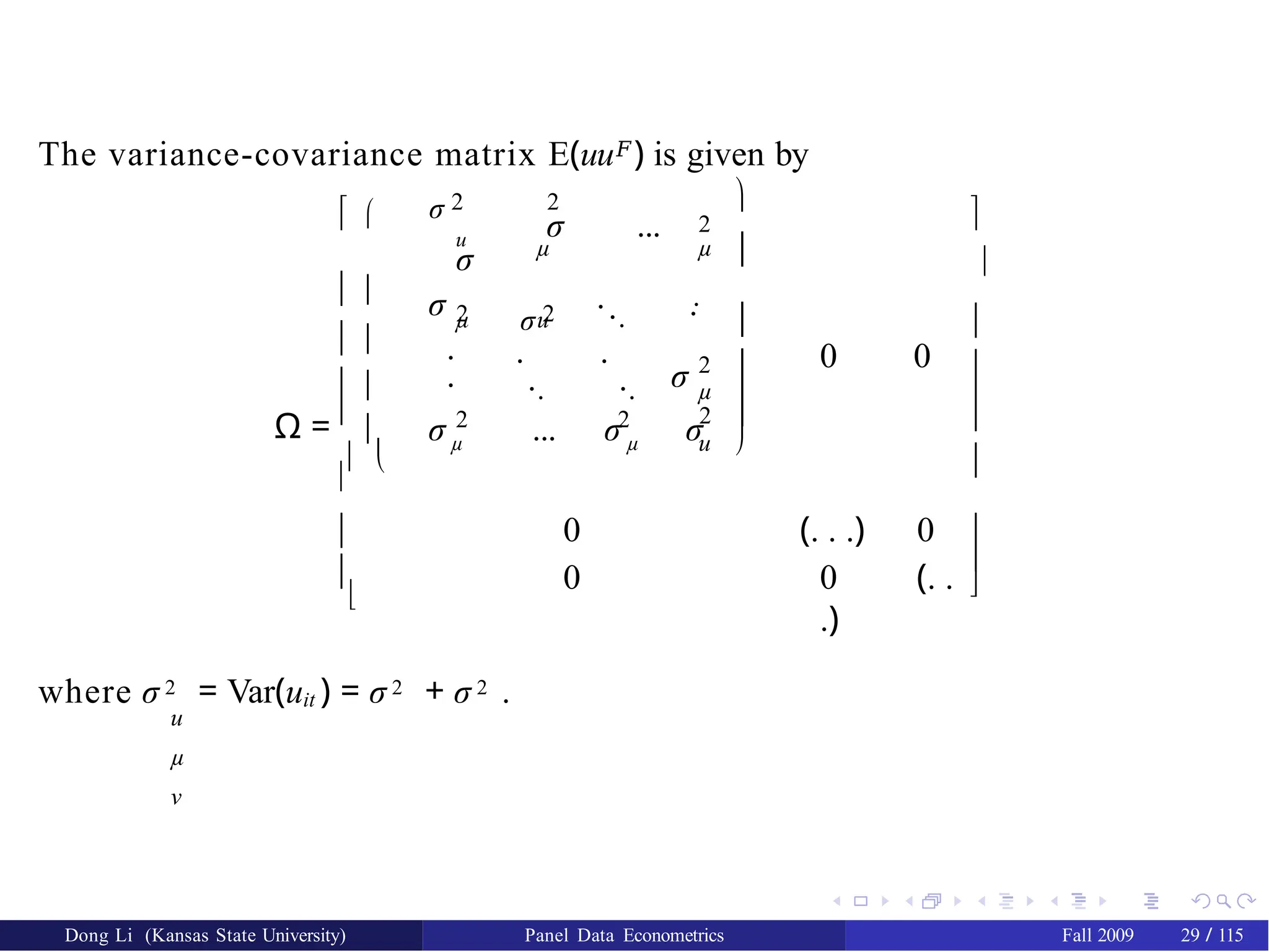
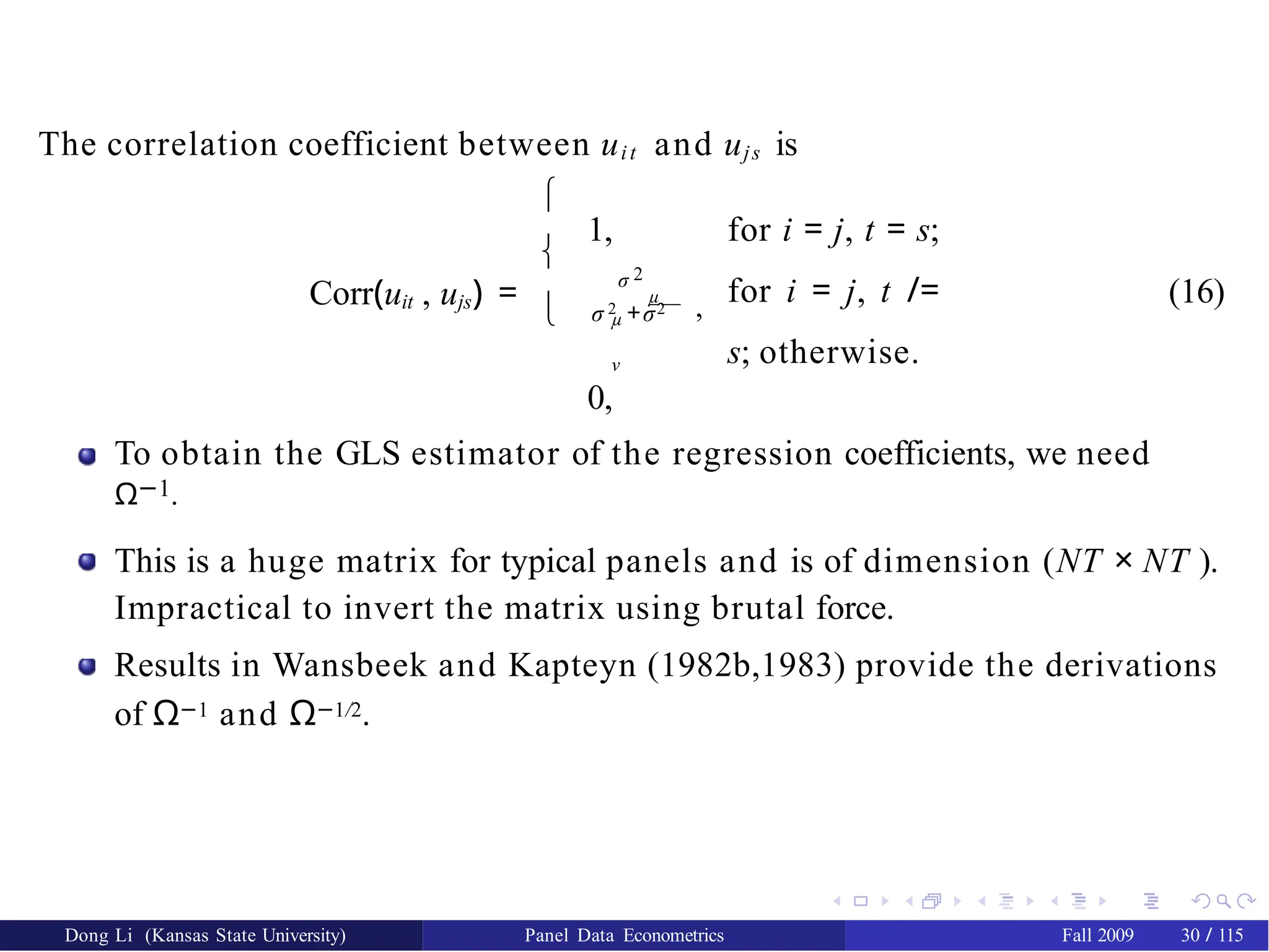
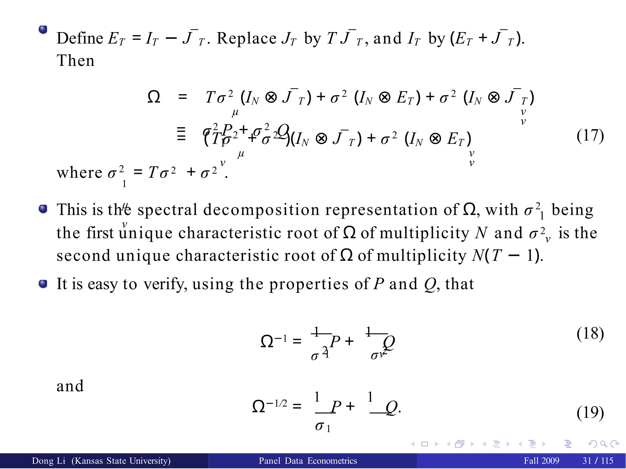
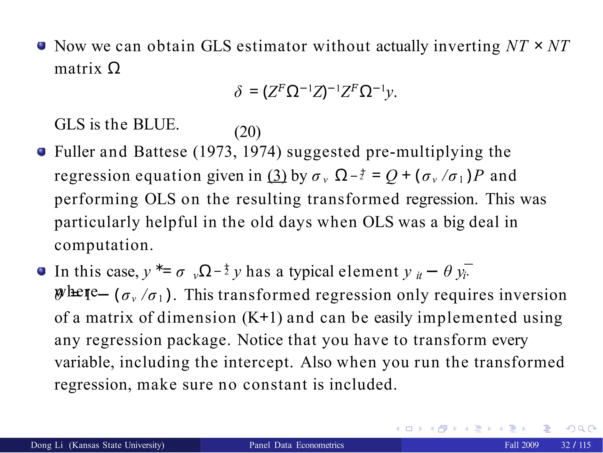
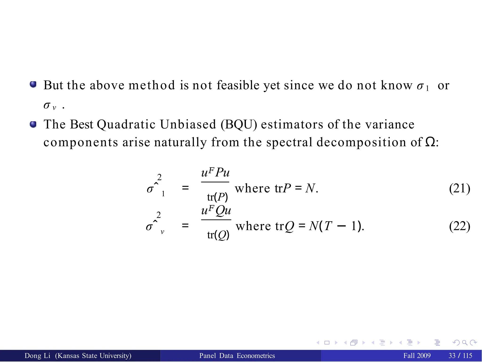
![We can show that the above estimators are unbiased.
E(u𝐹
Qu) = E(tr(u𝐹
Qu)) = E(tr(uu𝐹
Q)) = tr(E(uu𝐹
Q)) = tr(E(uu𝐹
)Q)
= tr(ΩQ) = tr[(σ2
P + σ 2
Q)Q] = tr(σ2
Q) = σ 2
trQ
1
ν
ν
ν
So
ν
E(σˆ 2
) = E
�
�
u Qu
= ν
σ 2 tr(Q)
tr(Q) tr(Q)
Dong Li (Kansas State University) Panel Data Econometrics Fall 2009 34 / 115
ν
= σ 2
.
Similar results can be obtained for σˆ 2
.
1
The true disturbances u are not known and therefore (21) and (22) are not
feasible. How to estimate u (uˆ) to make the GLS feasible (FGLS)?](https://image.slidesharecdn.com/panelppt-250531033225-958aba86/75/panel-data-analysis-with-implications-and-importance-36-2048.jpg)
![Ways to estimate the error components:
1 Wallace and Hussain (1969) suggest substituting OLS residuals
uˆOLS instead of the true u’s, because the OLS estimates are still
unbiased and consistent, though no longer efficient.
Amemiya (1971) shows that the Wallace and Hussain estimators of the
variance components have a different asymptotic distribution from
that knowing the true disturbances. He suggests using the LSDV
residuals instead of the OLS residuals.
Swamy and Arora (1972) suggest running two regressions to get
estimates of the variance components from the corresponding mean
square errors of these regressions. The first regression is the Within
regression which yields
2
3
σ
^
2
ν
𝐹 𝐹 𝐹
−1 𝐹
= [y Qy − y QX (X QX ) X Qy]/[N(T − 1) − K ]. The
second
regression is the Between regression which yields
σ
^
2
𝐹
1
𝐹
𝐹
= [y Py − y PZ(Z PZ −1
𝐹
) Z Py]/(N − K −
1
).
4 2
, N
µ i=1
¯ 2
Nerlove (1971) suggests σˆ = (µˆ − µˆ) /(N
− 1
i i
) where µˆ are the
ν
dummy coefficients estimates from the LSDV regression. σˆ 2 is
estimated from the within residual sums of squares divided by NT
without correction for degrees of freedom.
Dong Li (Kansas State University) Panel Data Econometrics Fall 2009 35 / 115](https://image.slidesharecdn.com/panelppt-250531033225-958aba86/75/panel-data-analysis-with-implications-and-importance-37-2048.jpg)
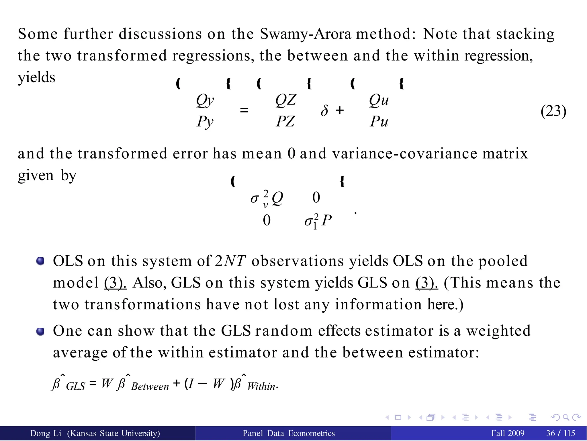
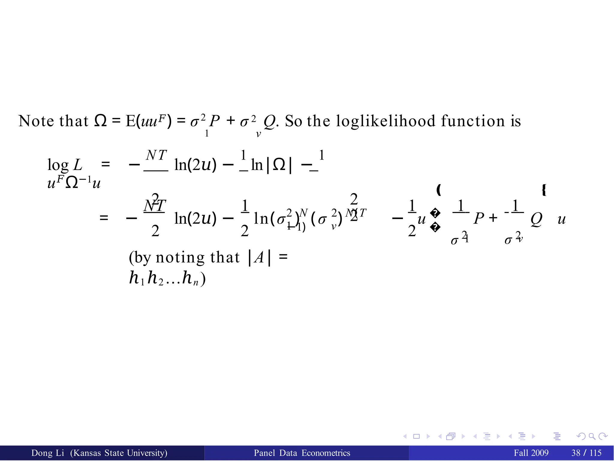
![If the (unobserved) individual effects µi’s are random, the error terms
uit are autocorrelated (but homoscedastic). The OLS estimators are
still unbiased, but not efficient. The OLS standard errors are
misleading.
If the (unobserved) individual effects µi’s are fixed and we run OLS
without µ in the regression, it causes the omitted variable problem
(omission of relevant variables). The OLS estimators are biased.
If the true model is y = Xß + Zγ + u but we estimate y = Xß + u instead
(ߘ = (X 𝐹X )−1X 𝐹y), we have
ߘ = (X 𝐹
X )−1
X 𝐹
(Xß + Z γ + u)
= ß + (X 𝐹
X )−1
X 𝐹
Zγ + (X 𝐹
X )−1
X
𝐹
u
So
E(ߘ) = ß + E[(X 𝐹
X )−1
X 𝐹
Z]γ + 0
(24)
The above expectation is not ß unless the second term is zero.
Dong Li (Kansas State University) Panel Data Econometrics Fall 2009 40 / 115](https://image.slidesharecdn.com/panelppt-250531033225-958aba86/75/panel-data-analysis-with-implications-and-importance-42-2048.jpg)
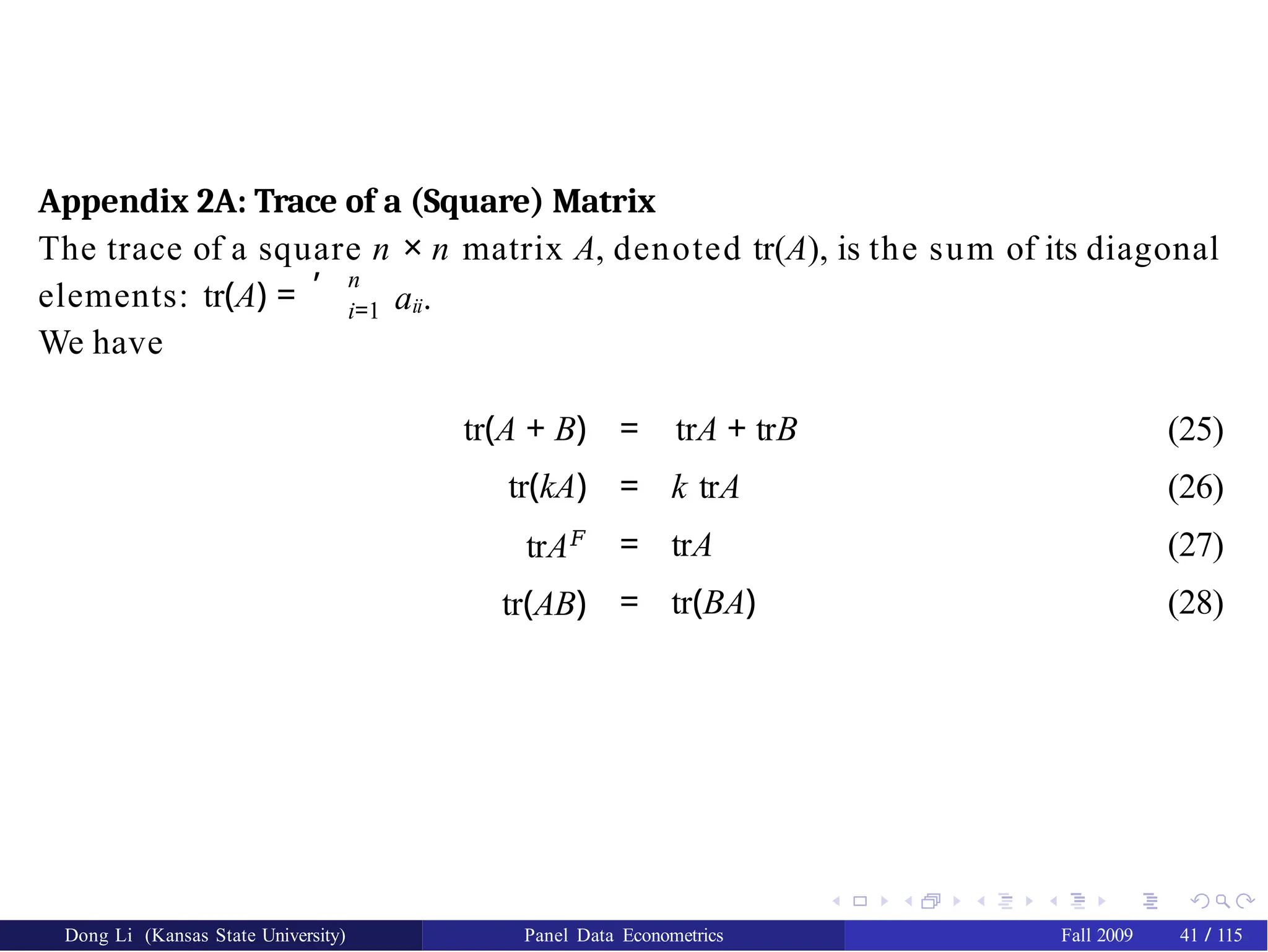


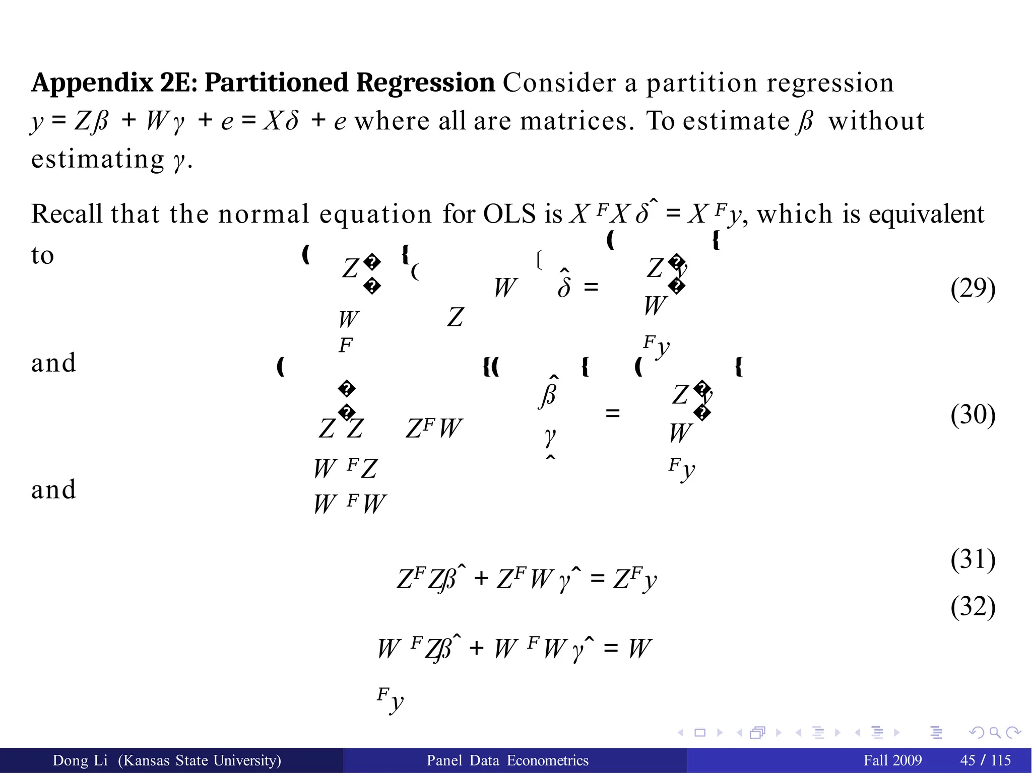
![From (32) one can find γˆ = (W 𝐹W )−1W 𝐹(y − Z߈). Plug this equation into
(31) one can obtain
Z𝐹
Z߈ + Z𝐹
W (W 𝐹
W )−1
W 𝐹
(y − Z߈) = Z𝐹
y
Z𝐹
Z߈ − Z𝐹
W (W 𝐹
W )−1
W 𝐹
Z߈ = Z𝐹
y − Z𝐹
W (W 𝐹
W )
−1
W 𝐹
y
Z𝐹
[I − W (W 𝐹
W )−1
W 𝐹
]Z߈ = Z𝐹
[I − W (W 𝐹
W )−1
W 𝐹
]y
(33)
(34)
(35)
Define PW = W (W 𝐹W )−1W 𝐹 and P¯ W = I − PW . PW is the projection
matrix and P¯ W is the residual projection. It is easy to verify that both PW
and P¯ W are symmetric and idempotent. The above equation becomes
(Z𝐹
P¯ W Z)߈ = Z𝐹
P¯ W y
߈ = (Z𝐹
P¯ W Z)−1
Z𝐹
P¯
W y
(36)
(37)
which is also the OLS estimator from the following regression
P¯ W y = P¯ W Zß + P¯ W e.
Dong Li (Kansas State University) Panel Data Econometrics Fall 2009 46 / 115](https://image.slidesharecdn.com/panelppt-250531033225-958aba86/75/panel-data-analysis-with-implications-and-importance-48-2048.jpg)
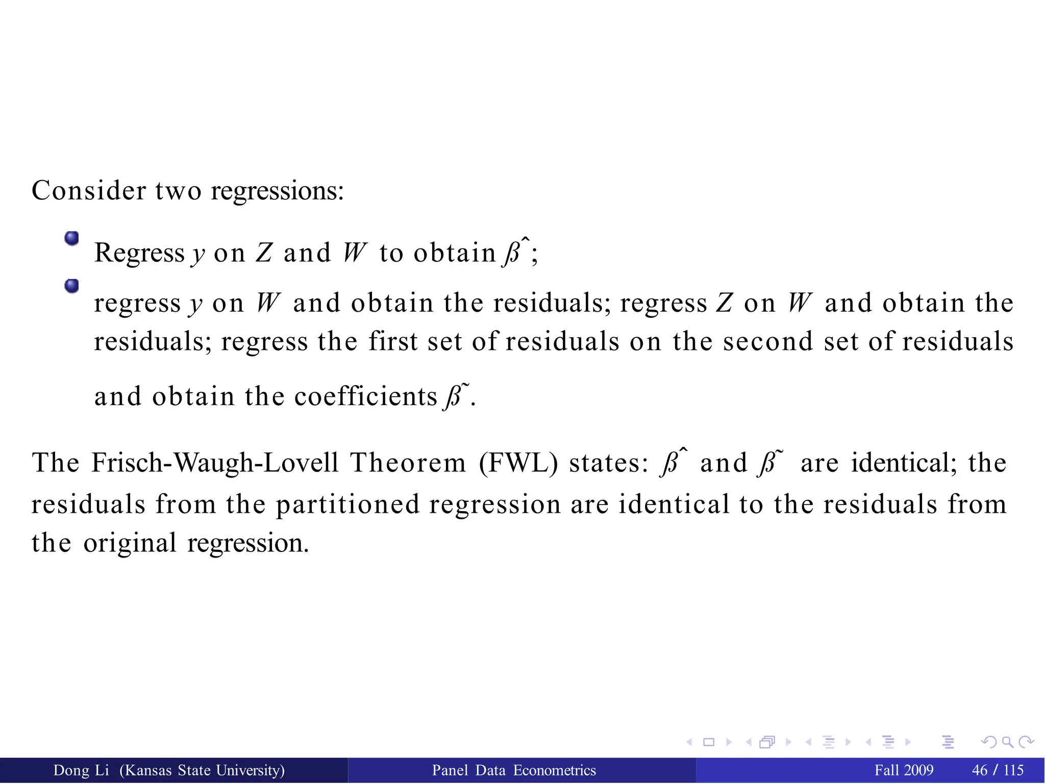

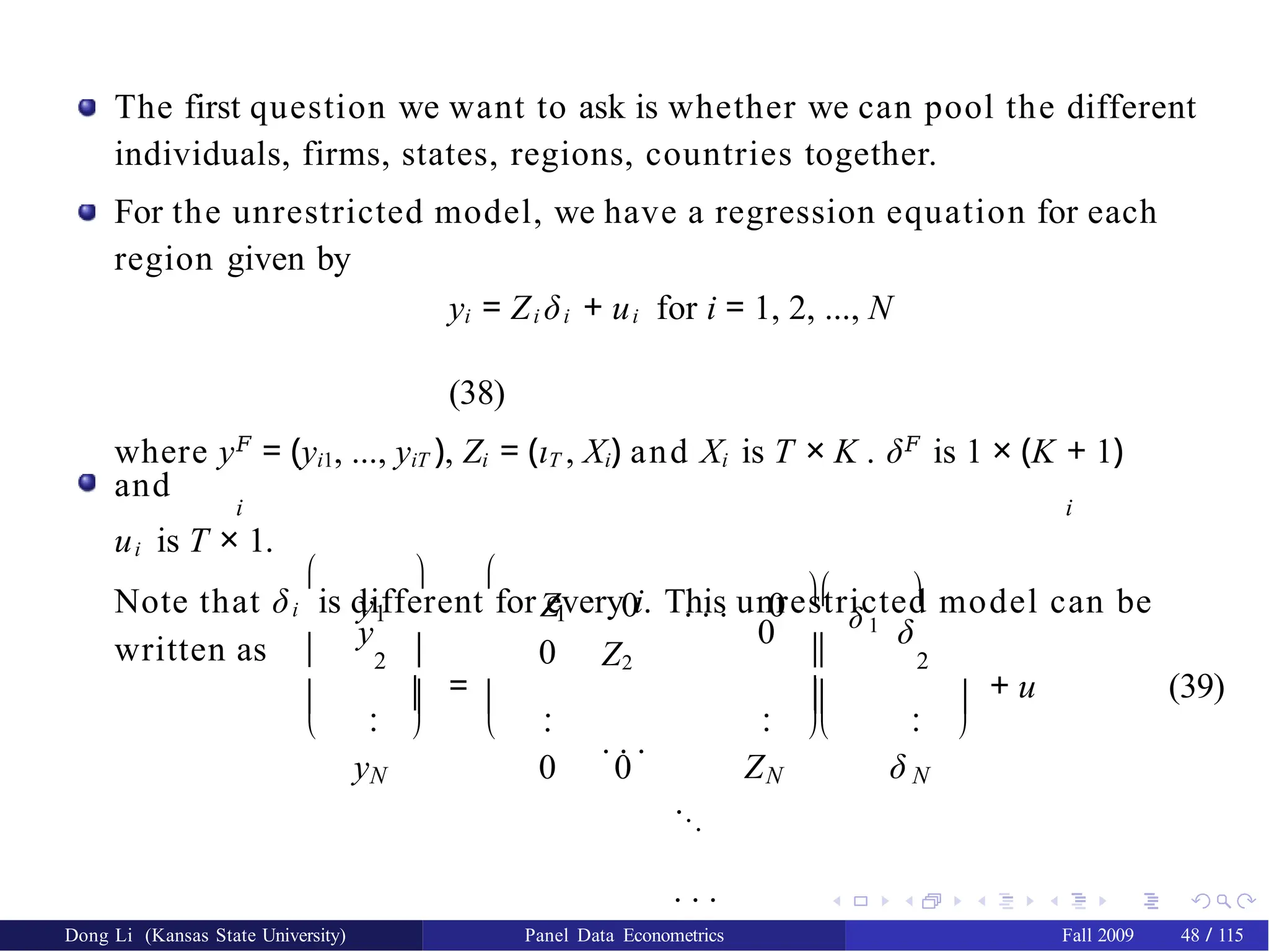
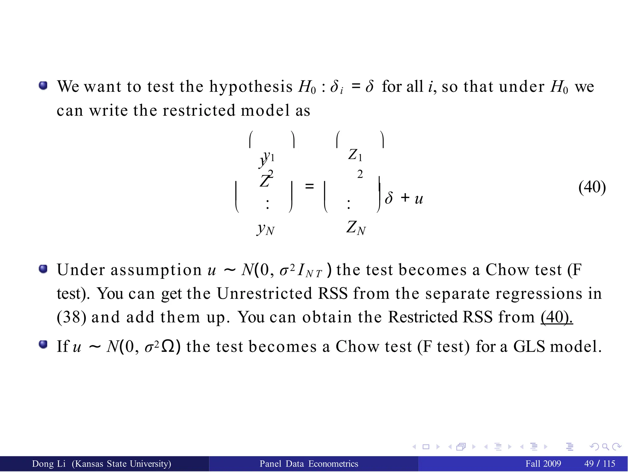
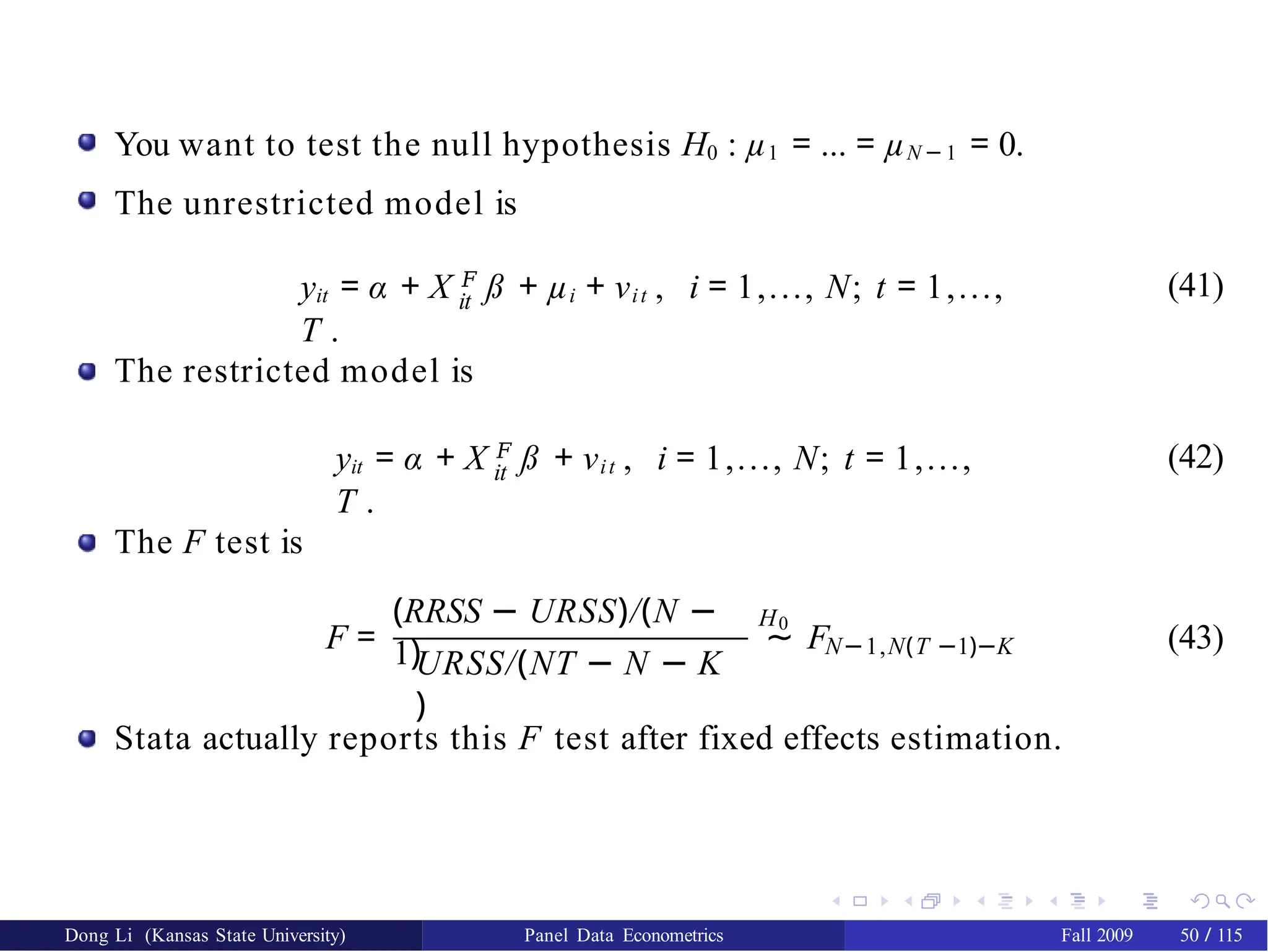
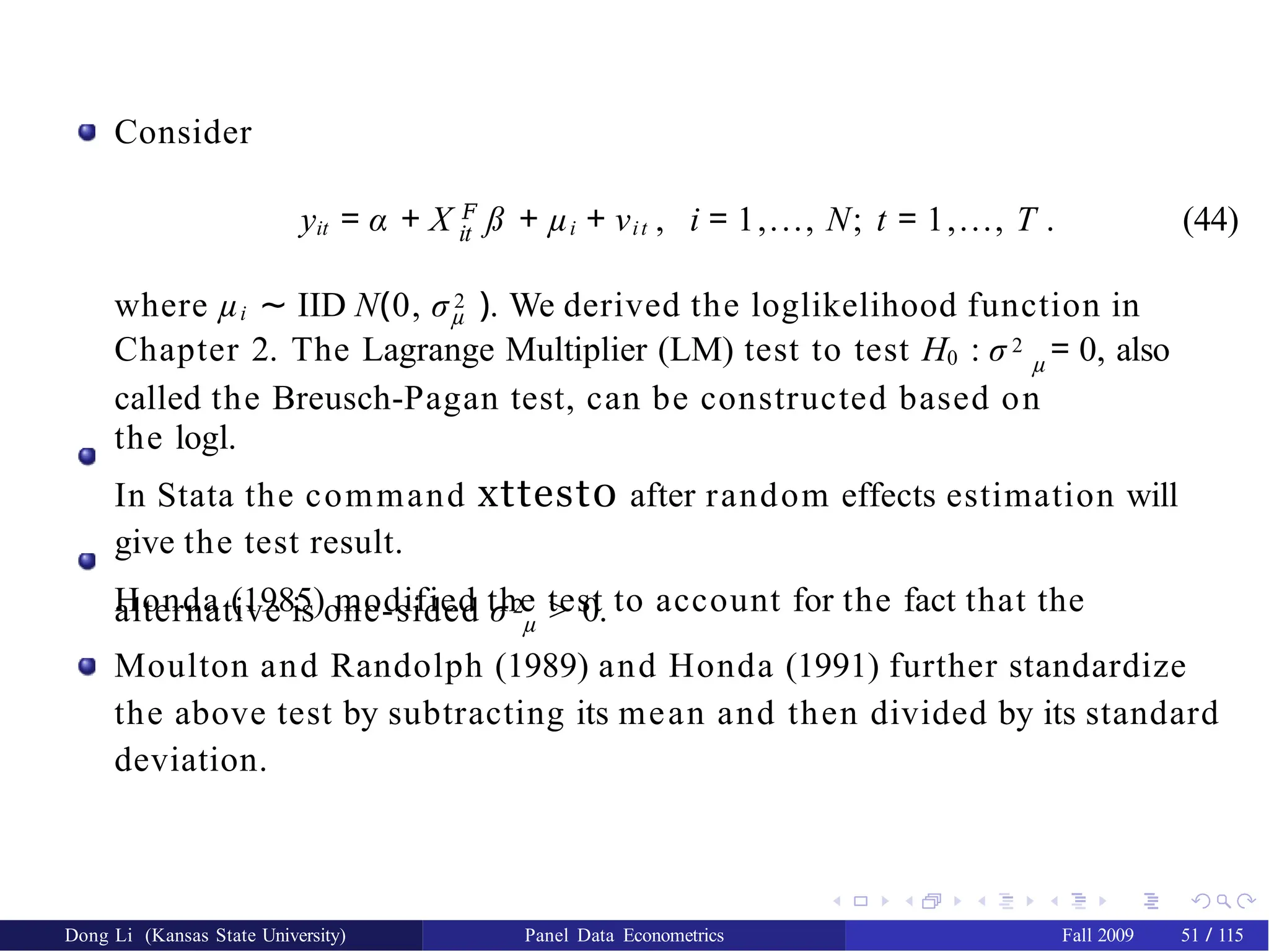
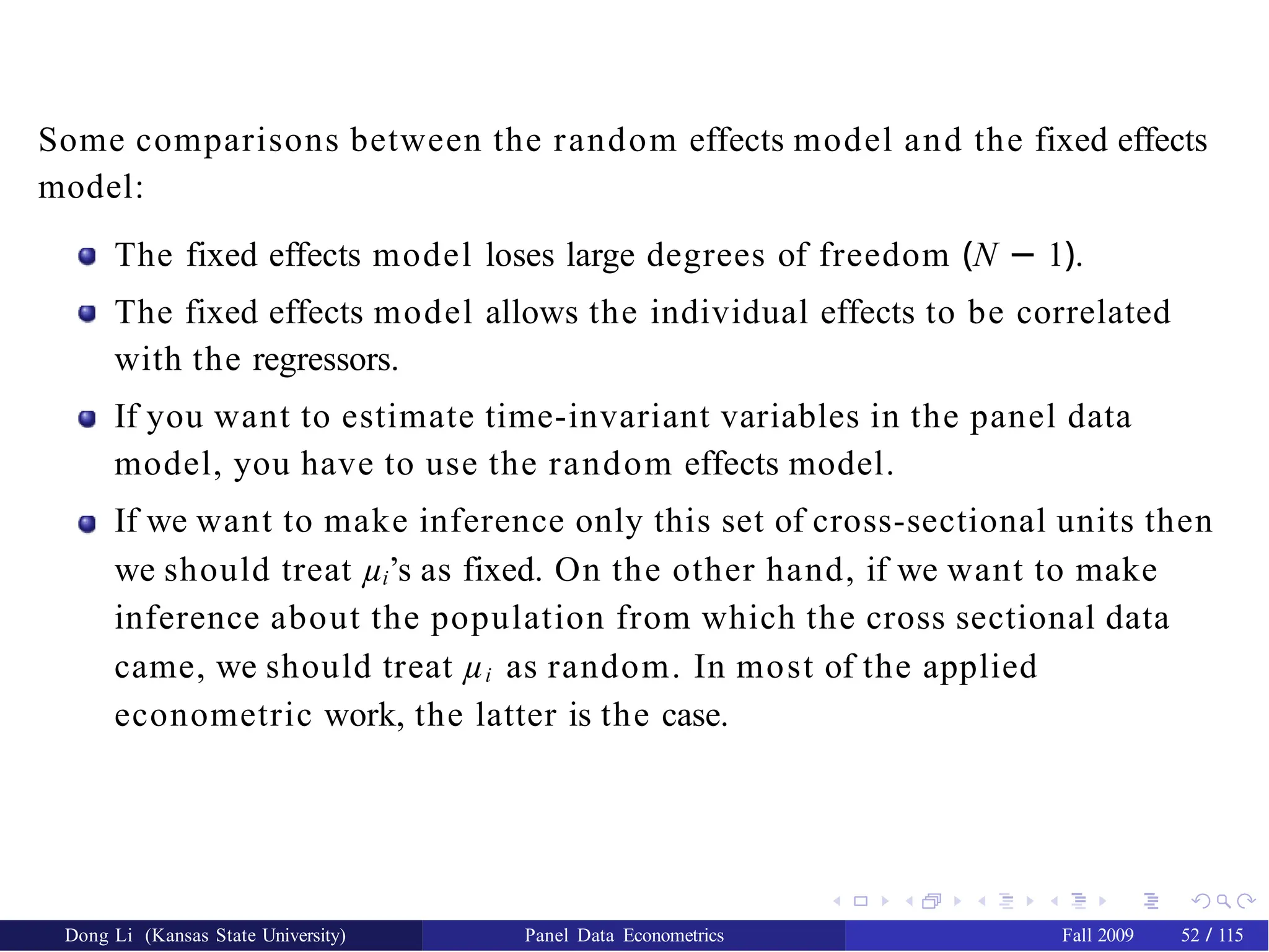

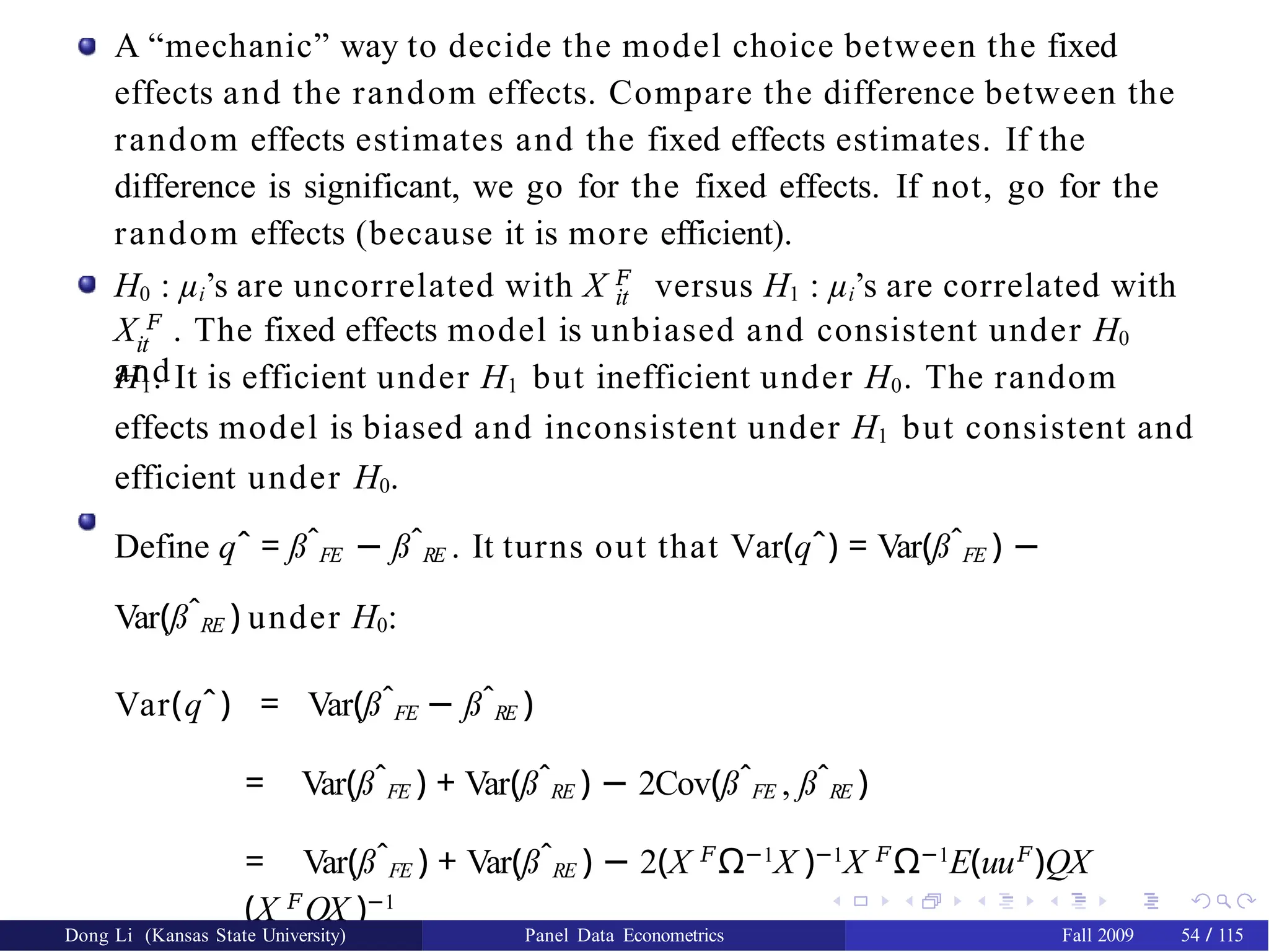
![The test statistic
m = qˆ𝐹
[Var(qˆ)]− 1
qˆ (45)
K
and under H0 it is asymptotically distributed as χ 2
, where K denotes the
dimension of slope vector.
xtreg lgaspcar lincomep lrpmg lcarpcap, re
est store random
xtreg lgaspcar lincomep lrpmg lcarpcap, fe
est store fixed
hausman fixed random
Note the order of the two estimates: hausman consistent
efficient
A pitfall of the Hausman test is that it may be negative in finite
samples.
Dong Li (Kansas State University) Panel Data Econometrics Fall 2009 55 / 115](https://image.slidesharecdn.com/panelppt-250531033225-958aba86/75/panel-data-analysis-with-implications-and-importance-58-2048.jpg)
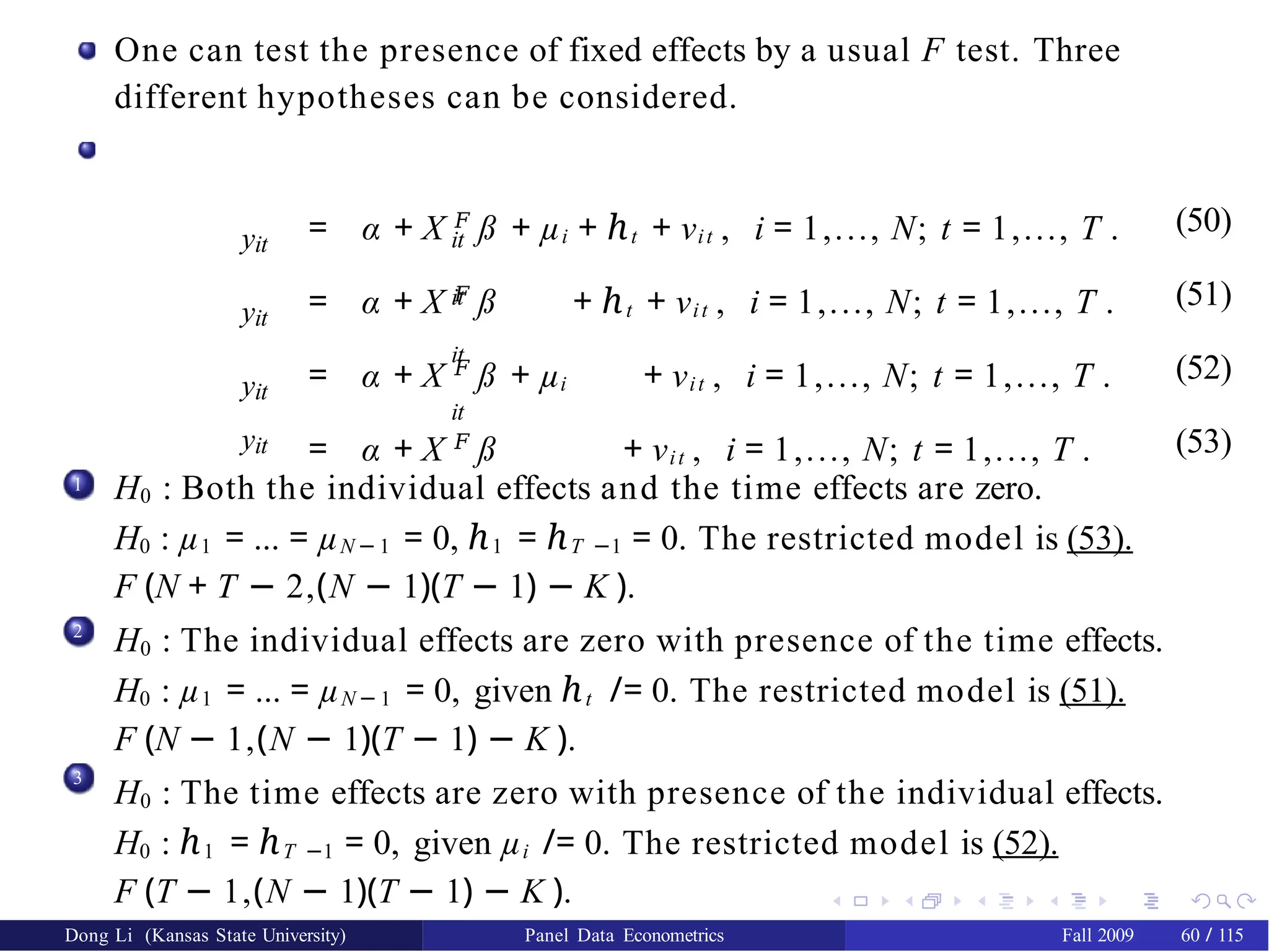
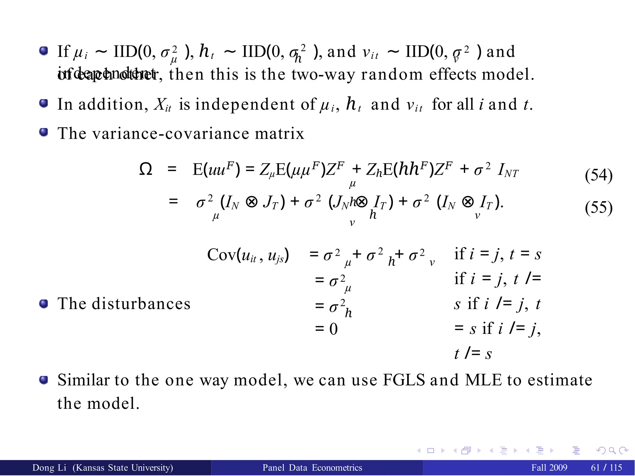
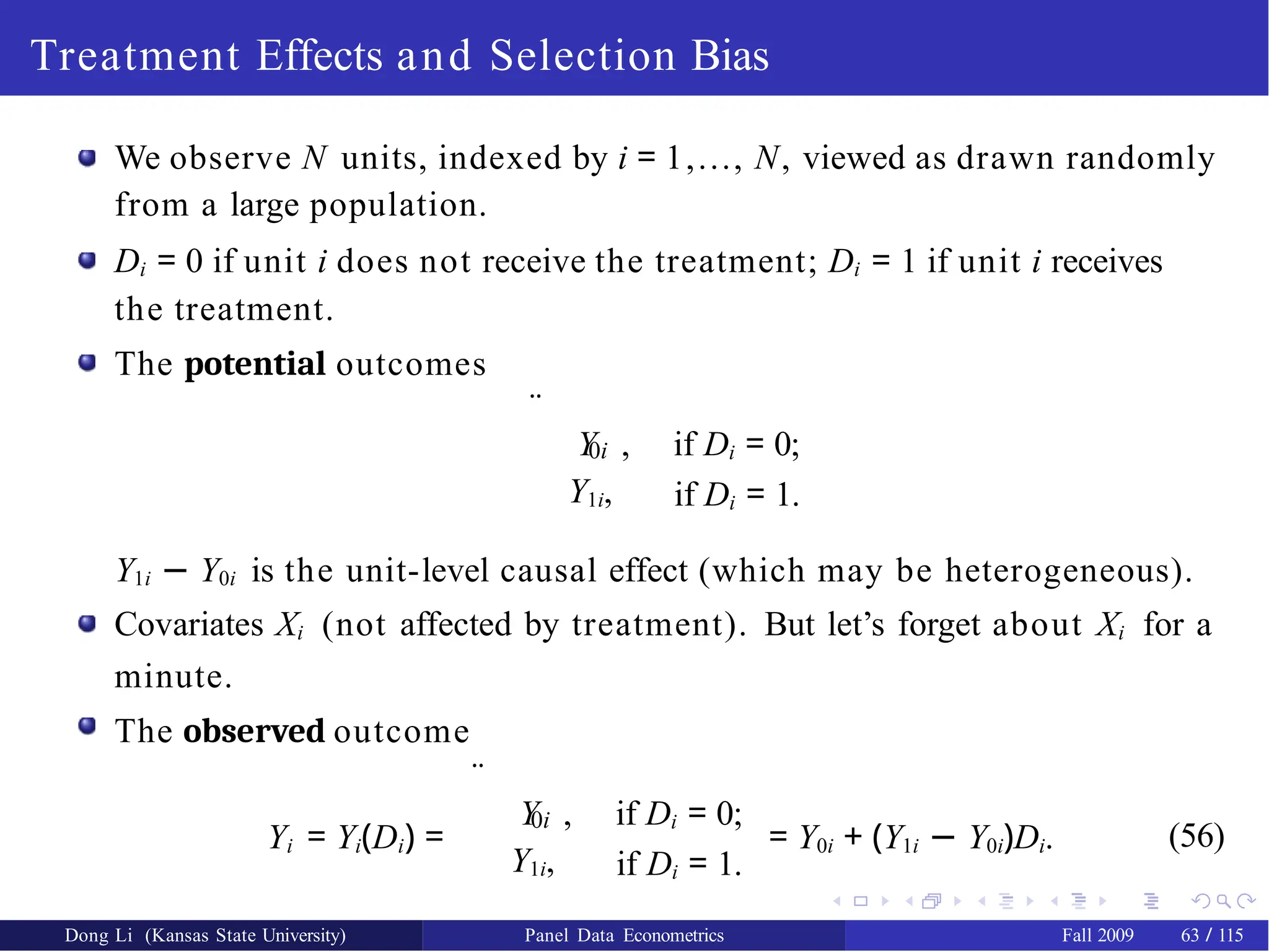
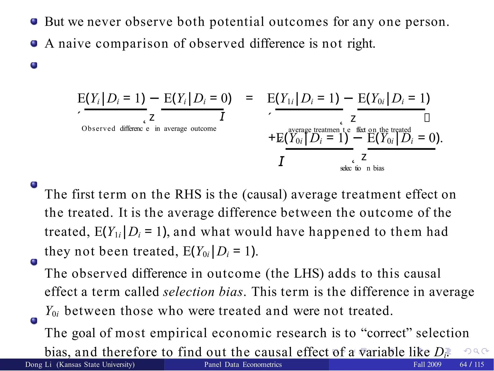
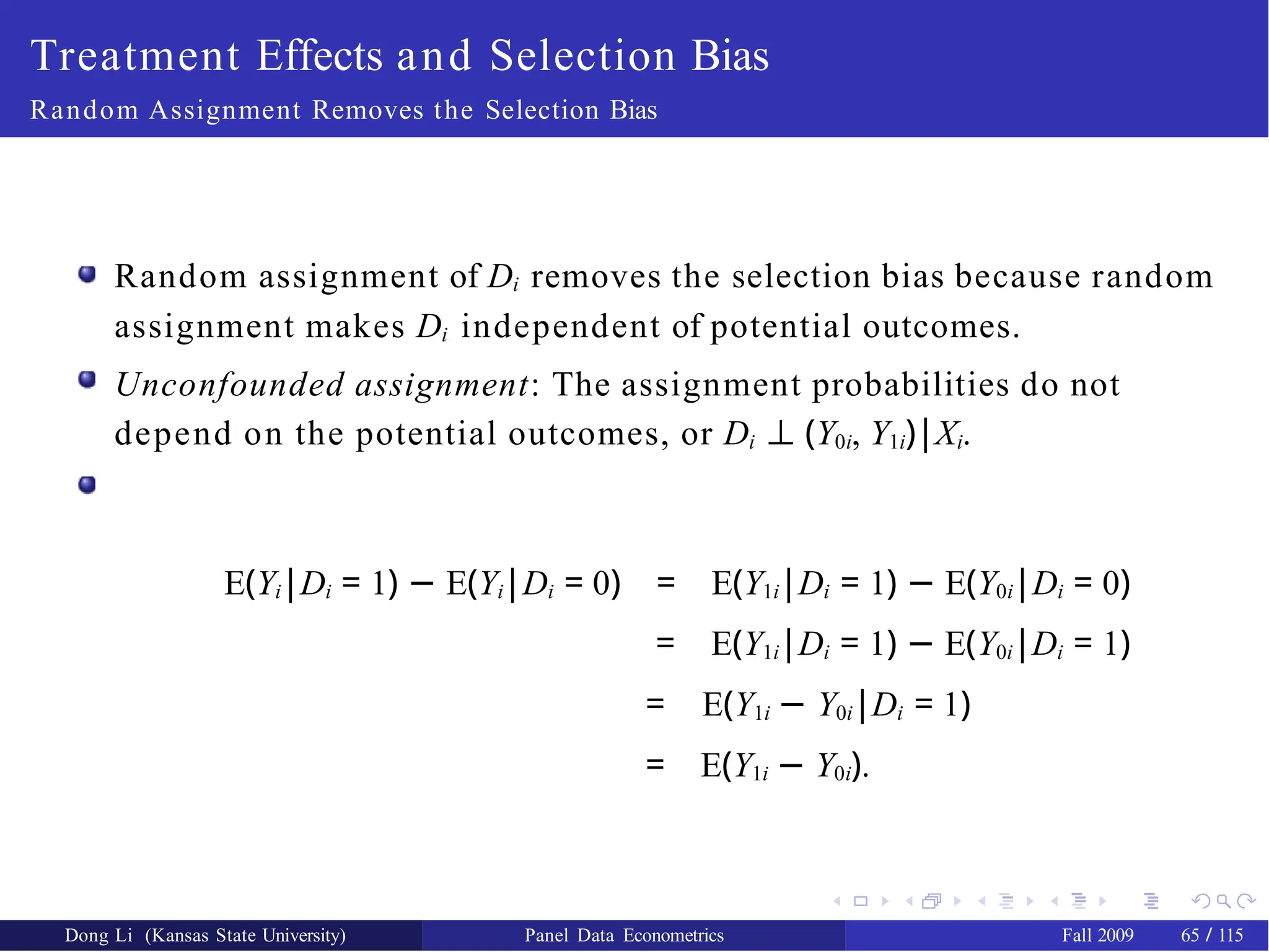

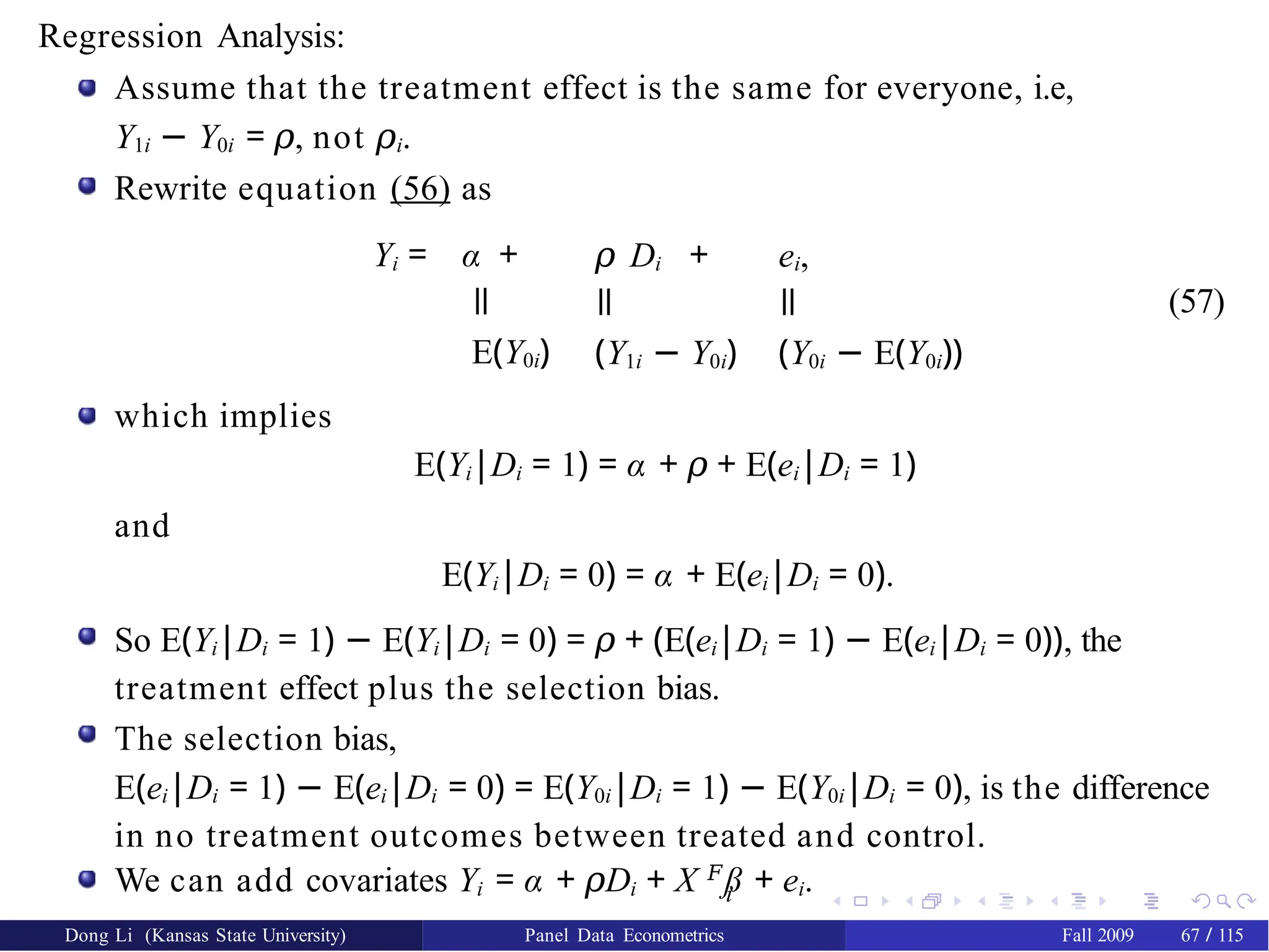
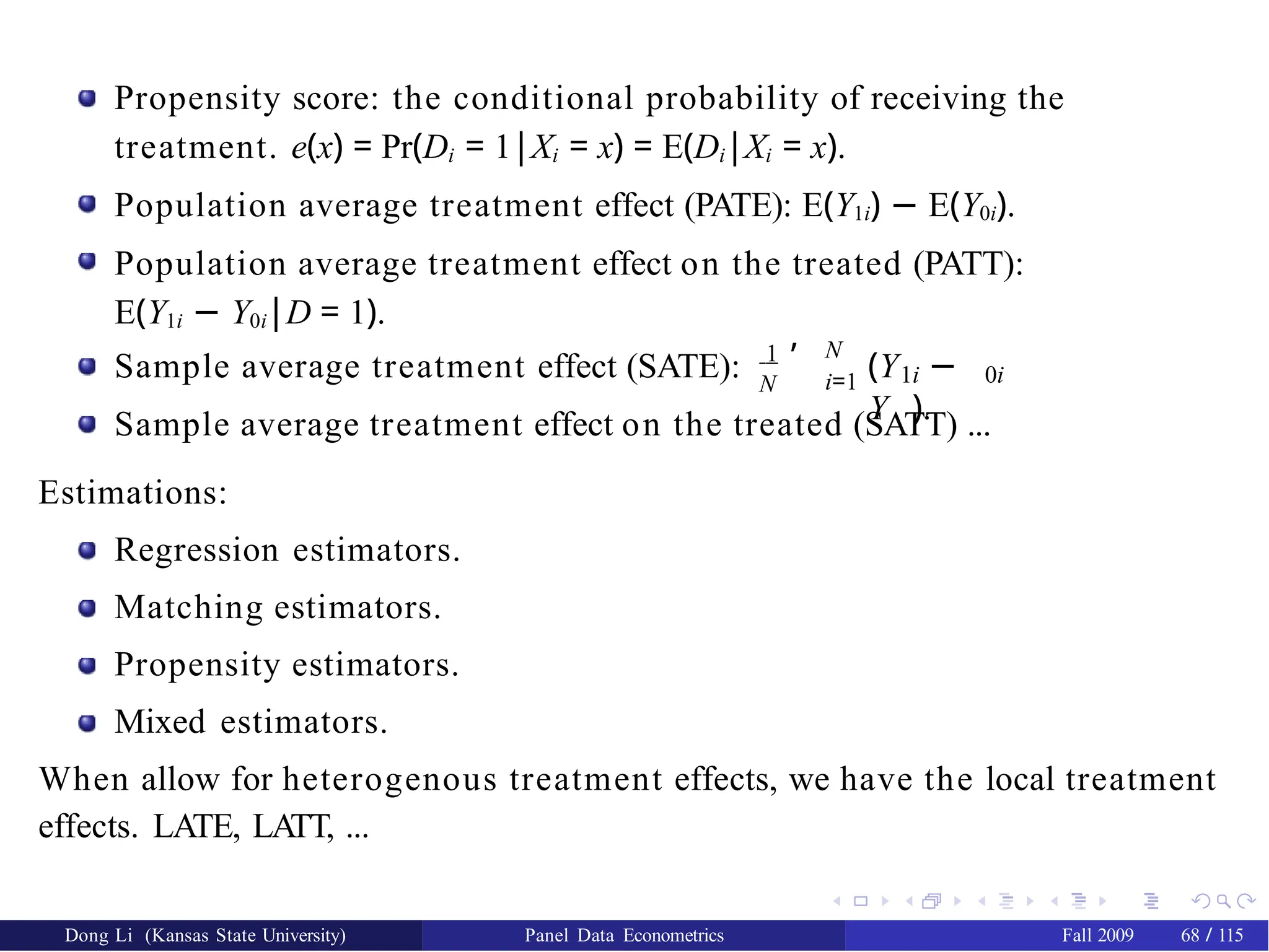
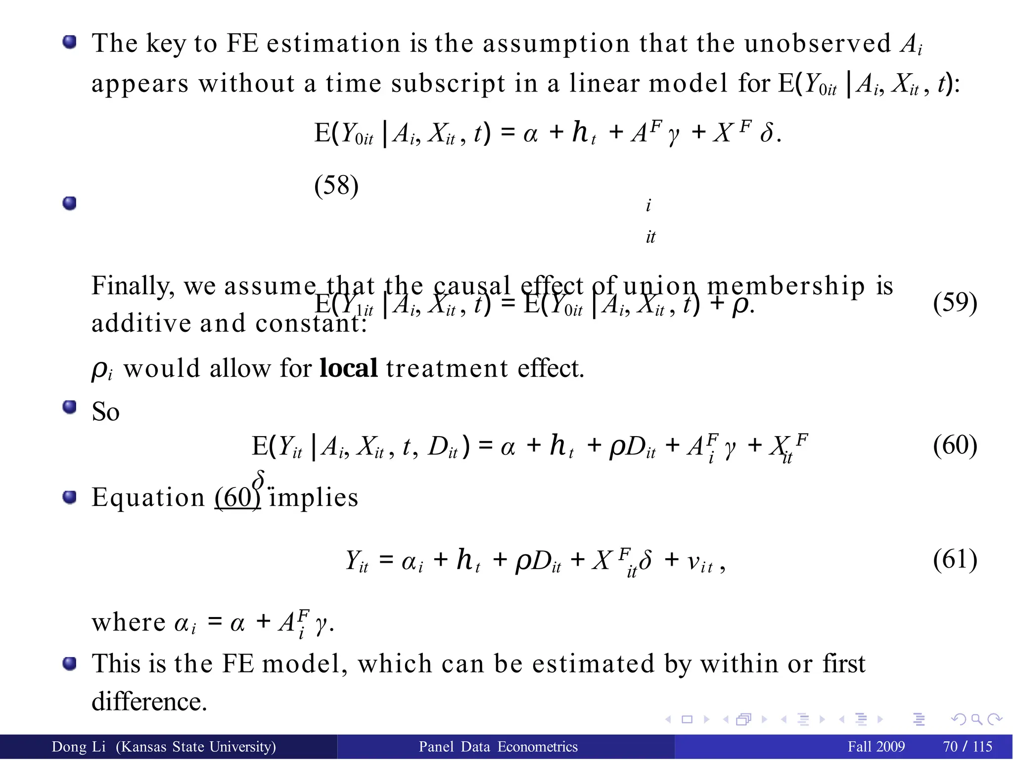
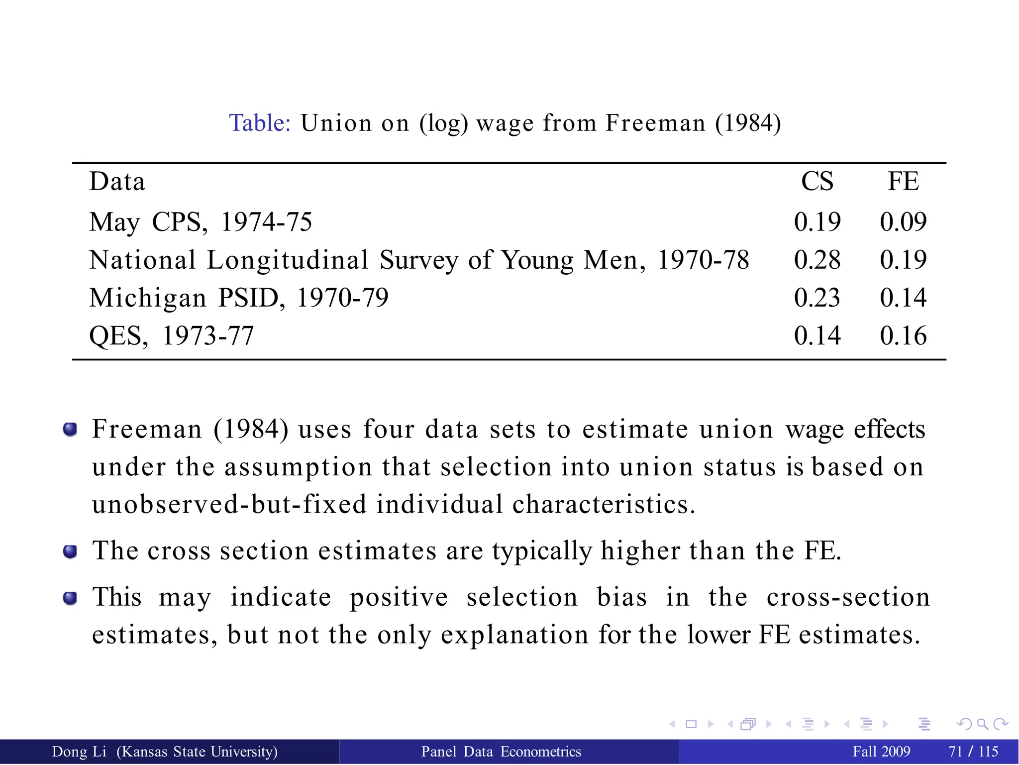
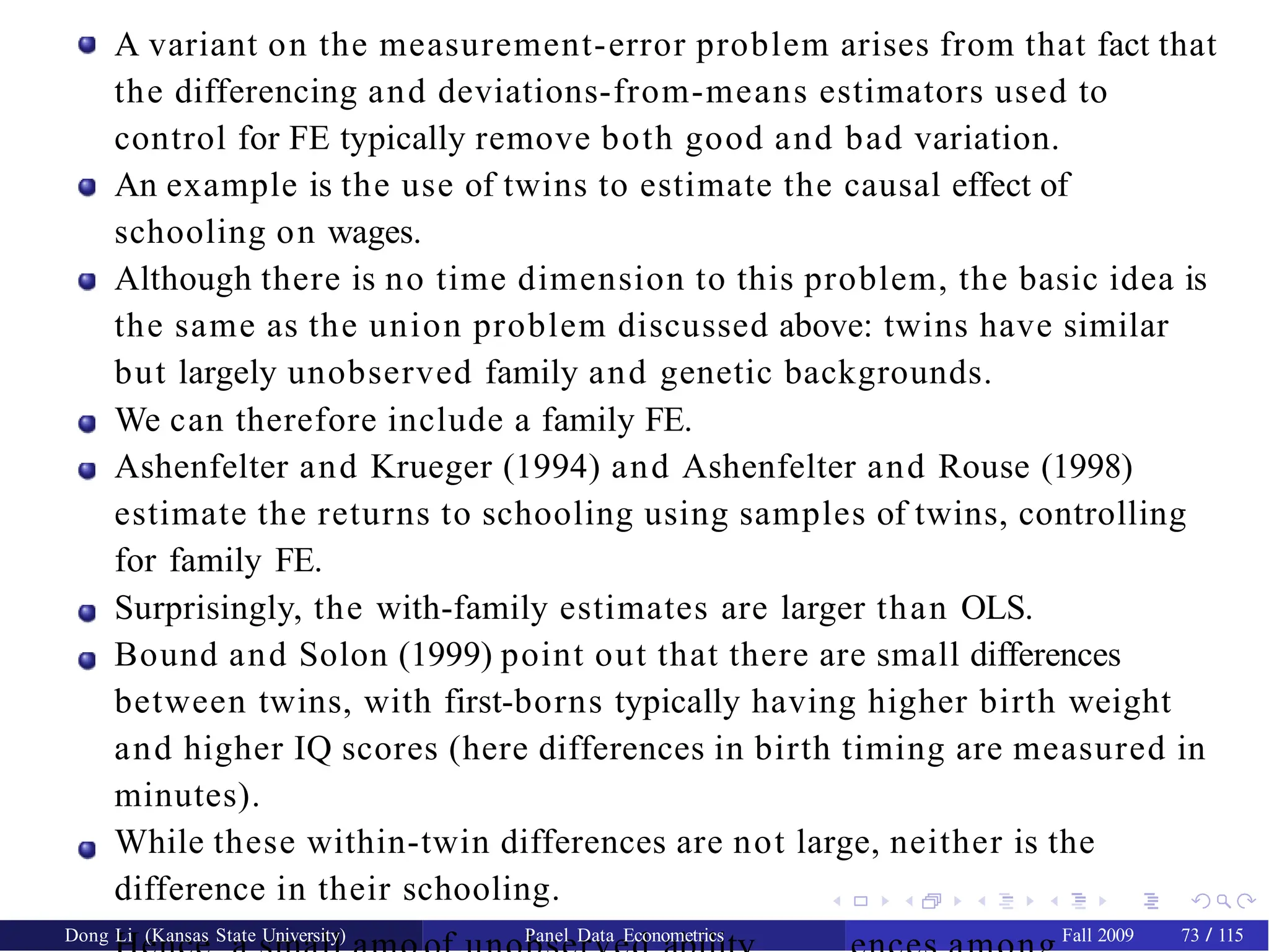


![Assuming that E(Y1ist − Y0ist |s, t) is a constant (ß ), we have:
Yist = γs + ℎt + ß Dst + гist (63)
where E(гist ) = 0.
So
E(Yist |s = PA, t = Nov) − E(Yist |s = PA, t = Feb) =
ℎNov − ℎFeb,
E(Yist |s = NJ, t = Nov) − E(Yist |s = NJ, t = Feb) = ℎN o v − ℎFeb + ß .
The population difference-in-differences,
[E(Yist |s = NJ, t = Nov) − E(Yist |s = NJ, t = Feb)]
−[E(Yist |s = PA, t = Nov) − E(Yist |s = PA, t = Feb)]
= ß ,
is the causal effect of the policy.
Dong Li (Kansas State University) Panel Data Econometrics Fall 2009 78 / 115](https://image.slidesharecdn.com/panelppt-250531033225-958aba86/75/panel-data-analysis-with-implications-and-importance-81-2048.jpg)


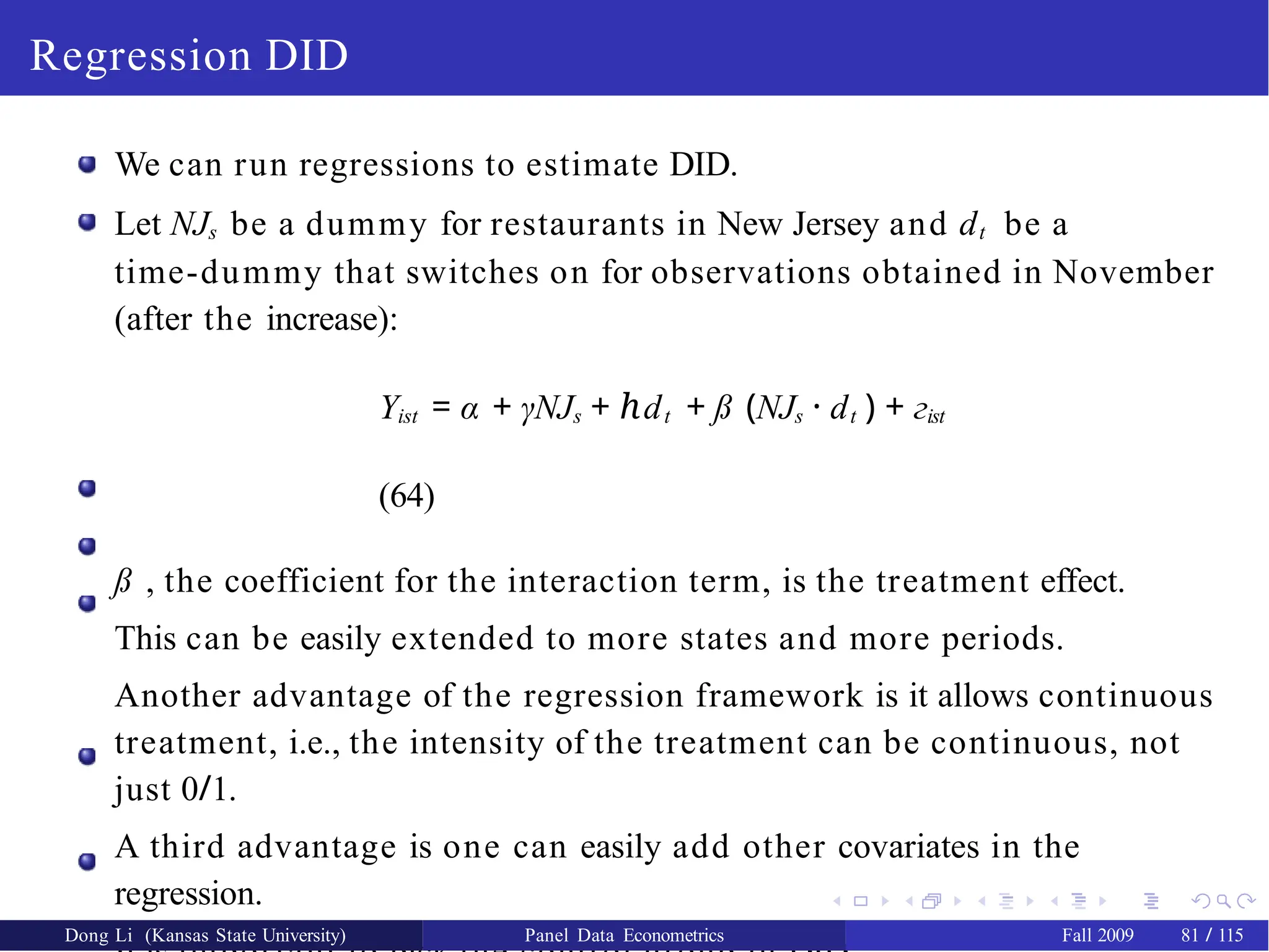
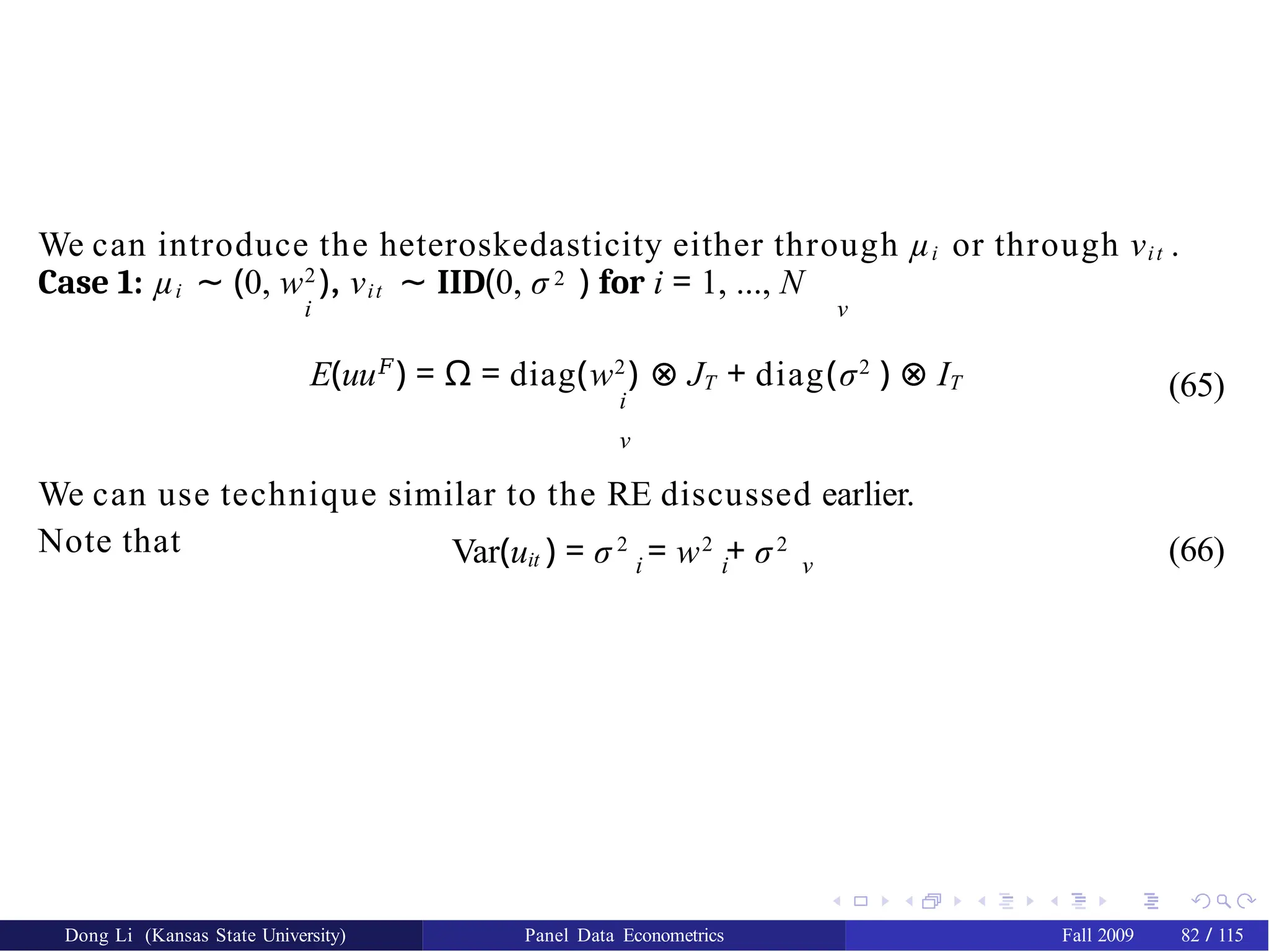
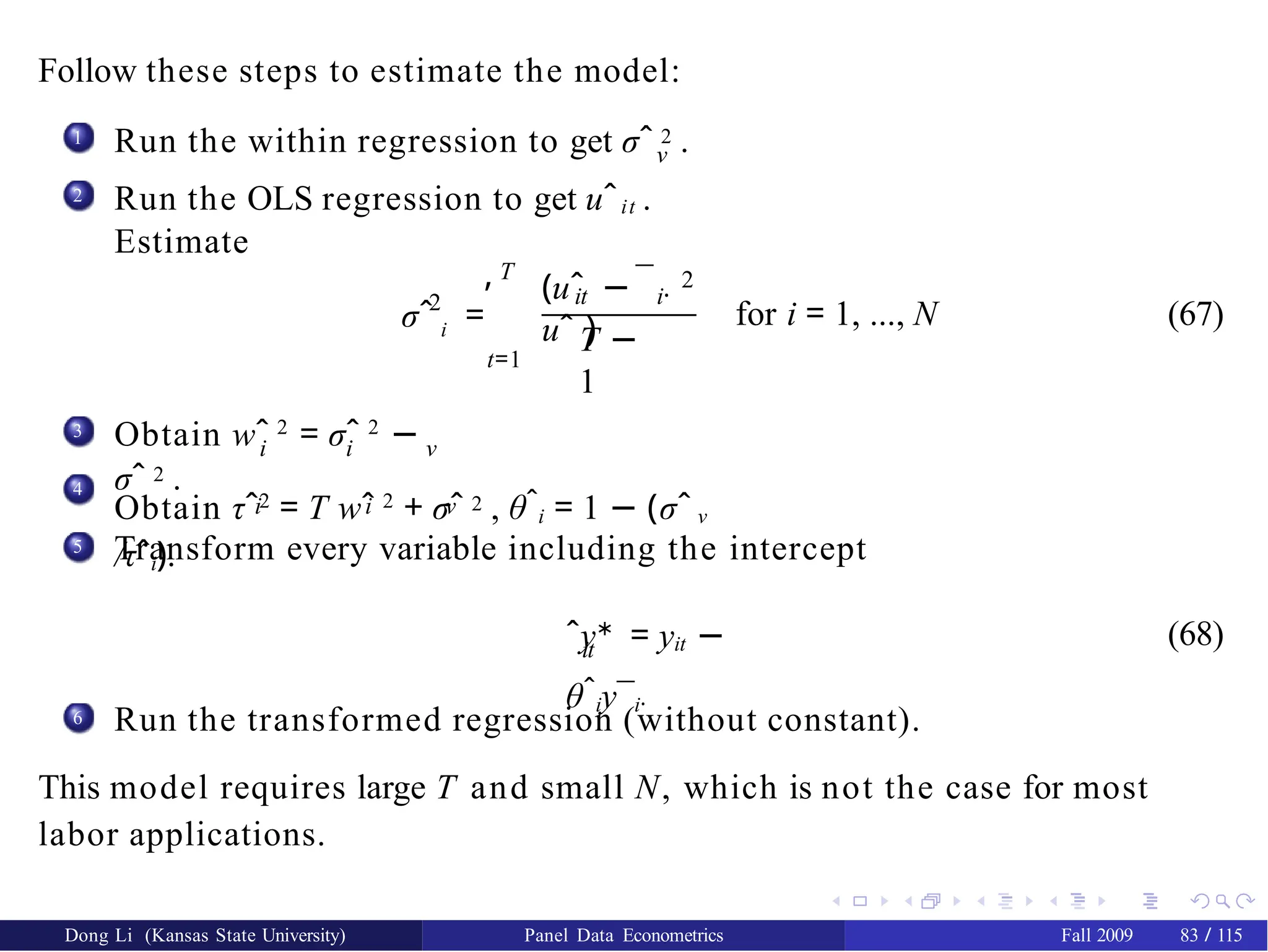
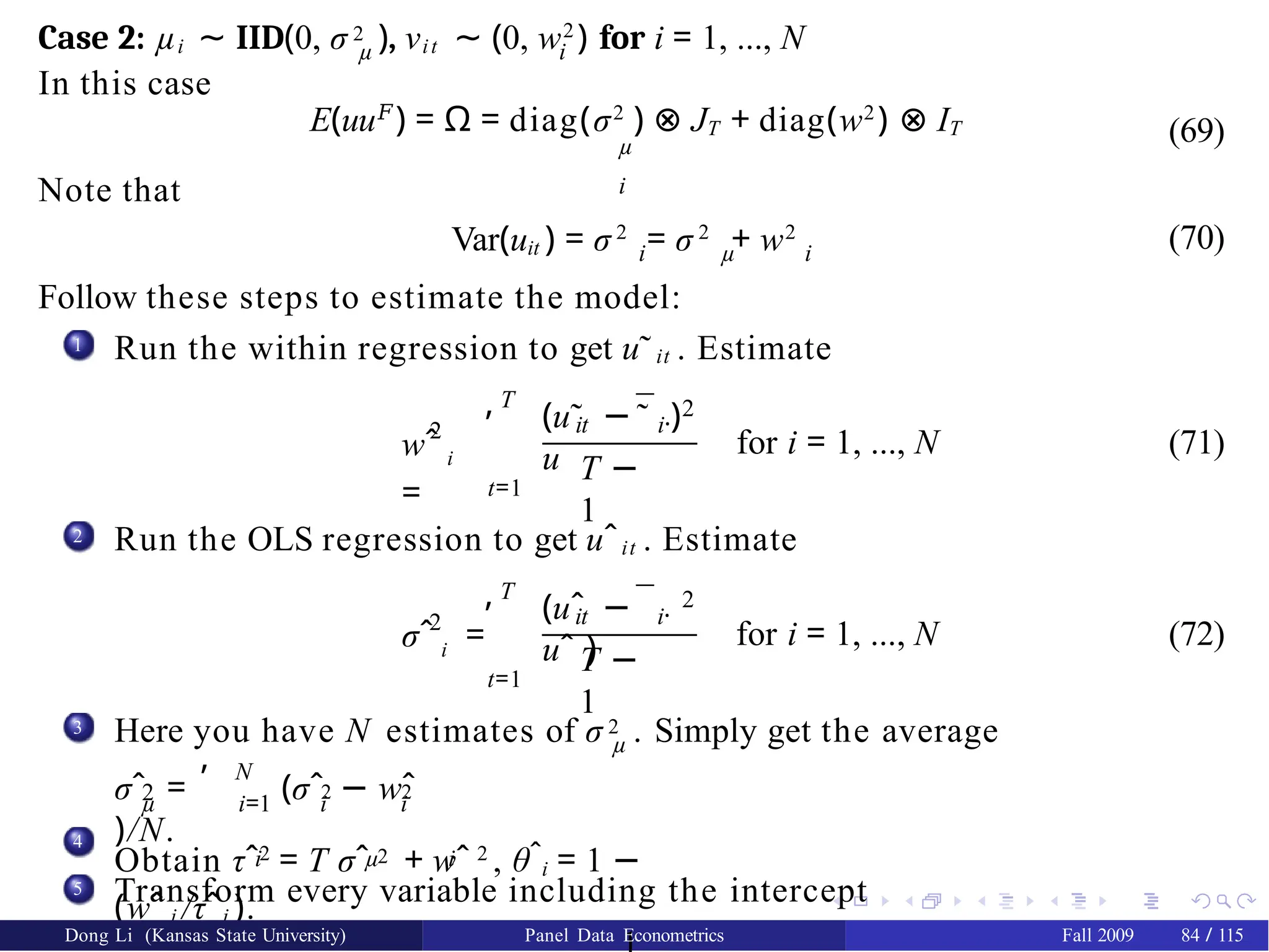
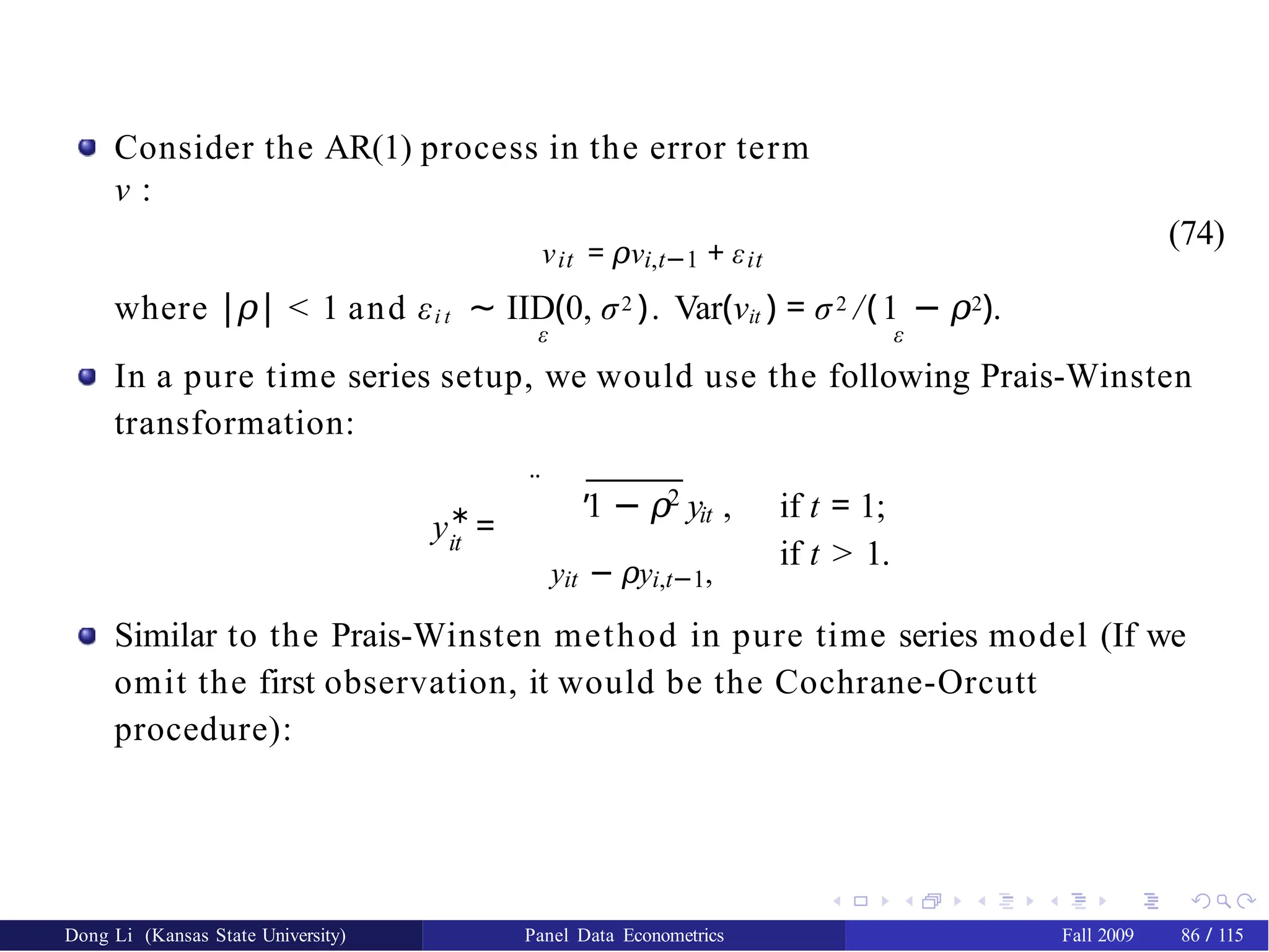
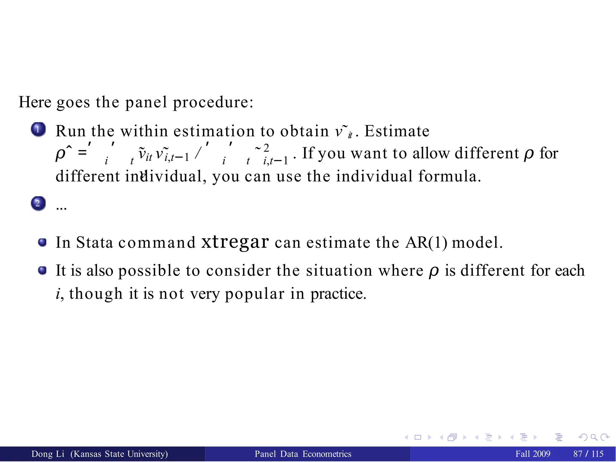
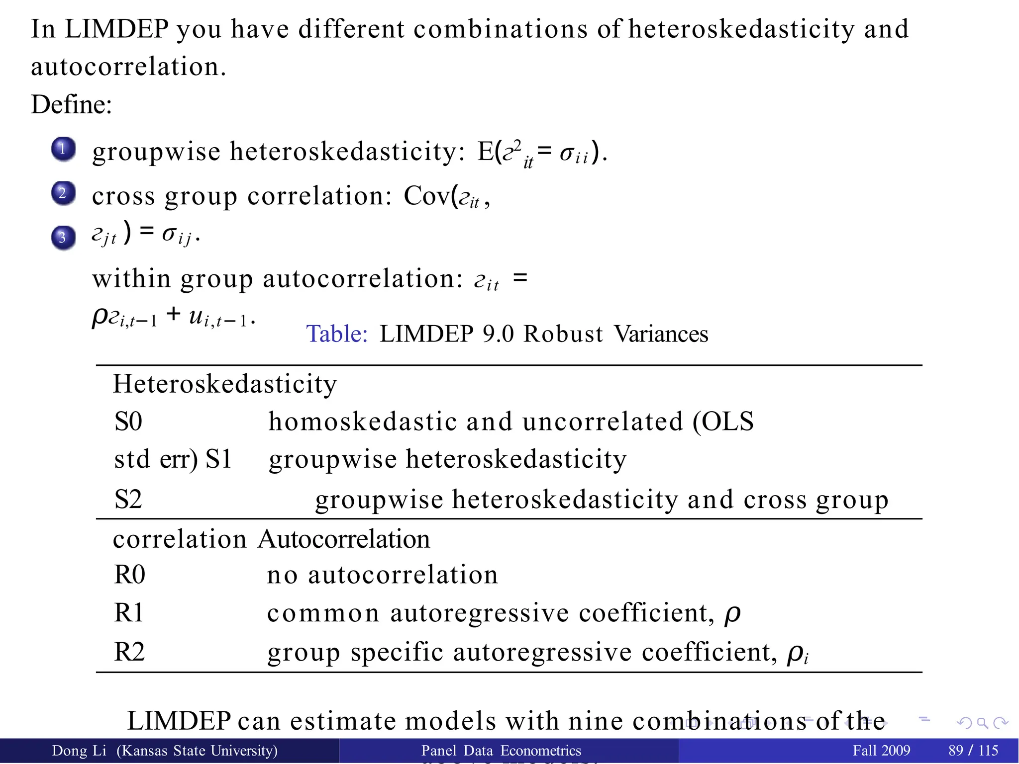
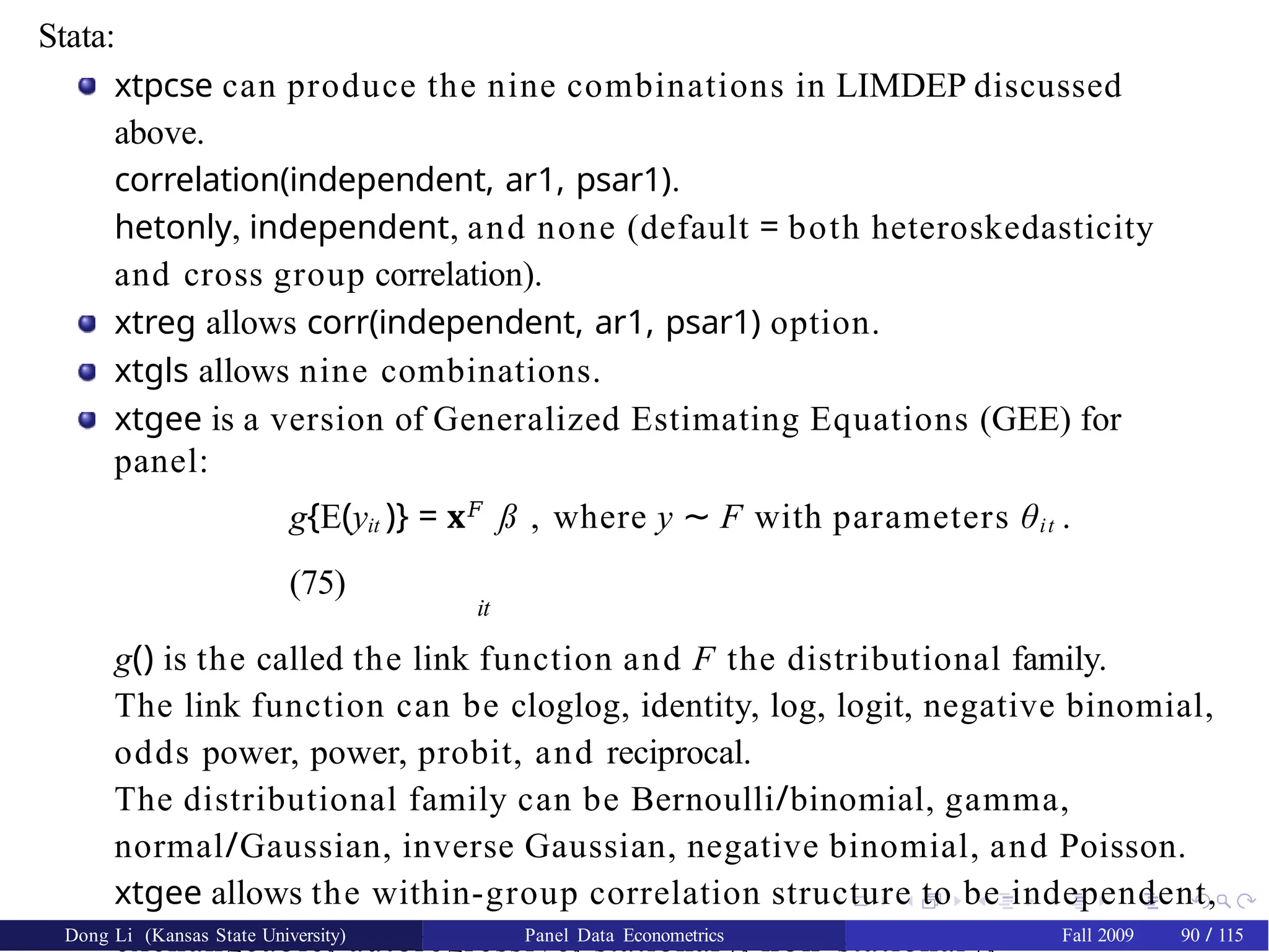
![Consider the following first structural equation of a simultaneous
equation model
y = Z δ + u (76)
where Z = [Y , X1] and δ𝐹 = (γ𝐹, ß 𝐹). As in the standard simultaneous
equation literature, Y is the set of g RHS endogenous variables, and X1
is the set of k1 included exogenous variables. Let X = [X1, X2] be the set
of all exogenous variables in the system. This equation is identified
with k2 ≥ g.
We will focus on the one-way error component model
u = Zµ µ + ν
(77)
where Zµ = (IN ⊗ ιT ) and µ𝐹 = (µ1 ,..., µN ) and ν 𝐹 = (ν11,.., νN T ) are
random vectors with zero means and covariance matrix
E
µ
ν
‚ Œ
𝐹,
𝐹
(µ ν ) =
–
2
σ IN 0
2
µ
0 σ ν INT
™
. (78)
Dong Li (Kansas State University) Panel Data Econometrics Fall 2009 93 / 115](https://image.slidesharecdn.com/panelppt-250531033225-958aba86/75/panel-data-analysis-with-implications-and-importance-96-2048.jpg)
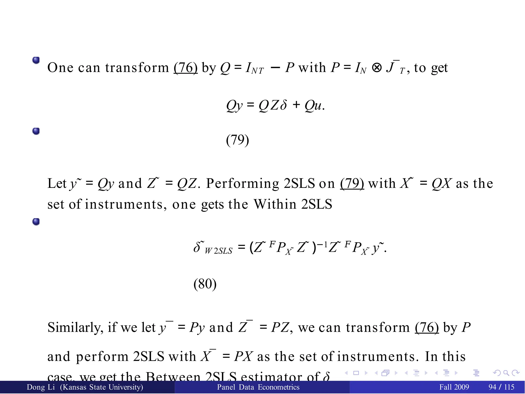
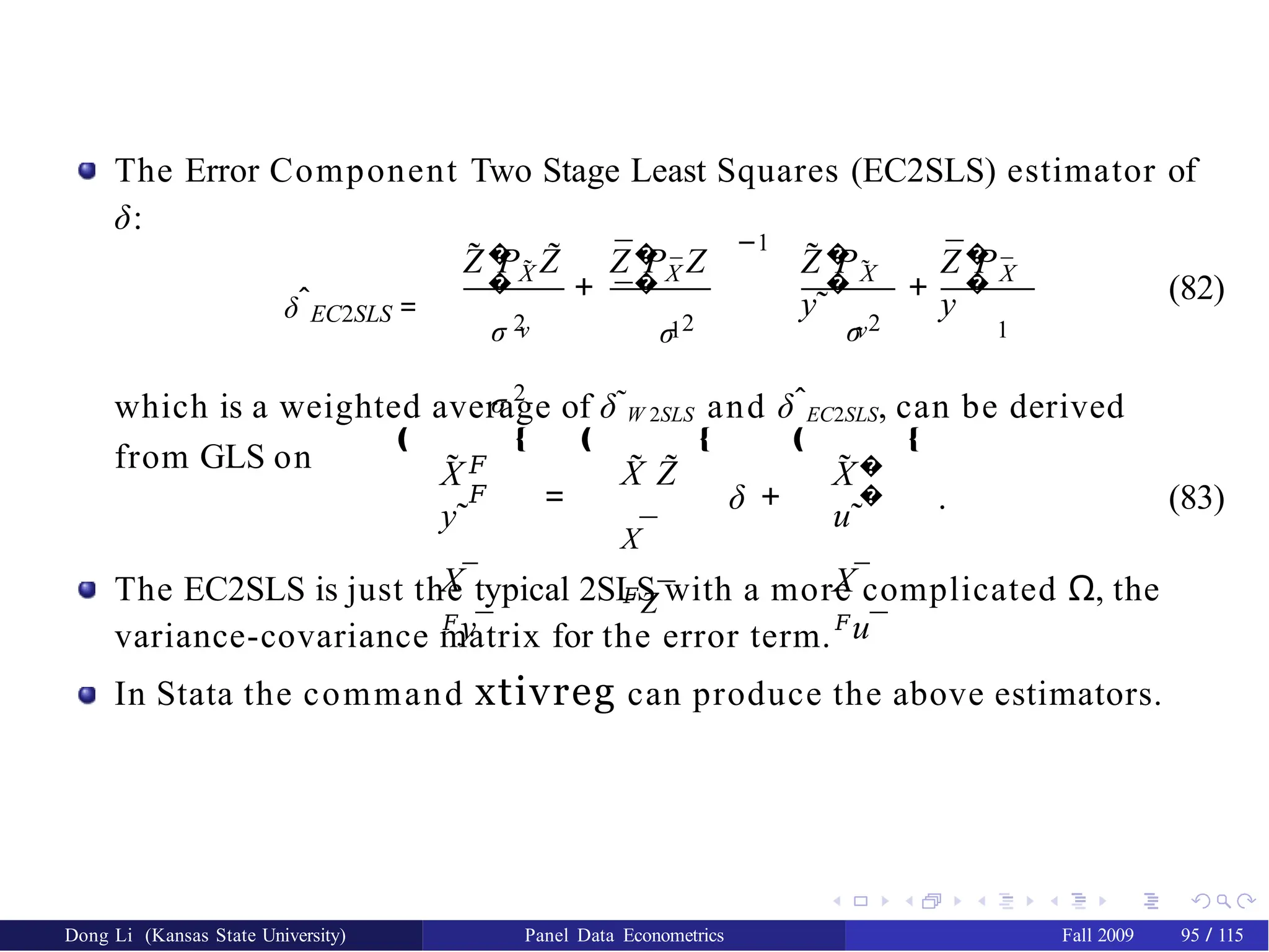

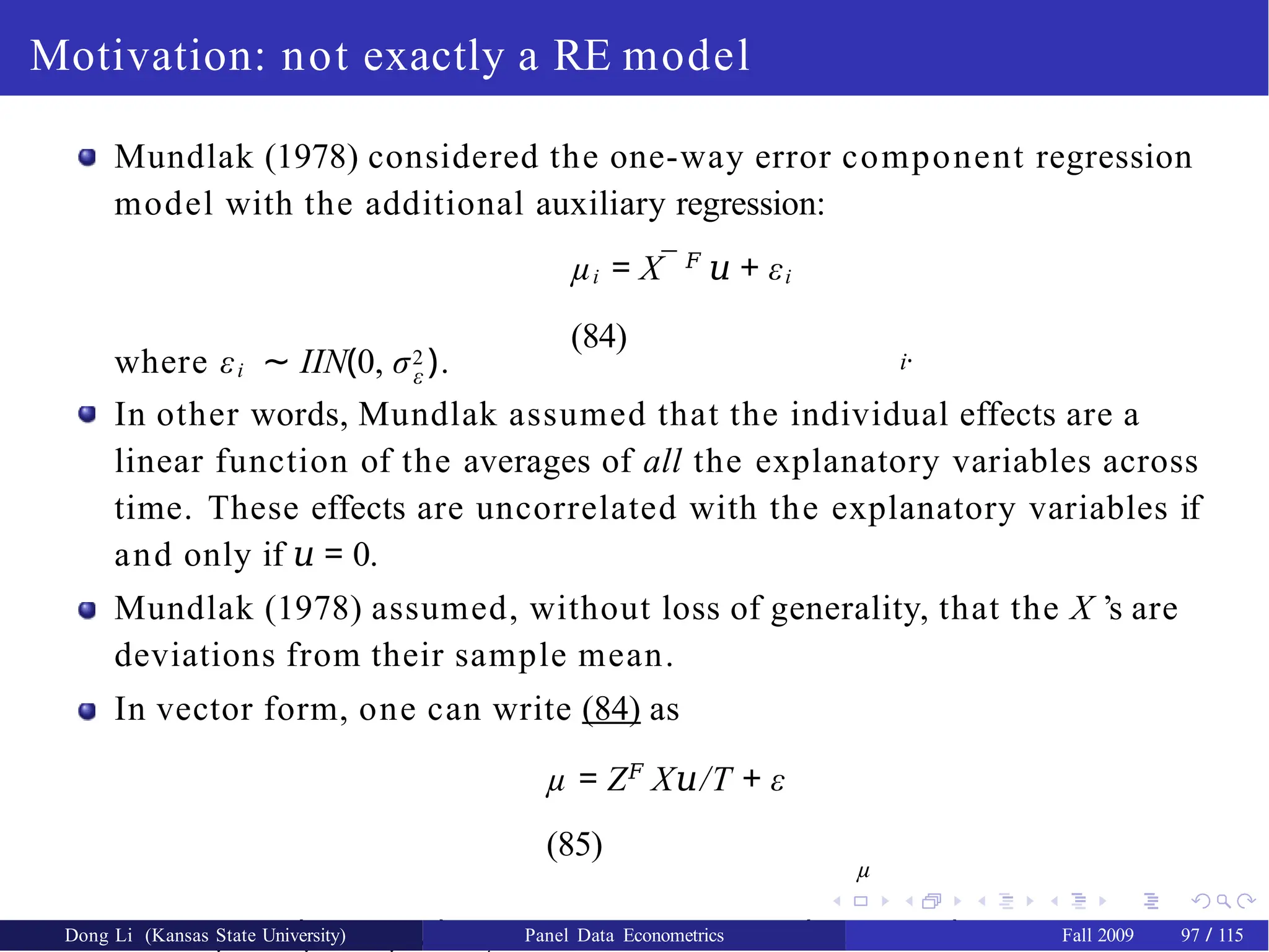
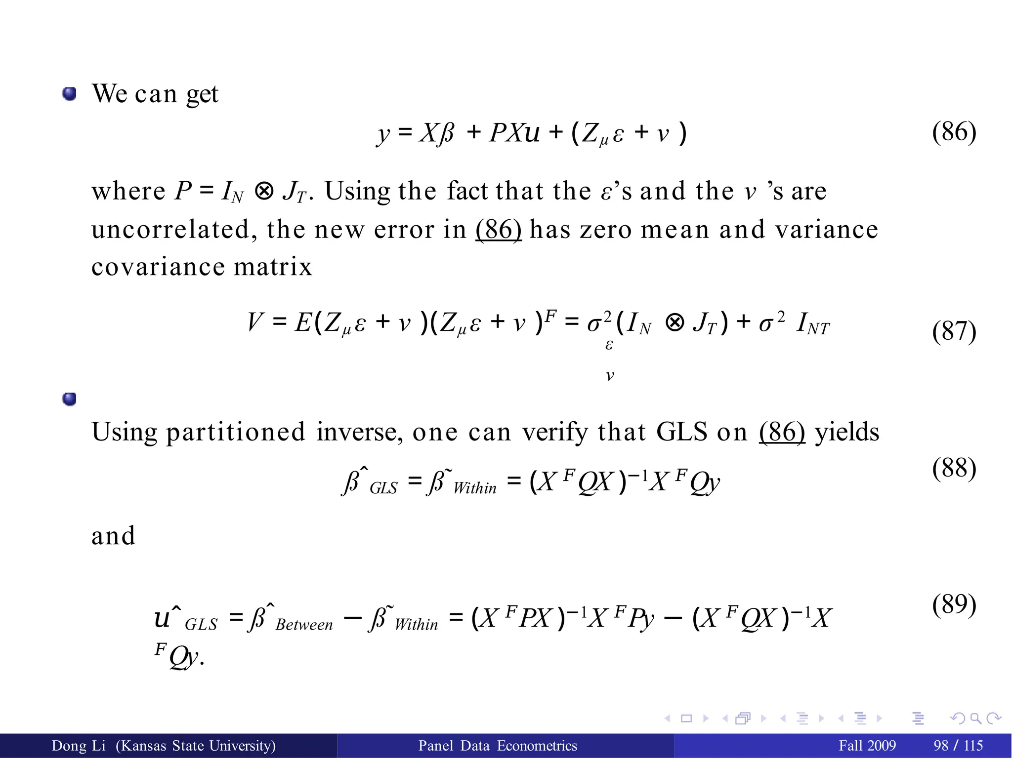
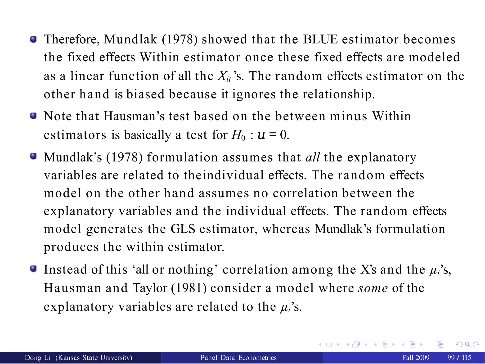
![Hausman and Taylor consider the following model:
yit = X 𝐹
ß + Z𝐹
γ + µi + νit
(90)
it i
where the Zi’s are cross-sectional time-invariant variables.
Hausman and Taylor split X and Z into two sets of variables:
X = [X1, X2] and Z = [Z1, Z2] where X1 is n × k1 , X2 is n × k2 , Z1
is n × g1,
Z2 is n × g2 and n = NT .
X1 and Z1 are assumed exogenous in the sense that they are not
correlated with µi and νit while X2 and Z2 are endogenous because
they are correlated with the µi’s, but not with the νit ’s.
The within transformation would sweep the µi’s and remove the bias,
but in the process it would also remove the Zi’s and hence the within
estimator will not give an estimate of the γ’s. To get around that,
Hausman and Taylor suggest pre-multiplying the model by Ω−1/2 and
using the following set of instruments: A0 = [Q, X1, Z1], where Q = I − P
Dong Li (Kansas State University) Panel Data Econometrics Fall 2009 100 / 115](https://image.slidesharecdn.com/panelppt-250531033225-958aba86/75/panel-data-analysis-with-implications-and-importance-103-2048.jpg)
![Breusch, Mizon, and Schmidt (1989), hereafter BMS, show that this set
of instruments yields the same projection and is therefore equivalent
to another set namely, A1 = [QX1, QX2, Z1, PX1]. The latter set of
instruments A1 is feasible, whereas A0 is not because it is NT × NT .
A1 = [QX1, QX2, Z1, PX1] are instrumental variables for [X1, X2, Z1, Z2].
Why QX2 can be instrument for X2? Because Cov(QX2, Zµ µ) = 0 though
Cov(X2, µ) /= 0.
The order condition for identification gives the result that the number
of X1’s (k1) must be at least as large as the number of Z2’s (g2). X1 is
used twice, once as averages and another time as deviations from
averages. This is an advantage of panel data allowing instruments
from within the model.
Note that the within transformation wipes out the Zi’s and does not
allow the estimation of the γ’s.
Dong Li (Kansas State University) Panel Data Econometrics Fall 2009 101 / 115](https://image.slidesharecdn.com/panelppt-250531033225-958aba86/75/panel-data-analysis-with-implications-and-importance-104-2048.jpg)
![Hausman-Taylor procedure:
1 In order to get consistent estimates of the γ’s, HT propose obtaining
the within residuals and averaging them over time
di i.
�
�
i.
ˆ ¯ ˜
= y¯ − X
ß
W (91)
2
Then, running 2SLS of dˆi on Z = [Z1, Z2] with the set of instruments
A = [Z1, X1] yields
γˆ2SLS = (Z𝐹
PAZ)−1
Z𝐹
PAdˆ
(92)
where PA = A(A𝐹A)−1A𝐹. It is clear that the order condition has to hold
(k1 ≥ g2) for (Z𝐹PAZ) to be non-singular.
Next, the variance-components estimates are obtained as follows:
3
σ
˜
2
𝐹
ν
¯X̃
= y˜ P y˜/N(T −
1
) (93)
where y˜ = Qy, X˜ = QX , P¯ A = I − PA
and
2
σ˜ 1 = (yit − Xit ߘW − Ziγˆ2SLS)𝐹P(yit − Xit ߘW − Ziγˆ2SLS)
N
(94)
This last estimate is based upon an NT vector of residuals.
Dong Li (Kansas State University) Panel Data Econometrics Fall 2009 101 / 115](https://image.slidesharecdn.com/panelppt-250531033225-958aba86/75/panel-data-analysis-with-implications-and-importance-105-2048.jpg)
![4 Once the variance components estimates are obtained, the model is
ˆ −1
2
transformed using Ω as follows:
Ω
^
− 1
2 ^− 1
2 ^− 1
2 ^
y = Ω Xß + Ω Zγ +
Ω
− 1
2 u
(95)
The HT estimator is basically 2SLS on the above regression using
AHT = [X˜1 , X˜2, Z1, X¯1] as a set of instruments.
Comments:
1
If k1 < g2, then the equation is under-identified. In this case ߈HT = ߘW
and γˆHT does not exist.
2
If k1 = g2, then the equation is just-identified. In this case, ߈HT = ߘW
and γˆHT = γˆ2SLS given by (92).
3 If k1 > g2, then the equation is over identified and the HT estimator
obtained from (95) is more efficient than the within estimator.
Dong Li (Kansas State University) Panel Data Econometrics Fall 2009 102 / 115](https://image.slidesharecdn.com/panelppt-250531033225-958aba86/75/panel-data-analysis-with-implications-and-importance-106-2048.jpg)
![Amemiya and MaCurdy (1986), hereafter AM, suggest a more efficient
1 1 1
set of instruments A2 = [QX1, QX2, X ∗
, Z1] where X ∗
= X 0
⊗ ιT
and
0
1
X =
X11 X12
..
X1T
. . .
. . ..
.
XN1 XN2
..
XNT
(96)
is an N × k1 T matrix.
So X1 is used (T + 1) times, once as X1 and T times as X ∗
.
1
The order condition for identification is now more likely to be satisfied
(Tk1 > g2).
However, this set of instruments require a stronger exogeneity
assumption than that of Hausman and Taylor (1981).
The latter requires only uncorrelatedness of the mean of X1 from the
µi’s, while Amemiya and MaCurdy (1986) require uncorrelatedness at
each point in time.
Breusch, Mizon, and Schmidt (1989) suggest yet a more efficient set of
instruments A3 = [QX1, QX2, PX1,(QX1)∗,(QX2)∗, Z1].
Dong Li (Kansas State University) Panel Data Econometrics Fall 2009 102 / 115](https://image.slidesharecdn.com/panelppt-250531033225-958aba86/75/panel-data-analysis-with-implications-and-importance-107-2048.jpg)
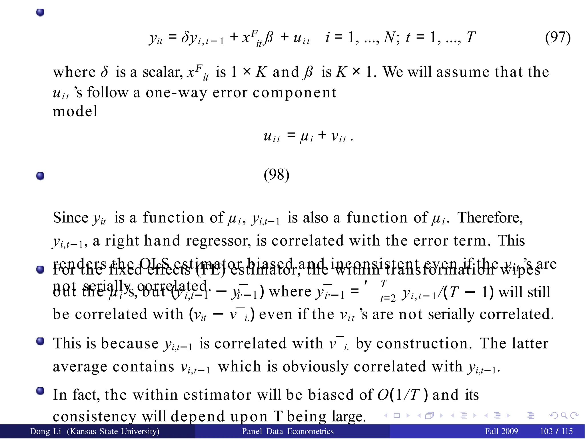
![where ∆νi = (νi3 − νi 2 ,..., νiT − νi,T −1) and
G =
2 −1 0 . . . 0 0
−1
.
2
.
−1 . . . 0
. ... .
0
.
.
0
.
0
. .
0 . . . 2
.
−
1
0 0 0 . . .
−1
2
is (T − 2) × (T − 2), since ∆ν is MA(1) with unit
root. Define
[yi1]
0
i
W =
i1 i2
[y , y ]
...
0 [y , ...,
y
i1 i,T
−2
]
(104)
1 N
Then, the matrix of instruments is W = [W 𝐹
, ..., W 𝐹
]𝐹 and the
moment
equations described above are given by E(W 𝐹
∆νi) = 0.
i
Pre-multiplying the differenced equation (100) in vector form by W 𝐹,
one gets
W 𝐹
∆y = W 𝐹
(∆y−1)δ + W 𝐹
∆ν
(105)
Dong Li (Kansas State University) Panel Data Econometrics Fall 2009 104 / 115](https://image.slidesharecdn.com/panelppt-250531033225-958aba86/75/panel-data-analysis-with-implications-and-importance-114-2048.jpg)
![Performing GLS on the above regression one gets the Arellano and
Bond (1991) one-step consistent estimator
δˆ1
= [(∆y−1)𝐹
W (W 𝐹
(IN ⊗ G)W )−1
W 𝐹
(∆y−1)]−1
[(∆y−1)𝐹
W (W 𝐹
(IN ⊗ G)W )−1
W 𝐹
(∆y)]
(106)
The optimal Generalized Method of Moments (GMM) estimator of δ1
(Hansen, 1982) for N → ∞ and T fixed using only the above moment
restrictions yields the same expression except that
W 𝐹(IN ⊗ G)W = ΣN
W 𝐹
GWi is replaced by VN = ΣN
W 𝐹
(∆ν )
(∆ν )𝐹Wi.
i=1 i
i=1 i
This GMM estimator requires no knowledge concerning the initial
conditions or the distributions of νi and µi.
To make this estimator feasible, ∆ν is replaced by differenced
residuals obtained from the preliminary consistent estimator δˆ1.
The resulting estimator is the two-step Arellano and Bond (1991)
GMM estimator:
δˆ2
= [(∆y−1)𝐹
W Vˆ −1
W 𝐹
(∆y−1)]−1
[(∆y−1)𝐹
W Vˆ −1
W 𝐹
(
∆ y)] (107)
N N
Dong Li (Kansas State University) Panel Data Econometrics Fall 2009 104 / 115](https://image.slidesharecdn.com/panelppt-250531033225-958aba86/75/panel-data-analysis-with-implications-and-importance-115-2048.jpg)
![A consistent estimate of asymptotic Var(δˆ2) is given by the first term in
the above equation,
ˆ
V̂ar(δ ) = [(∆
2 −1 N
𝐹 ˆ−1
𝐹
y ) WV W (∆ −1
y )]−1
(108)
Note that δˆ1 and δˆ2 are asymptotically equivalent if the νit ’s are
IID(0, σ 2 ).
ν
What if we have exogenous variables?
If there are additional strictly exogenous regressors xit ’s with
E(xitνis) = 0 for all t, s = 1, 2, ..., T , but where all the xit ’s are correlated
with µi , then all the xit ’s are valid instruments for the first differenced
i1 i2 iT
equation. Therefore, [x𝐹
, x𝐹
, ..., x𝐹
] should be added to each
diagonal
element of Wi in (104):
i
W =
i1
𝐹
𝐹
i1 i2
�
�
iT
[y , x , x , ...,
x ]
0
i1 i2 iT
[yi1, yi2, x𝐹
, x𝐹
, ...,
x𝐹
] ...
0 [yi1, ..., yi,T −2, x𝐹
,
x𝐹
i1 i
(109)
Dong Li (Kansas State University) Panel Data Econometrics Fall 2009 104 / 115](https://image.slidesharecdn.com/panelppt-250531033225-958aba86/75/panel-data-analysis-with-implications-and-importance-116-2048.jpg)
![In this case, (105) becomes
W 𝐹
∆y = W 𝐹
(∆y−1)δ + W 𝐹
(∆X )ß + W 𝐹
∆ν
(110)
where ∆X is the stacked N(T − 2) × K matrix of observations on ∆xit .
One-step and two-step estimators of (δ, ß 𝐹) can be obtained from
δ̂
߈
‚ Œ
−1 −1 −1
N N
= ([∆y ∆X ]𝐹
W Vˆ −1
W 𝐹
[∆y ∆X ])−1
([∆y ∆X ]𝐹
W Vˆ −1
W
𝐹
∆y). (111)
If xit ’s are predetermined rather than strictly exogenous with E(xitνis) /= 0
for s > t, and zero otherwise, then only [x𝐹
, x𝐹
, ..., xi,(s−1)] are
valid
i1 i2
instruments for the differenced equation at period s. This can be
illustrated as follows: For t = 3, the first differenced equation becomes
i3 i2
yi3 − yi2 = δ(yi2 − yi1) + (x𝐹
− x𝐹
)ß + (νi3 − νi2) (112)
i1 i2
For this equation, x𝐹
and x𝐹
are valid instruments, since both are
not
correlated with (νi 3 − νi2). For t = 4, the next period we observe this
relationship
yi4 − yi3 = δ(yi3 − yi2) + (x𝐹
− x𝐹
)ß + (νi4 − νi3)
Dong Li (Kansas State University) Panel Data Econometrics Fall 2009 104 / 115](https://image.slidesharecdn.com/panelppt-250531033225-958aba86/75/panel-data-analysis-with-implications-and-importance-117-2048.jpg)
![i1 i2 i3
and we have additional instruments since now x𝐹
, x𝐹
and x𝐹
are
not
correlated with (νi4 − νi3). Continuing in this fashion, we get
i
W =
i1
�
�
�
�
i1 i2
[y , x ,
x ]
0
i1 i2 i3
[yi1, yi2, x𝐹
, x𝐹
,
x𝐹
] ...
0 i1 i,T
−1
[yi1, ..., yi,T −2, x𝐹
, ..., x𝐹
]
and one and two-step estimators are again given by (110) with this
choice of Wi.
There are further extensions to this model, mainly with additional
moment conditions. Such as the system Arellano-Bover and
Blundell-Bond estimators.
In Stata and LIMDEP, the dynamic panel data models are available.
xtabond, xtdpd, and xtdpdsys in Stata.
Dong Li (Kansas State University) Panel Data Econometrics Fall 2009 105 / 115](https://image.slidesharecdn.com/panelppt-250531033225-958aba86/75/panel-data-analysis-with-implications-and-importance-118-2048.jpg)


![[DSC Europe 25] Jim Sterne - Adopting Generative AI Capabilities Into the Ent...](https://cdn.slidesharecdn.com/ss_thumbnails/sxhpofuorcagxsaulkmt-3-251204082258-7e66bc48-thumbnail.jpg?width=640&height=640&fit=bounds)
![[DSC Europe 25] Dusan Jovicic - AI Story: From on-prem to cloud and back agai...](https://cdn.slidesharecdn.com/ss_thumbnails/8kp49m6uq22ifnbwhfnk-2-251205085715-964d11a6-thumbnail.jpg?width=640&height=640&fit=bounds)
![[DSC Europe 25] Goran Obradovic - The Rise of Sovereign AI: Building the Regi...](https://cdn.slidesharecdn.com/ss_thumbnails/7nw2xxixrxqdxvrb5wca-6-251205085714-ab09a2ac-thumbnail.jpg?width=640&height=640&fit=bounds)


![[DSC Europe 25] Petar Zivanov - AI meets documents From chatbots to AI-powere...](https://cdn.slidesharecdn.com/ss_thumbnails/xer2bb6nrdc8pdpev0pc-8-251204082258-7c2fa4a1-thumbnail.jpg?width=640&height=640&fit=bounds)

![[DSC Europe 25] Andy Cotgreave - Nothing is new in analytics.pptx](https://cdn.slidesharecdn.com/ss_thumbnails/mba4vzcurvoh5lfrd5zw-6-251205194645-341bbbbe-thumbnail.jpg?width=640&height=640&fit=bounds)
