Download to read offline

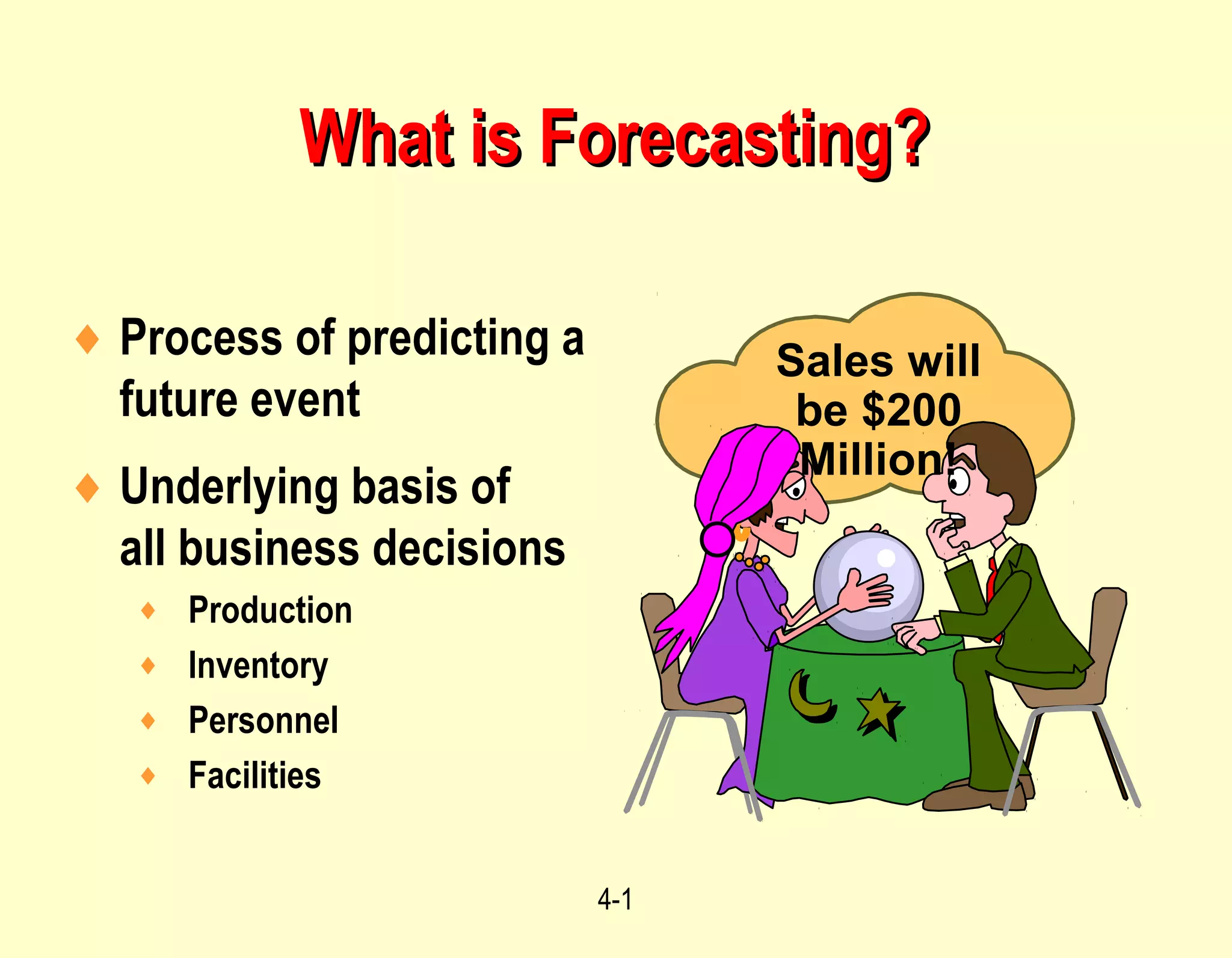
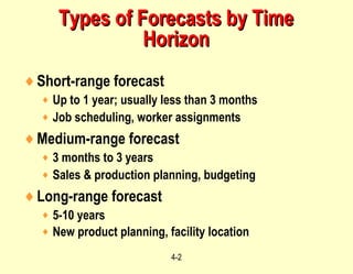
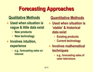
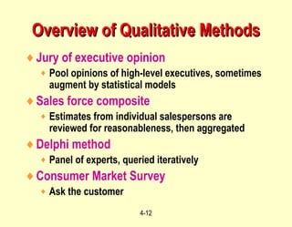
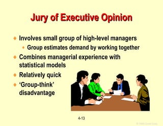
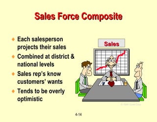
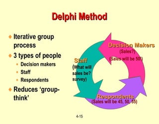
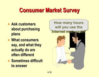
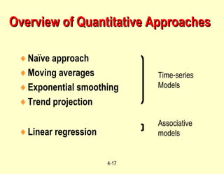
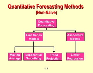
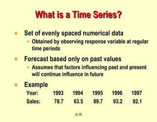
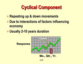
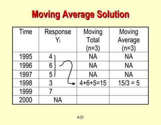
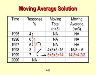
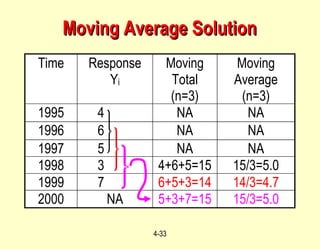
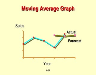
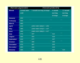
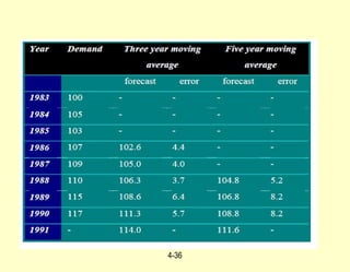
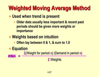
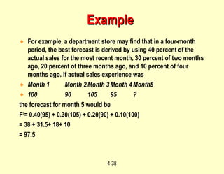

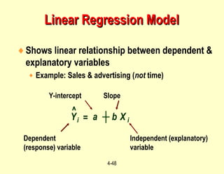
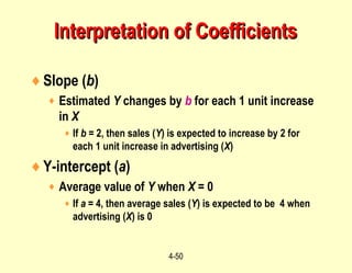
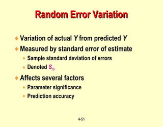
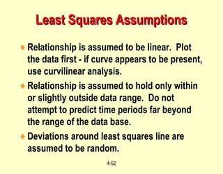

This document discusses various forecasting techniques used to predict future events and trends. It describes short, medium, and long-range forecasts used for production planning, budgeting, and new product development. Both qualitative methods like executive opinion and surveys, and quantitative methods like time series analysis, moving averages, and regression are covered. The key factors influencing forecasts like product life cycles and demand trends are also explained.


![Product1 [3] forecasting v2](https://cdn.slidesharecdn.com/ss_thumbnails/product13-forecastingv2-190226041012-thumbnail.jpg?width=640&height=640&fit=bounds)