This document outlines key concepts related to forecasting, including:
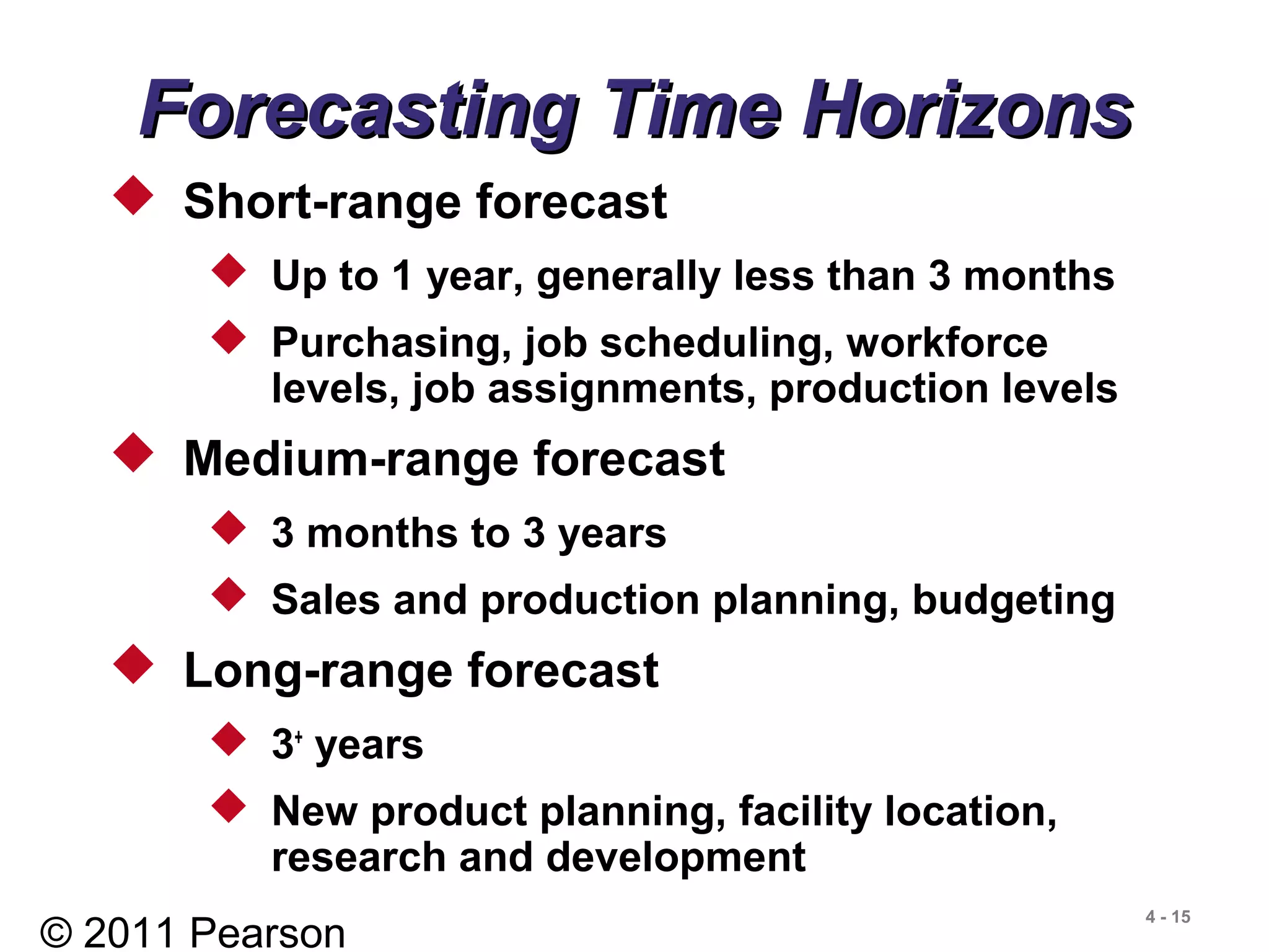
- The three time horizons for forecasting: short, medium, and long range.
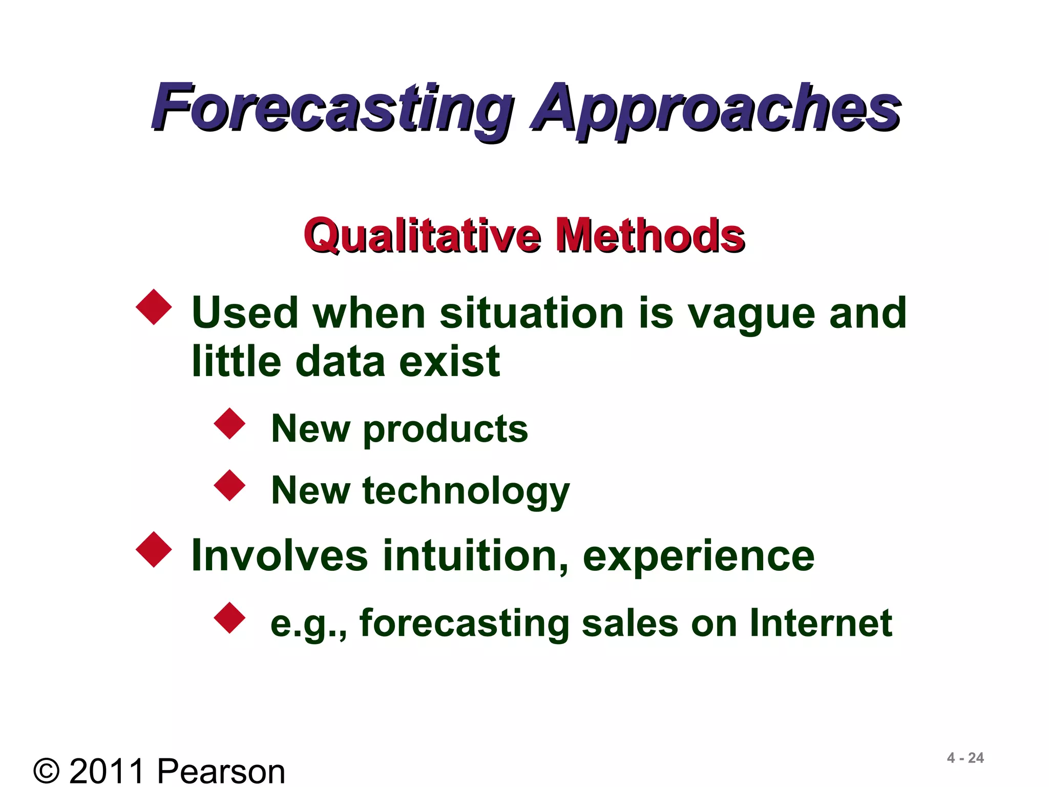
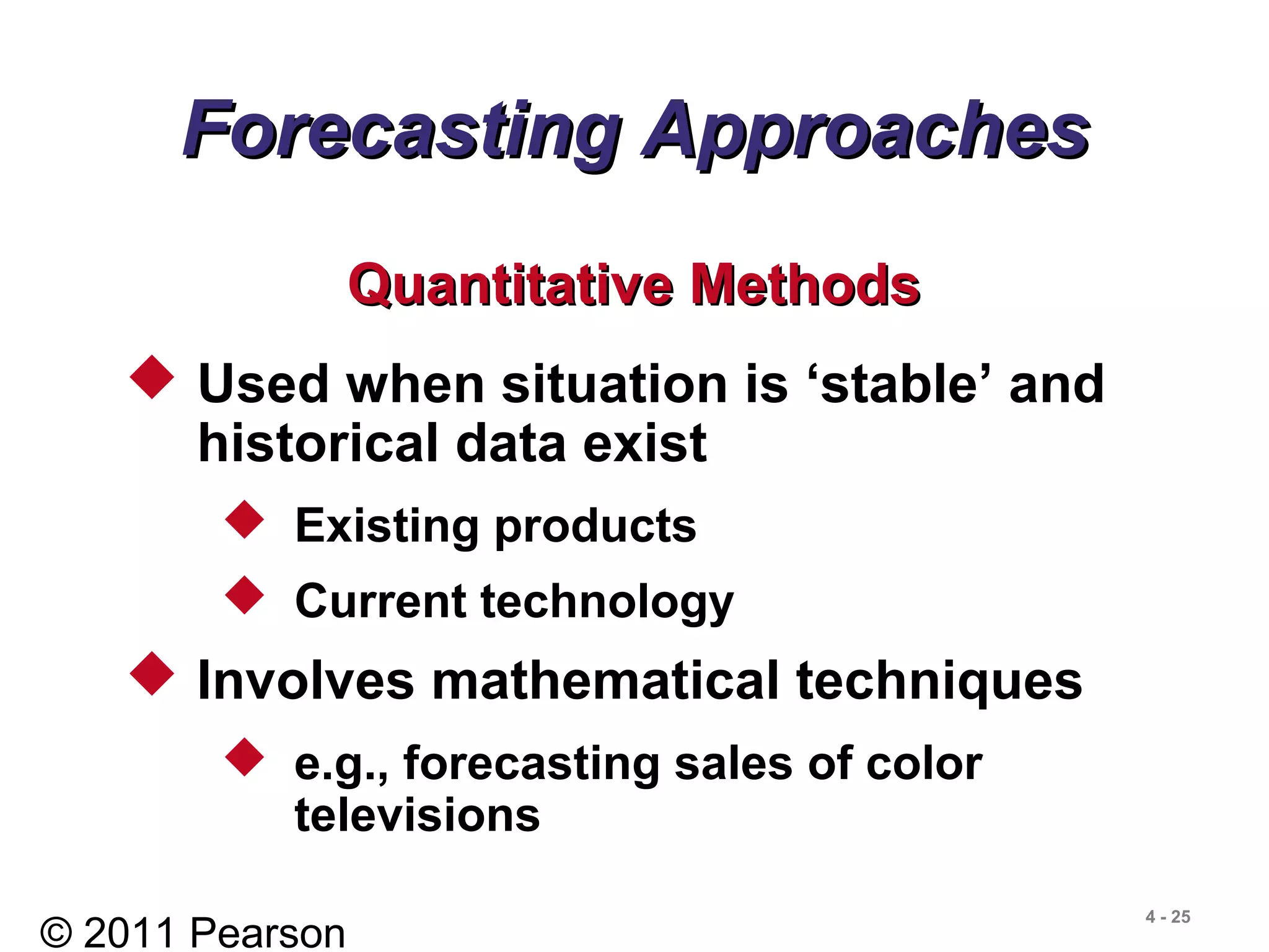
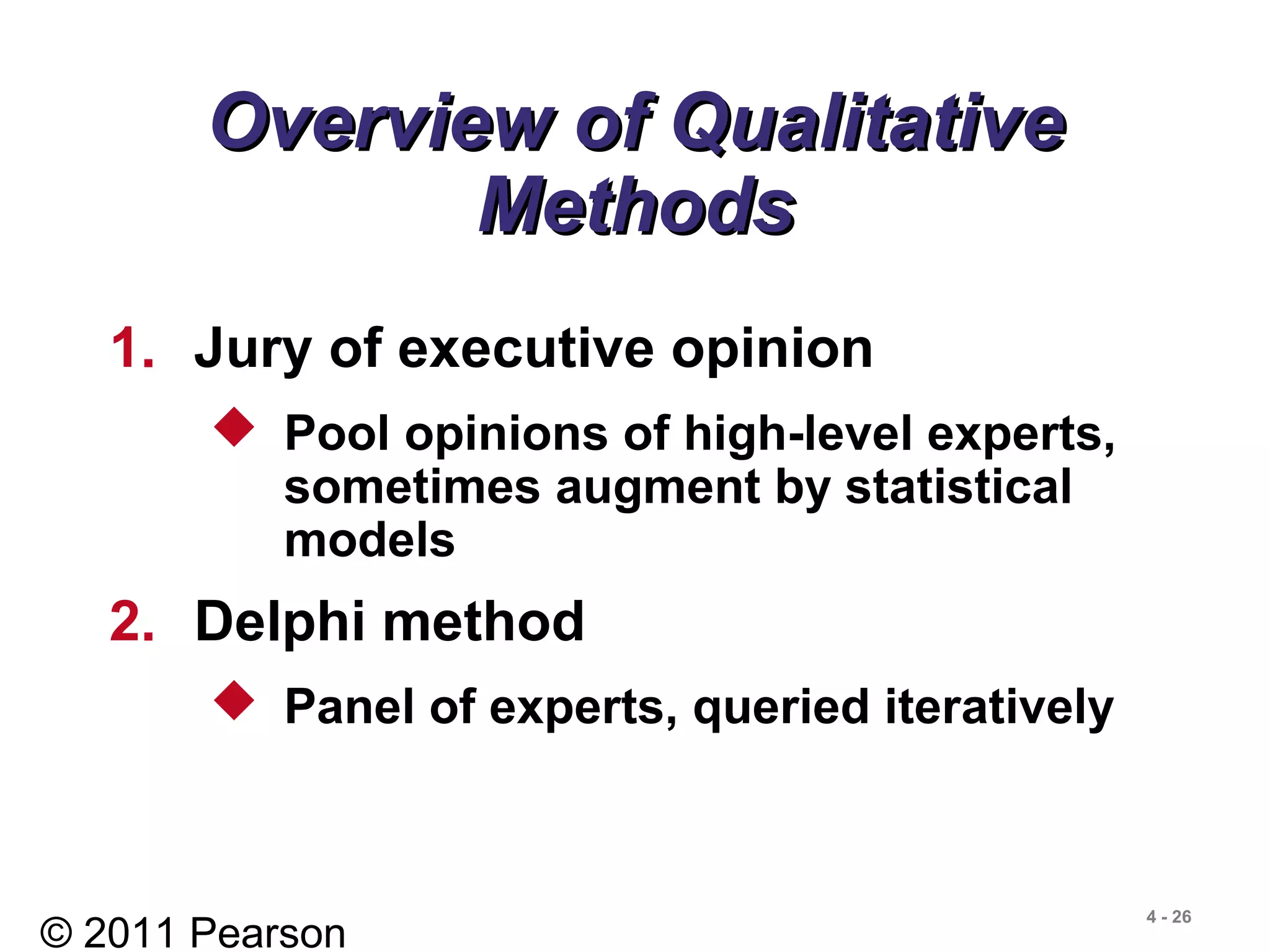
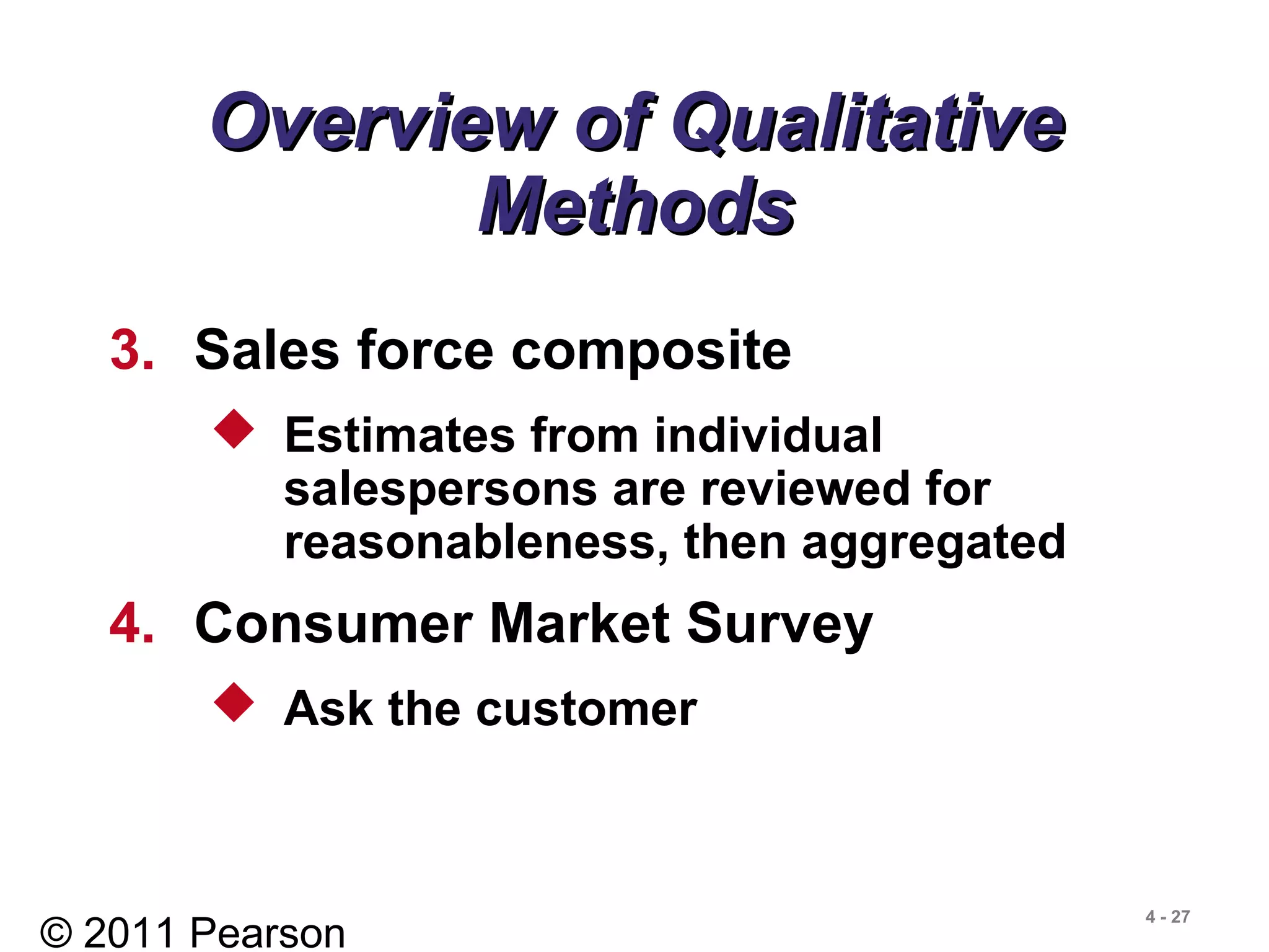
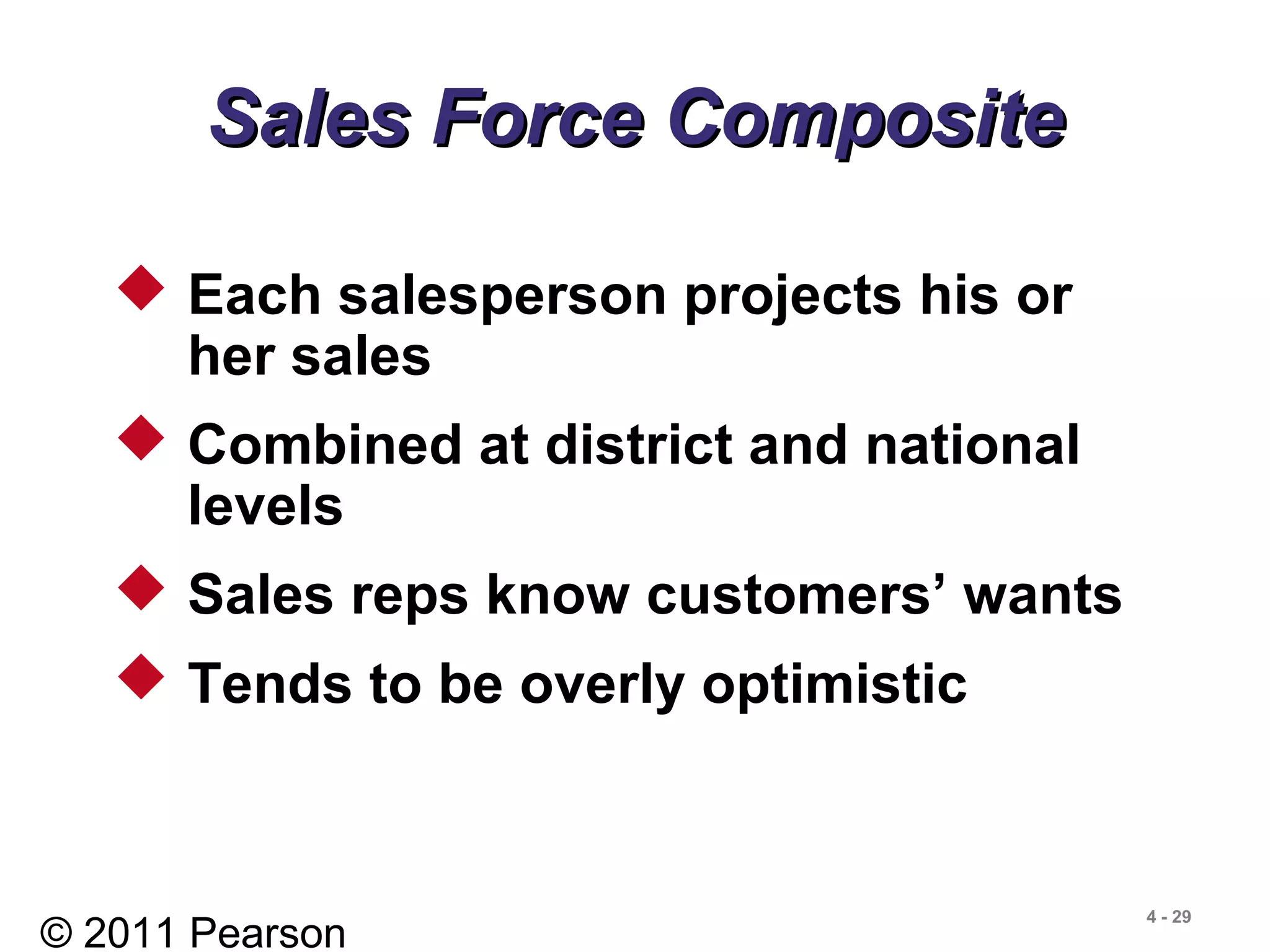
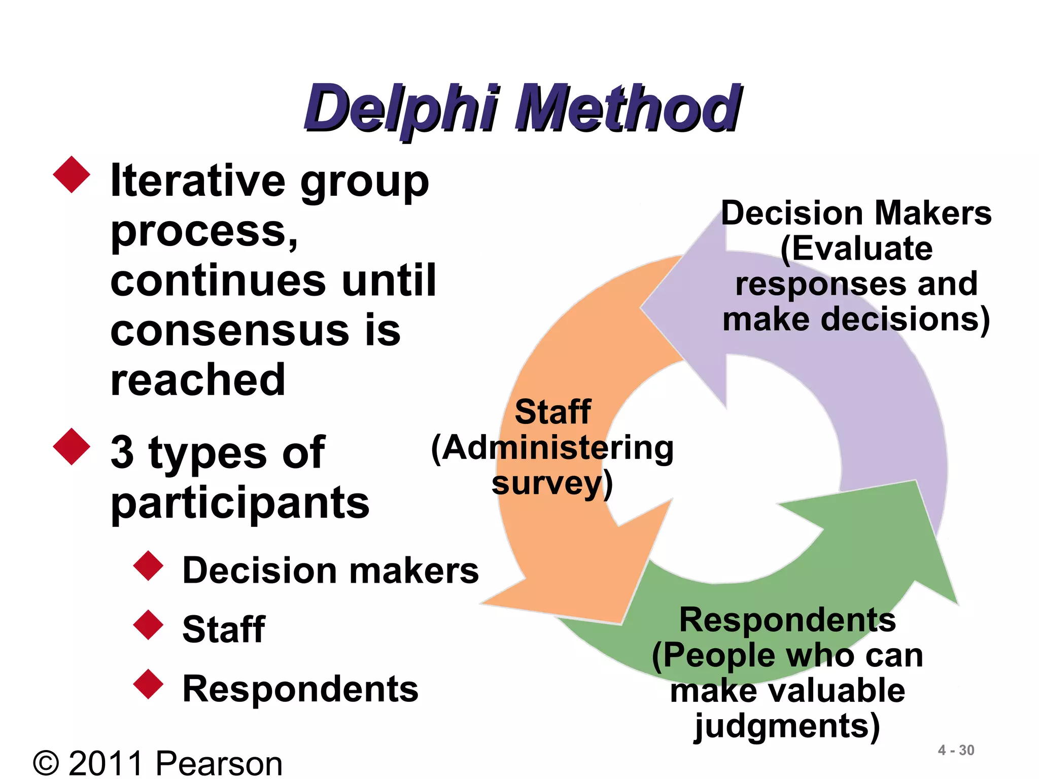
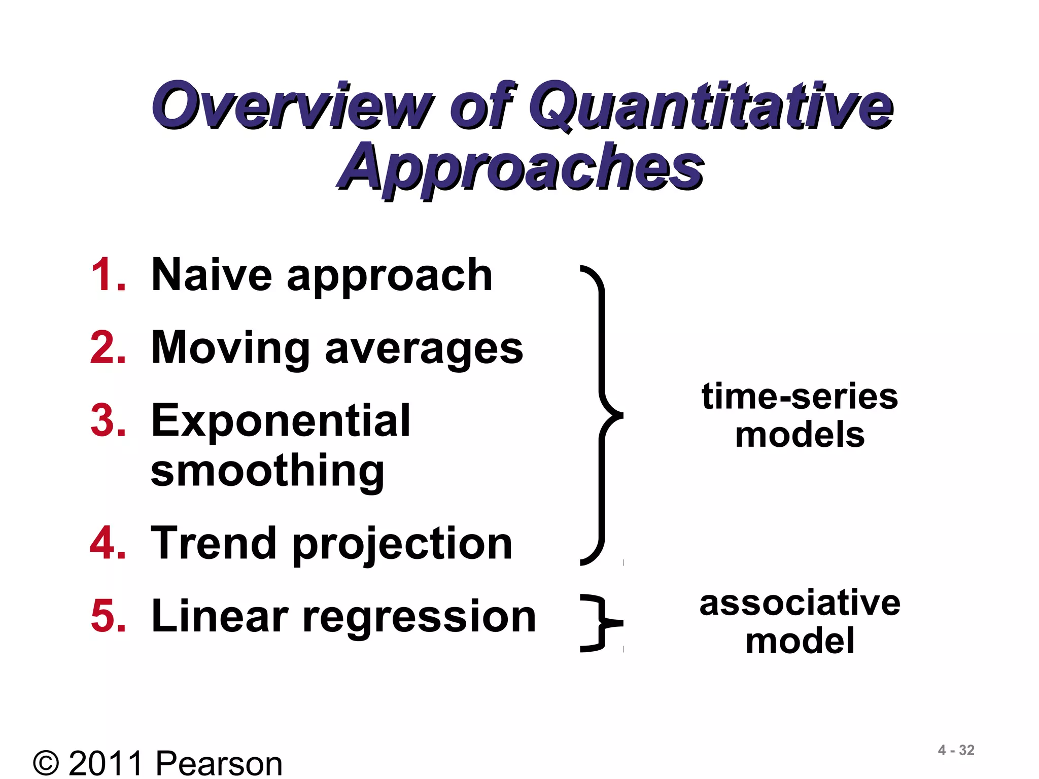
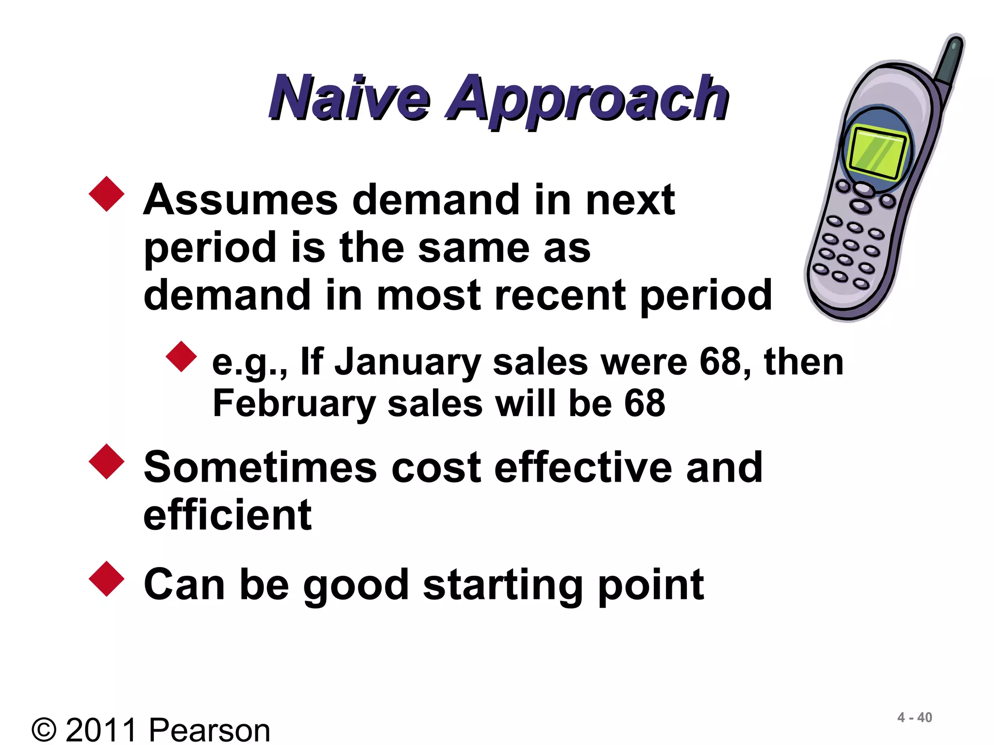
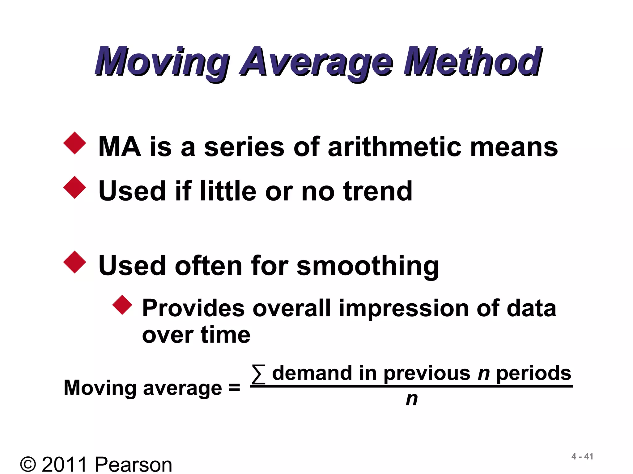
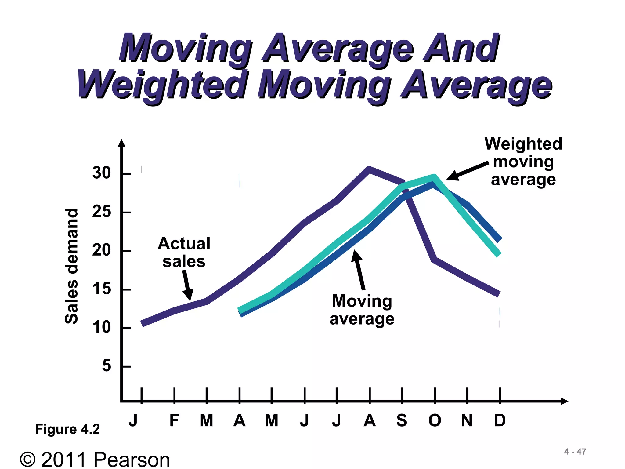
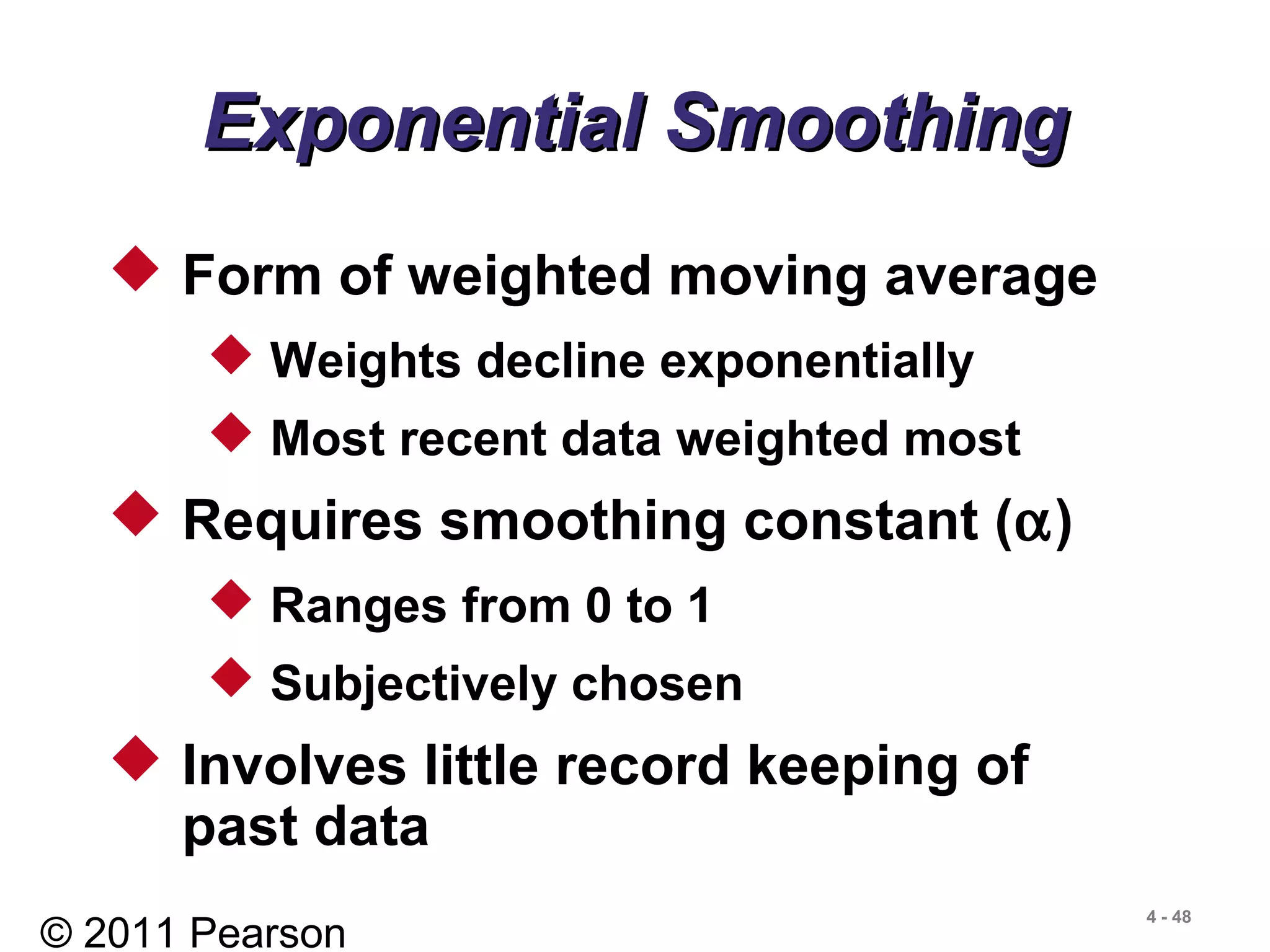
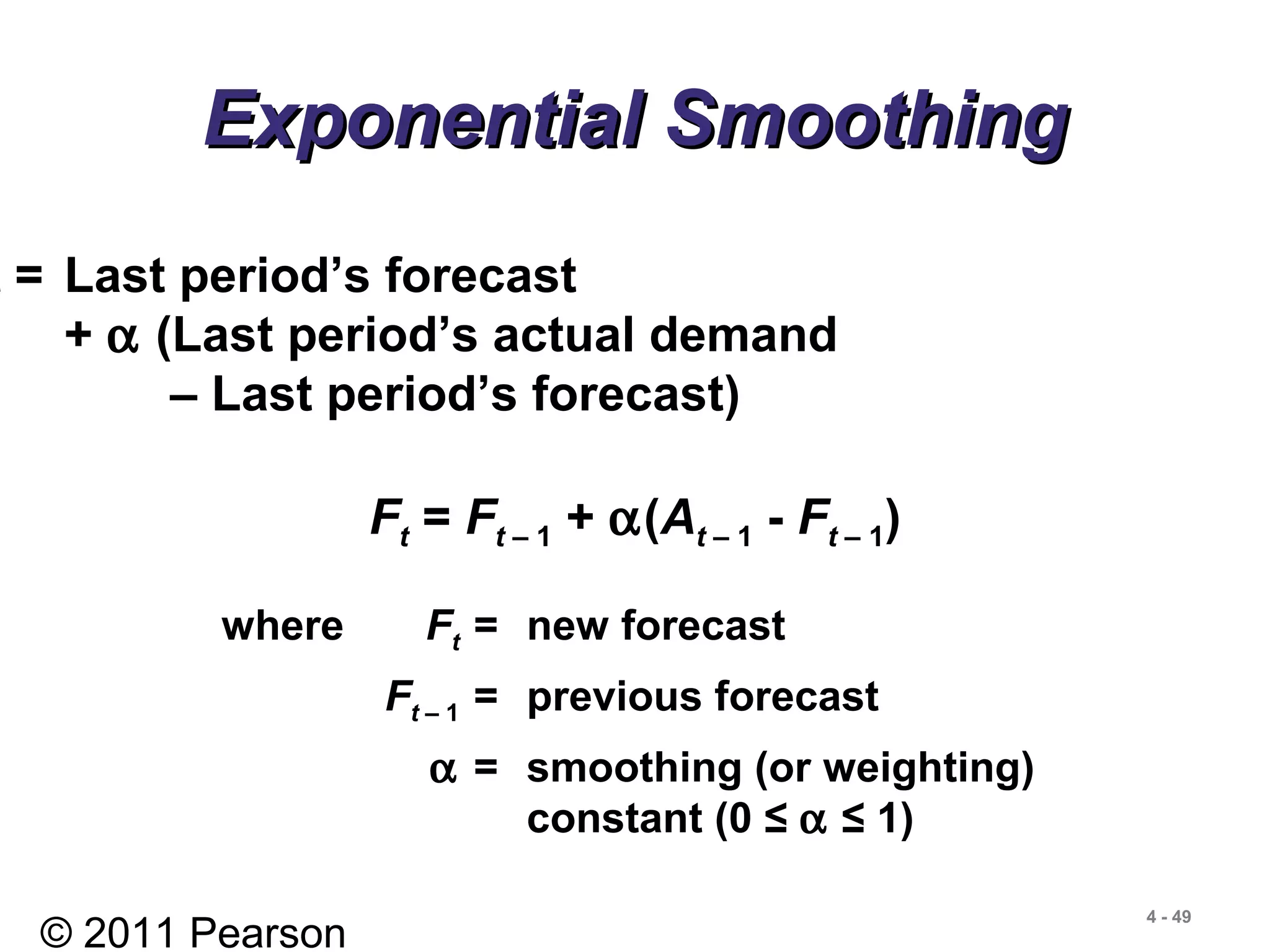
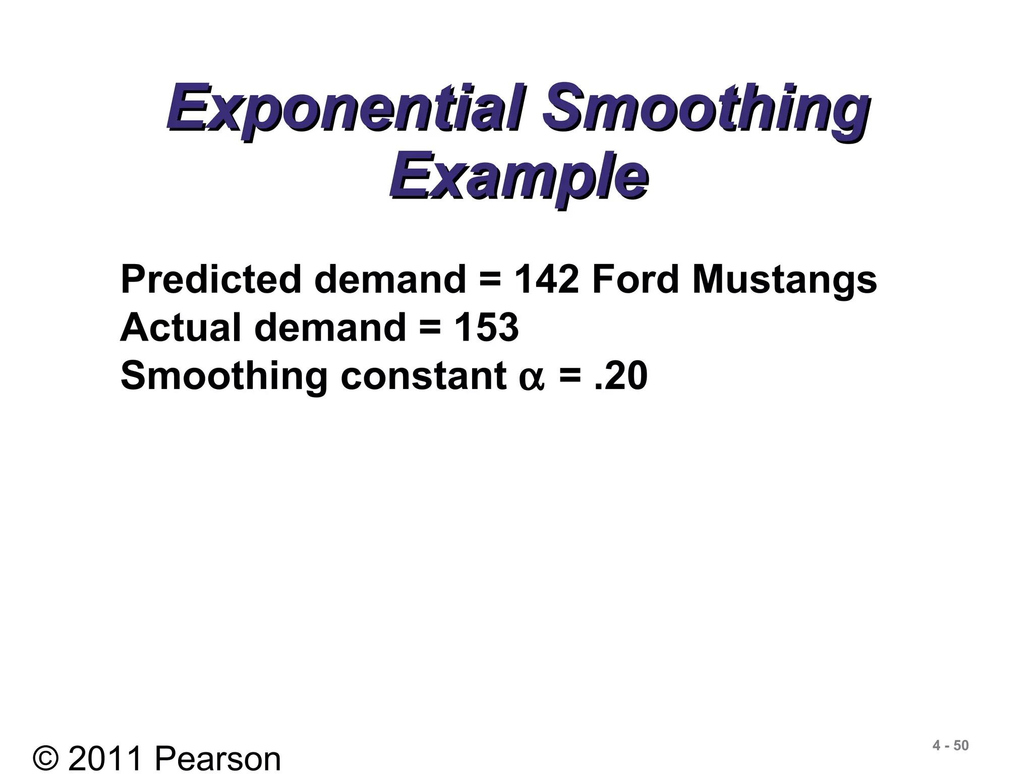
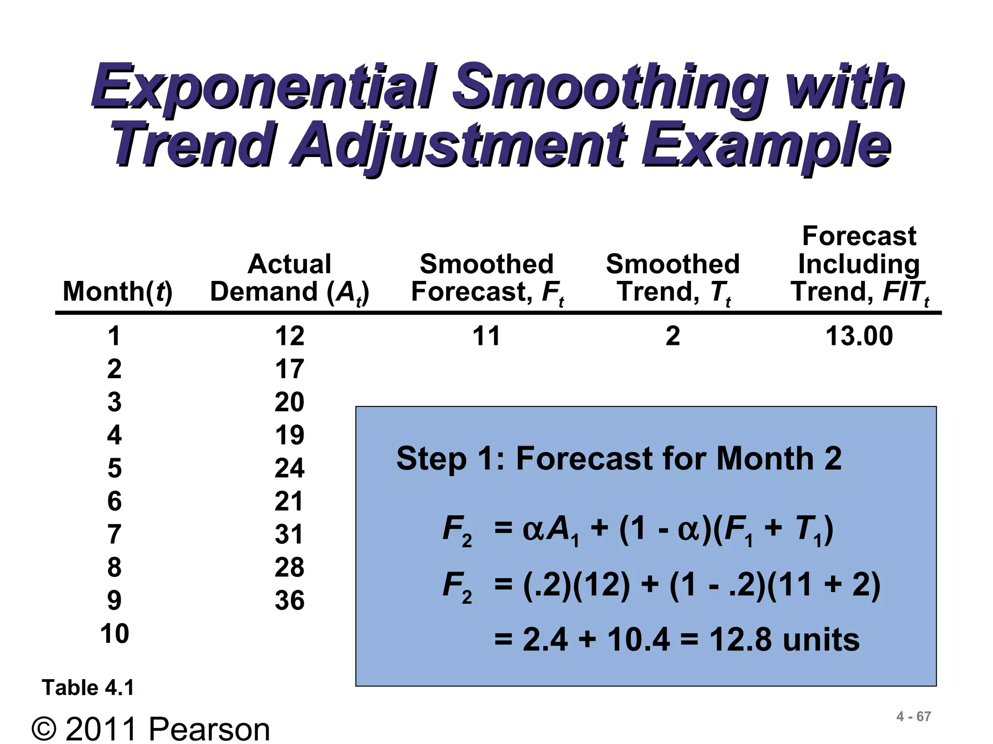
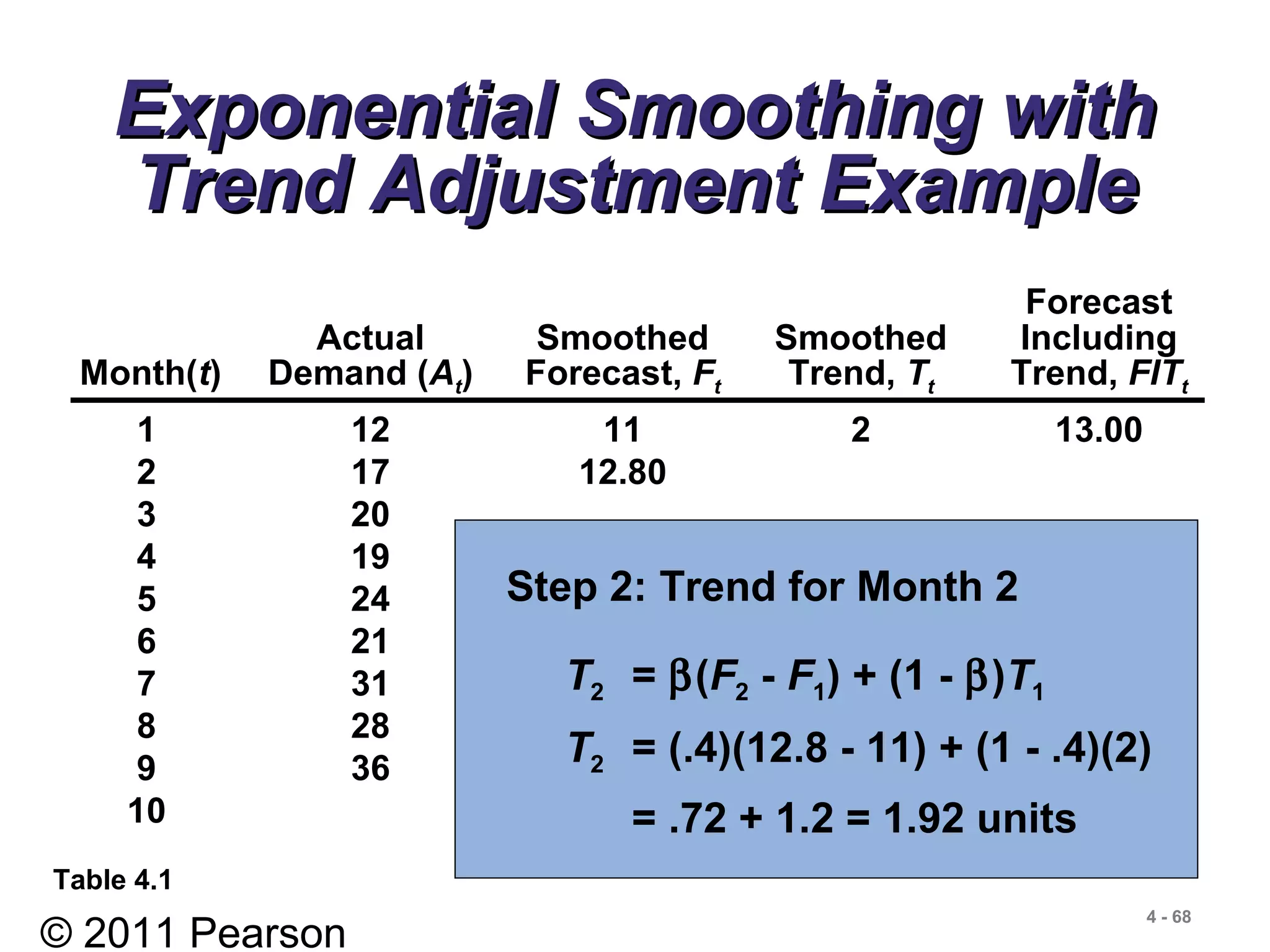
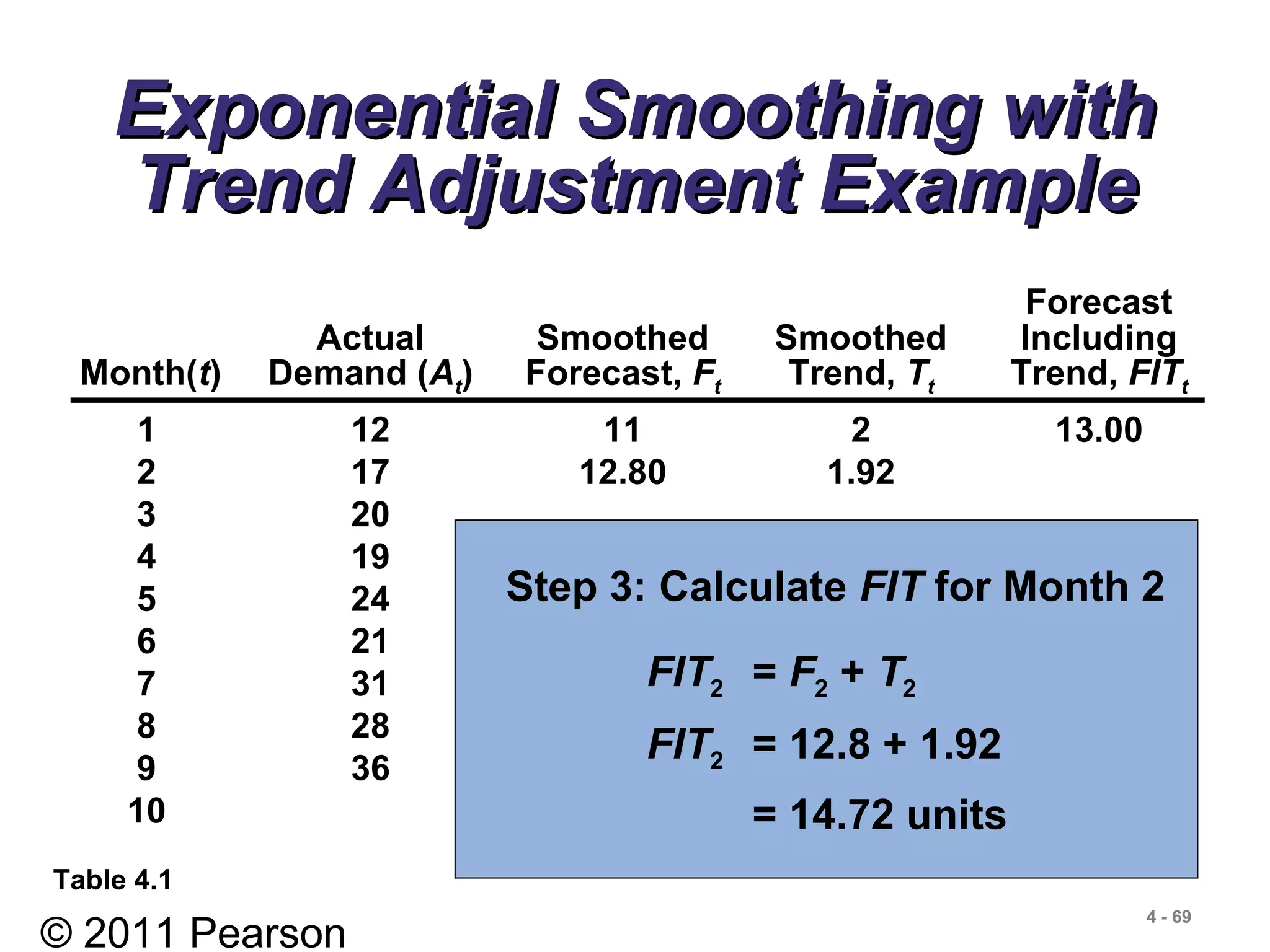
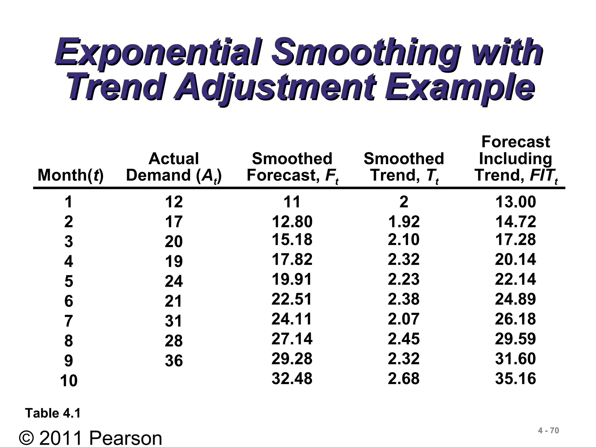
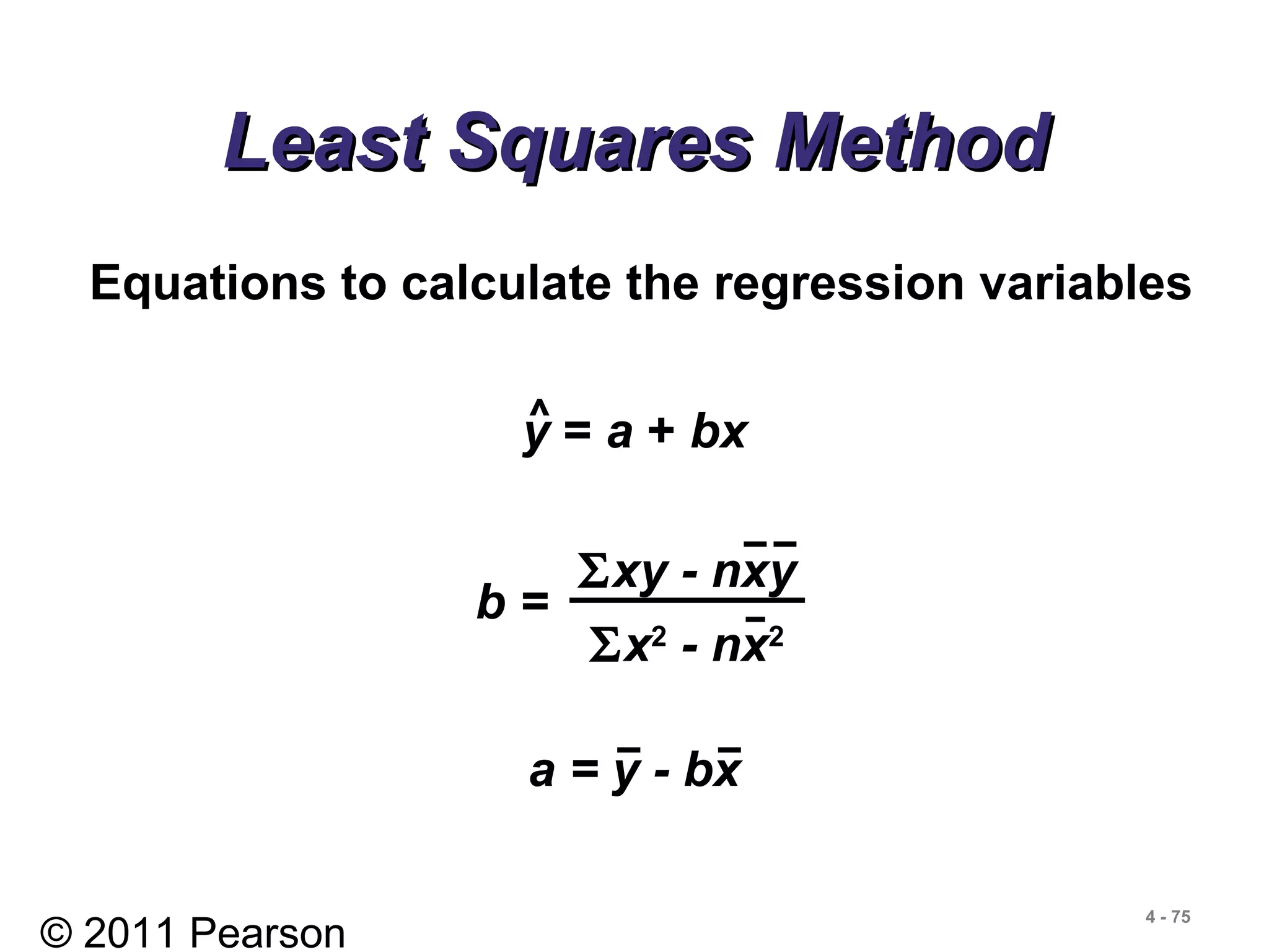
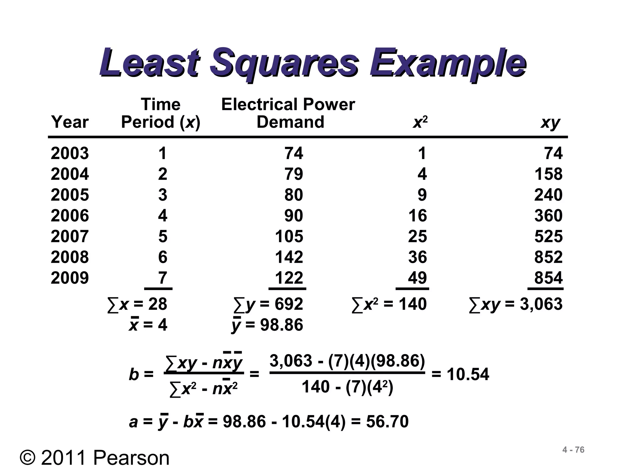
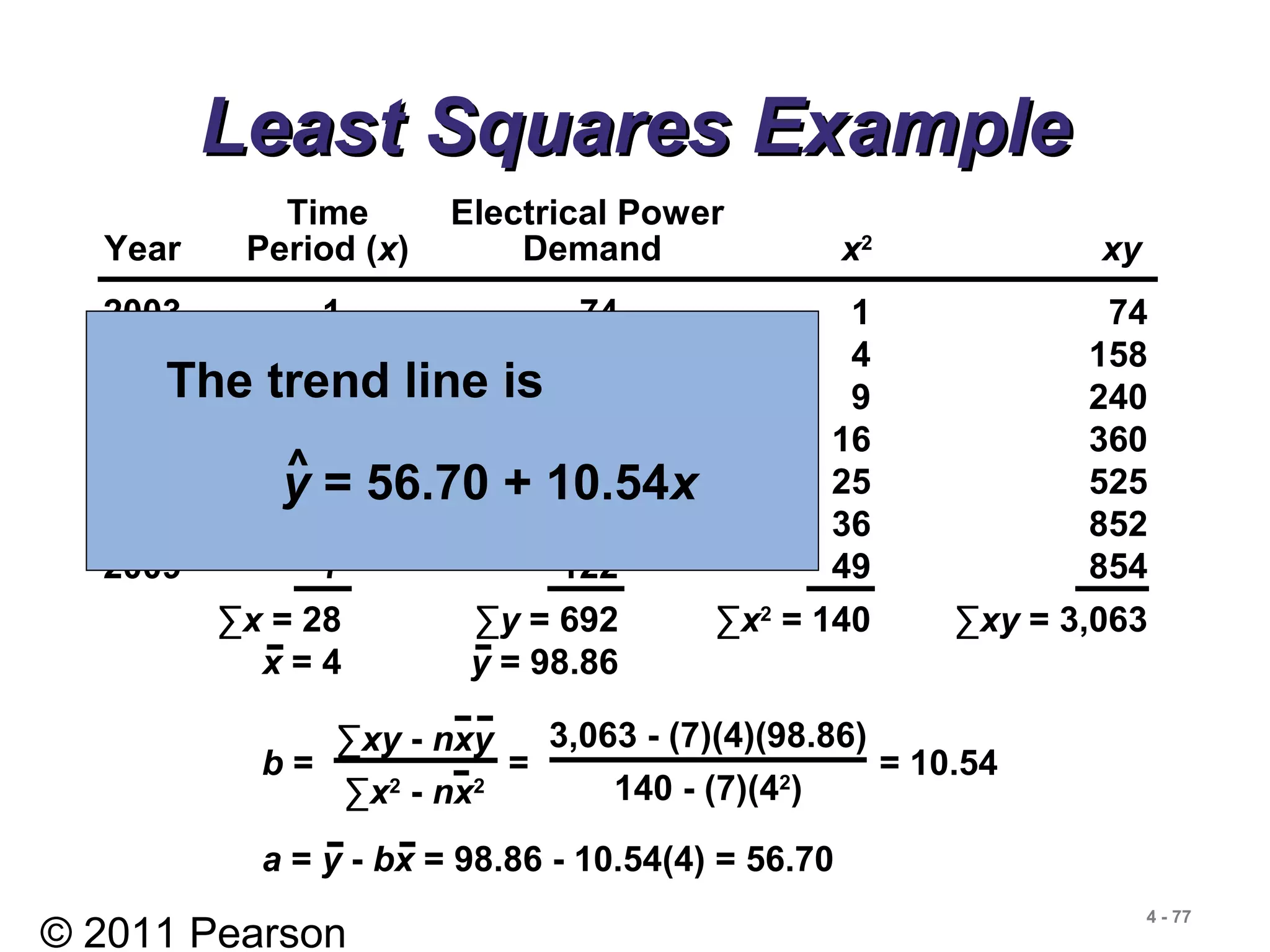
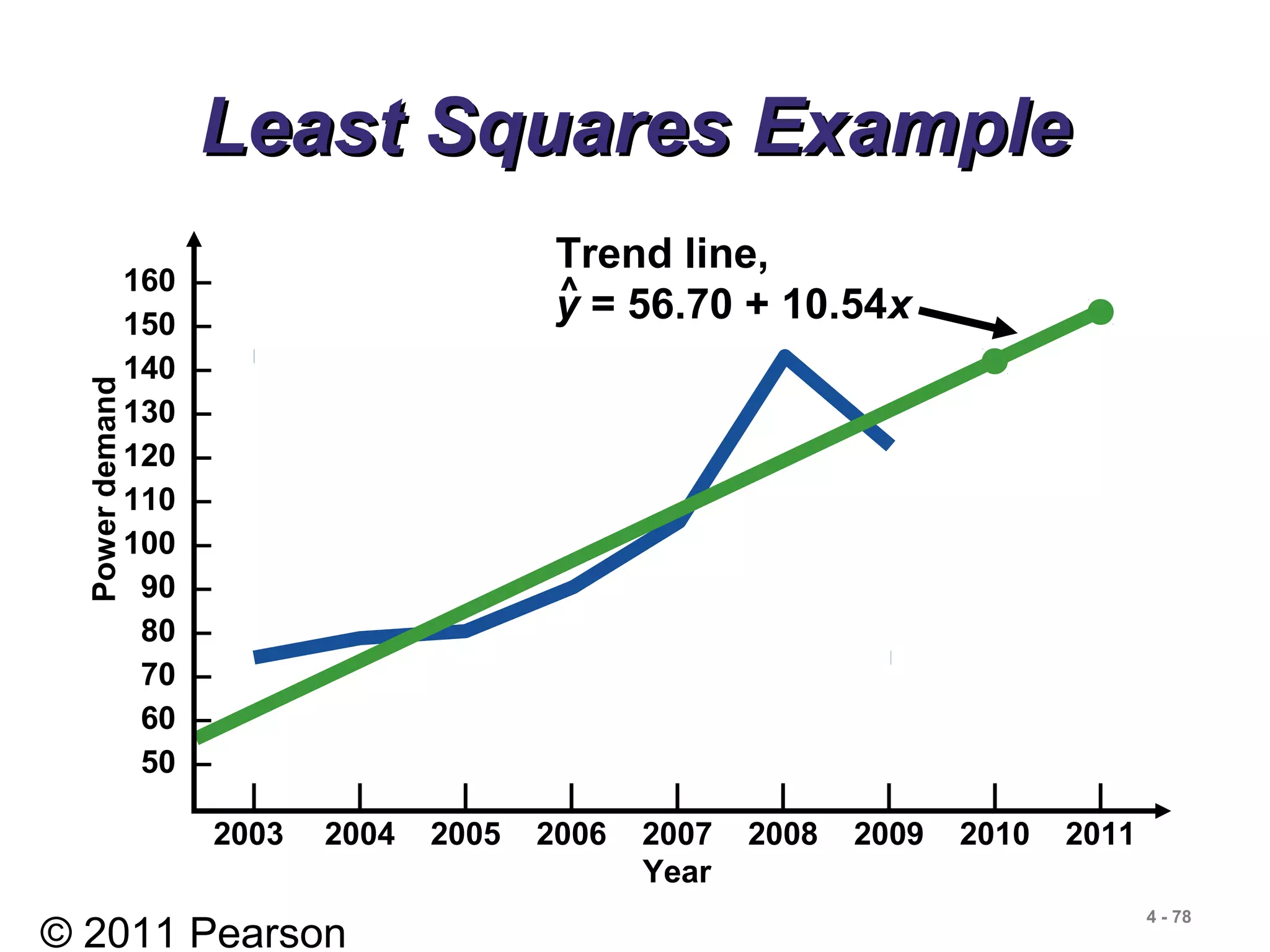
- Qualitative and quantitative forecasting methods such as jury of executive opinion, Delphi method, moving averages, and exponential smoothing.
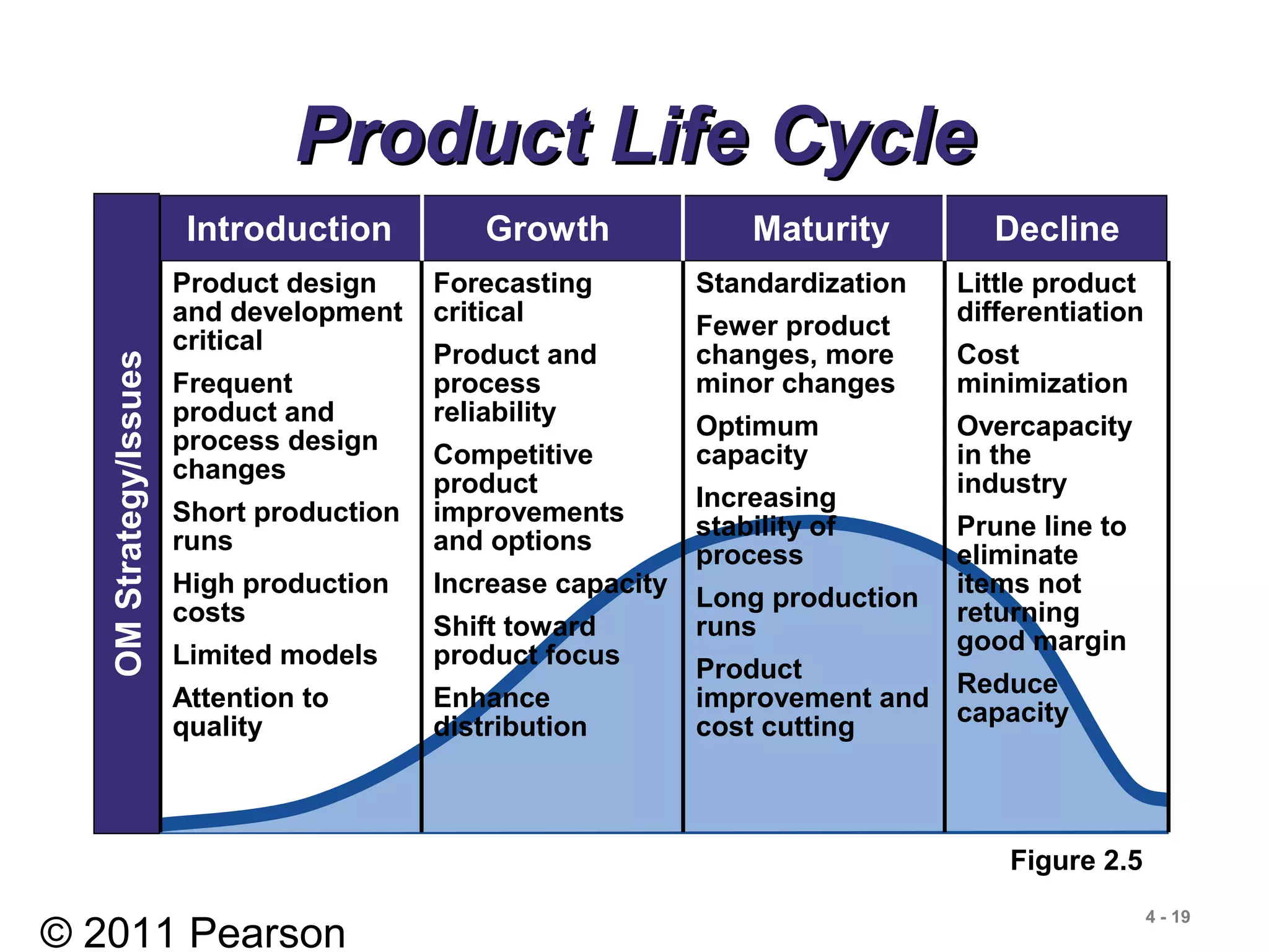
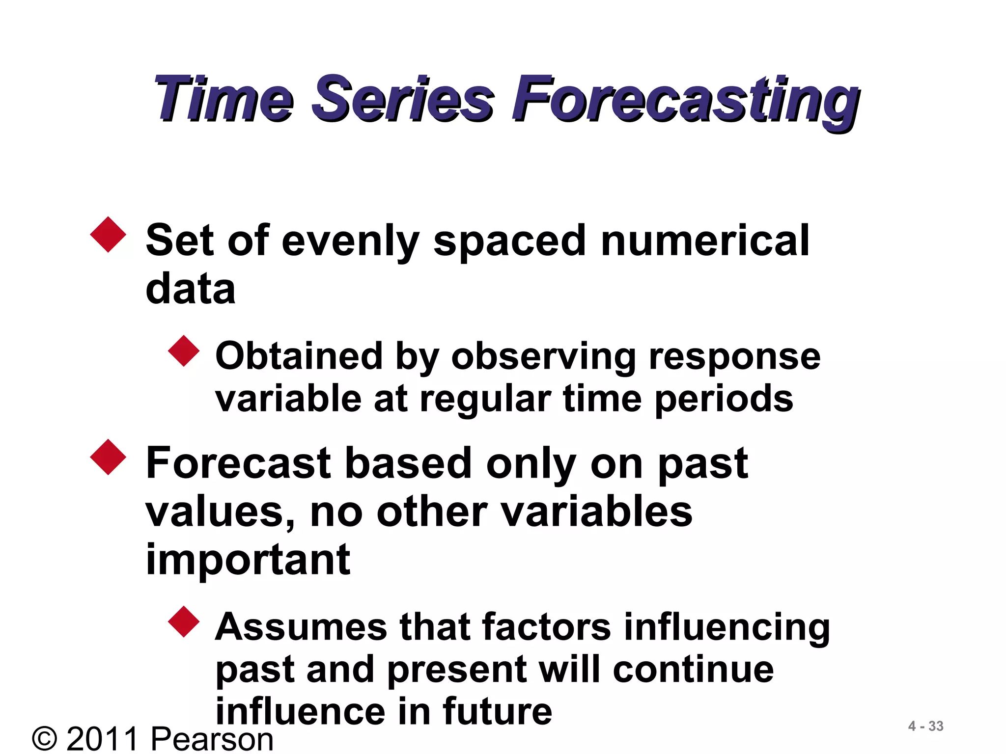
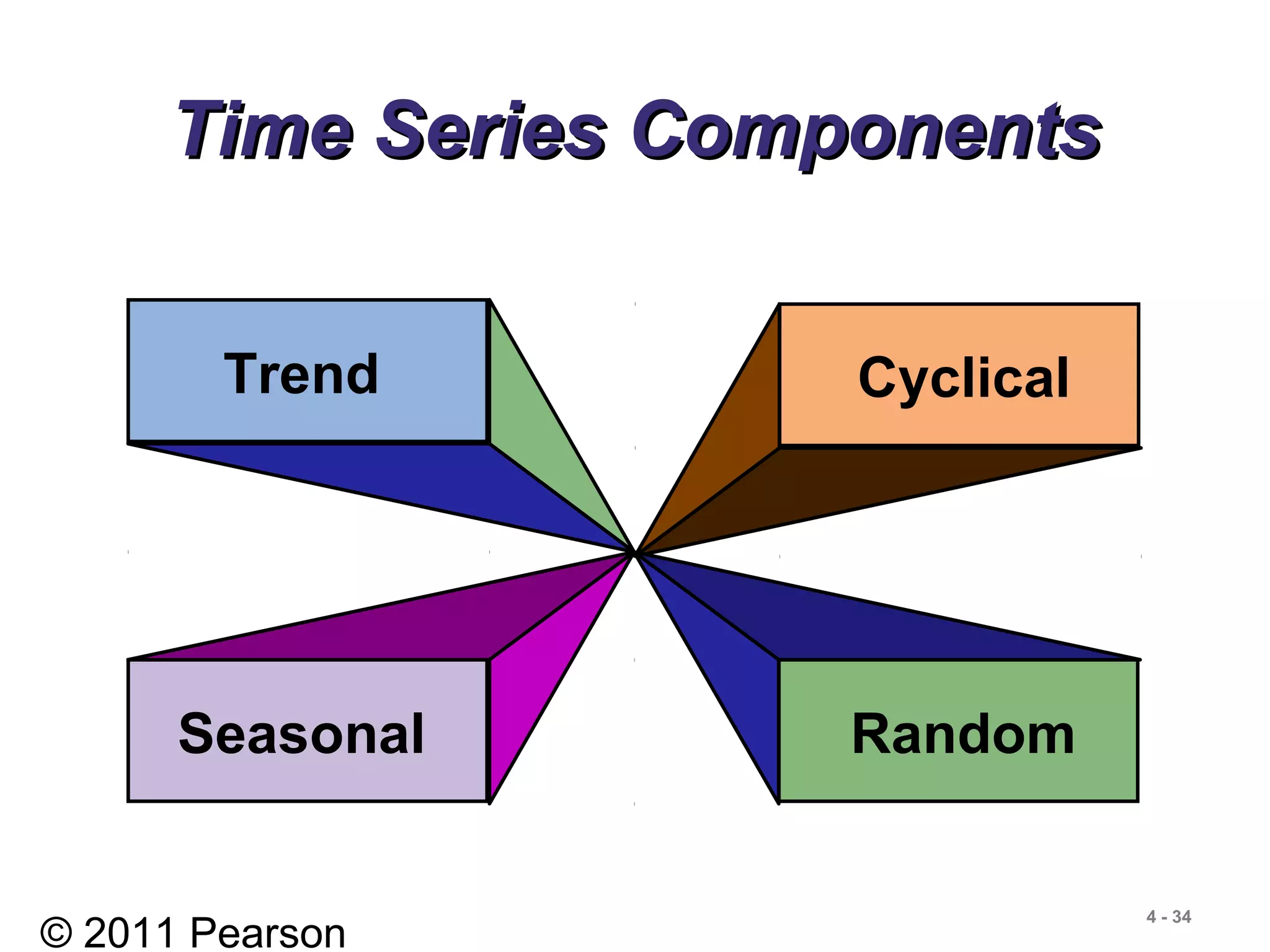
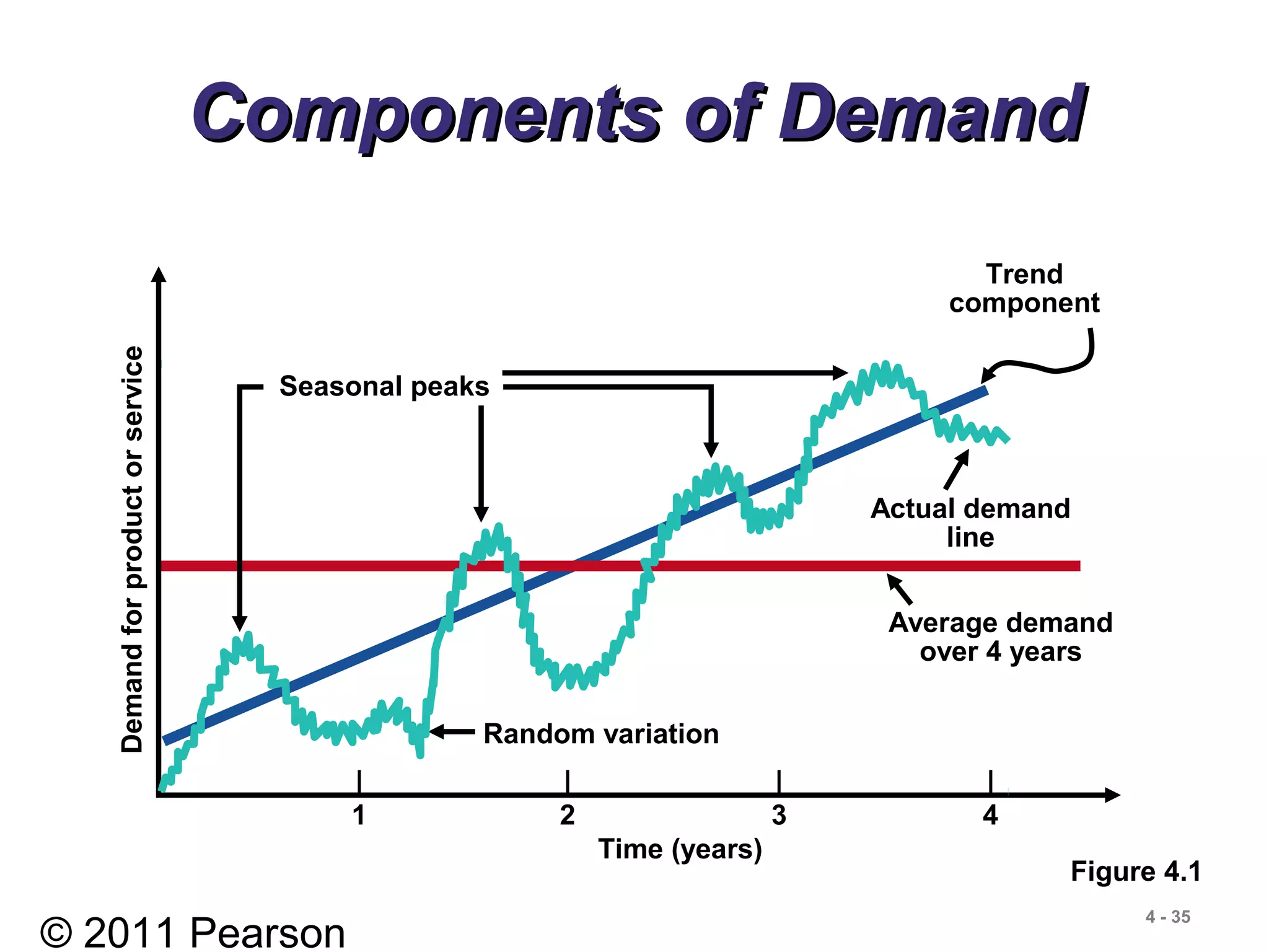
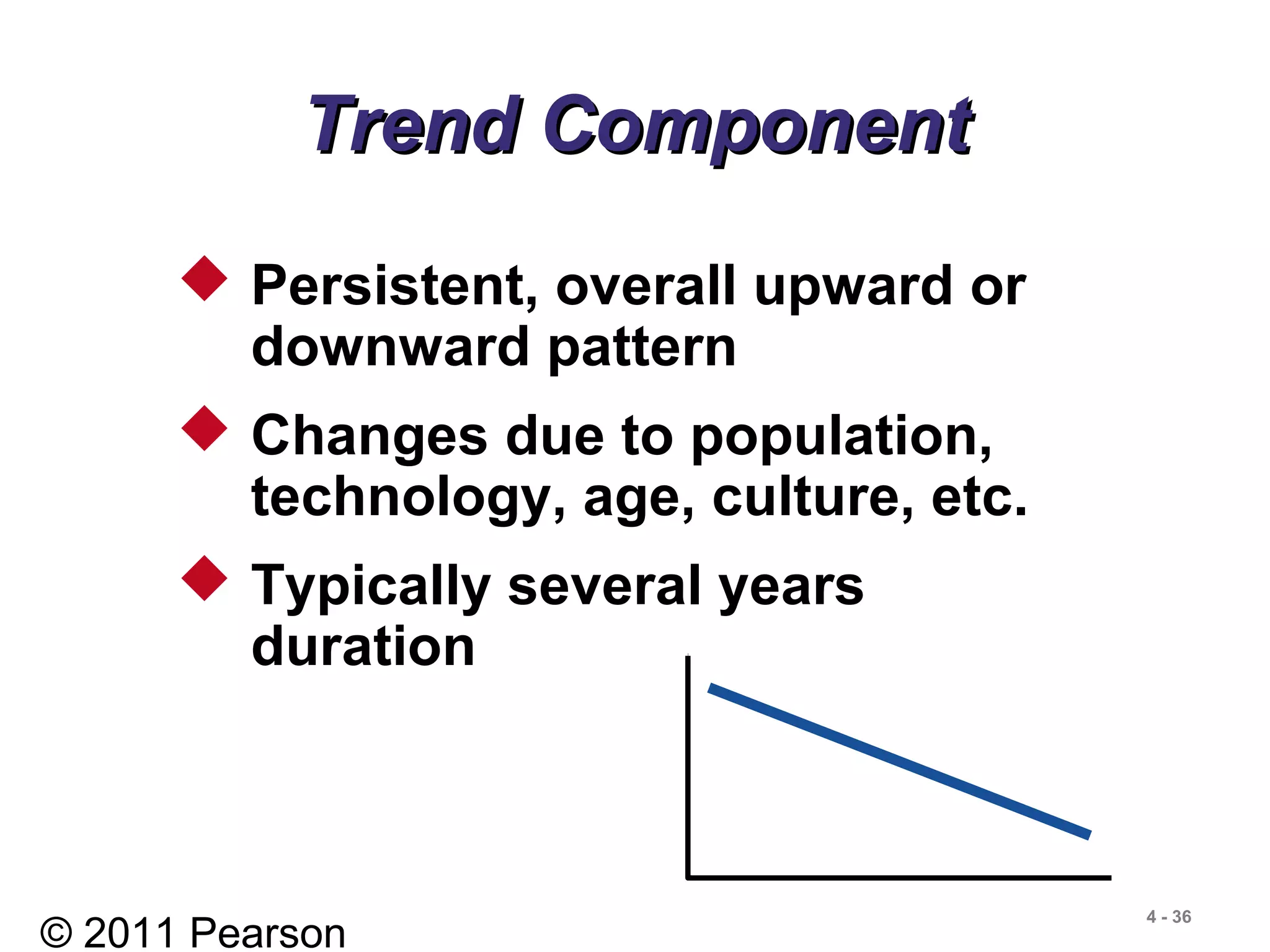
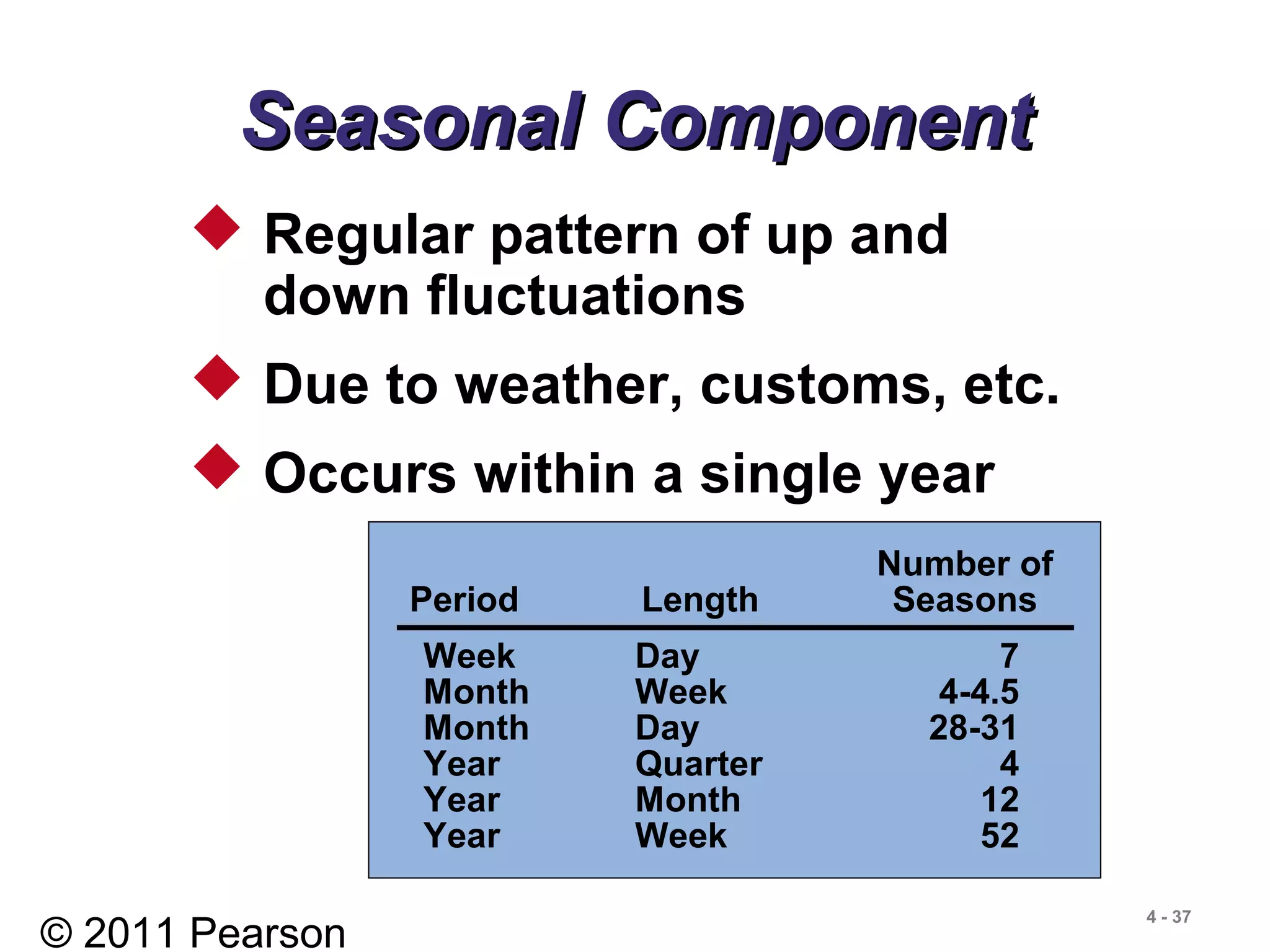
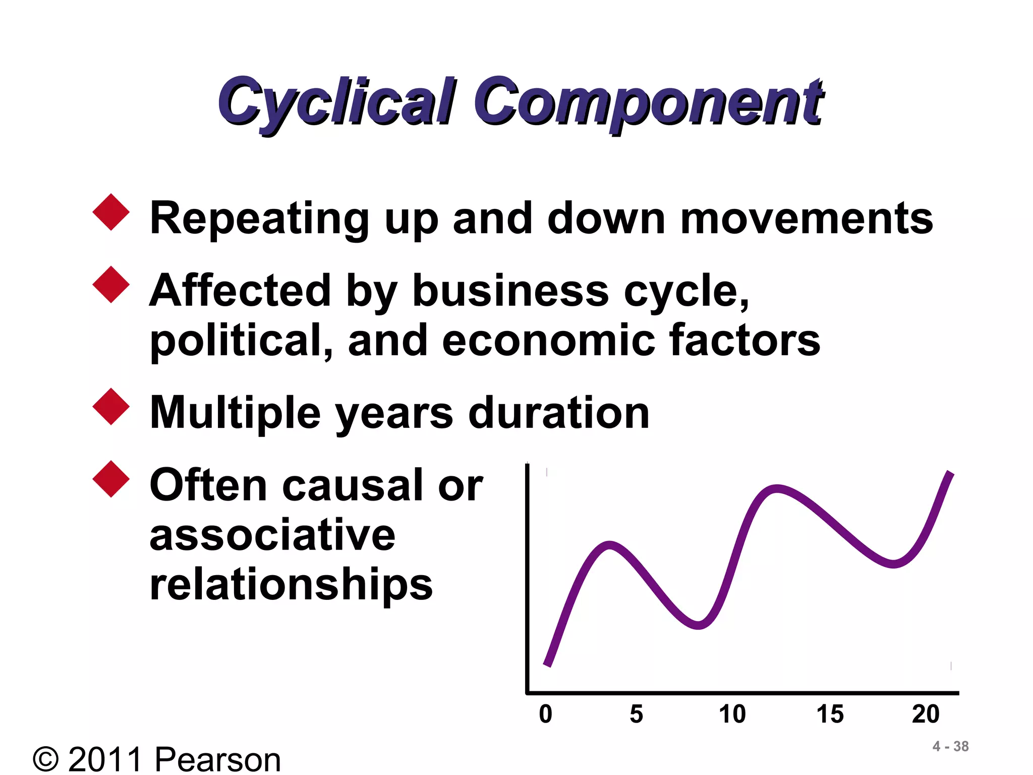
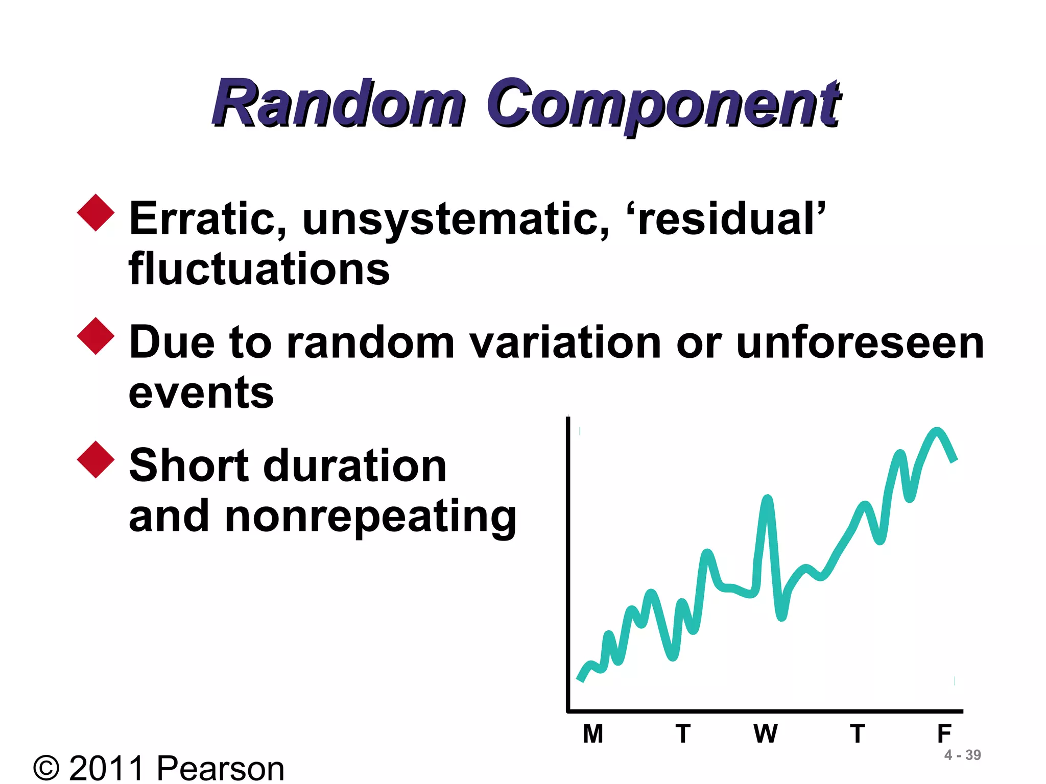
- Components of time series data including trend, seasonality, cyclicality, and randomness.
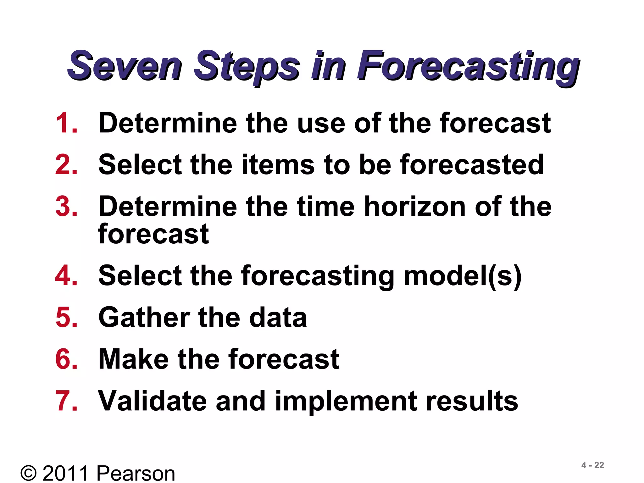
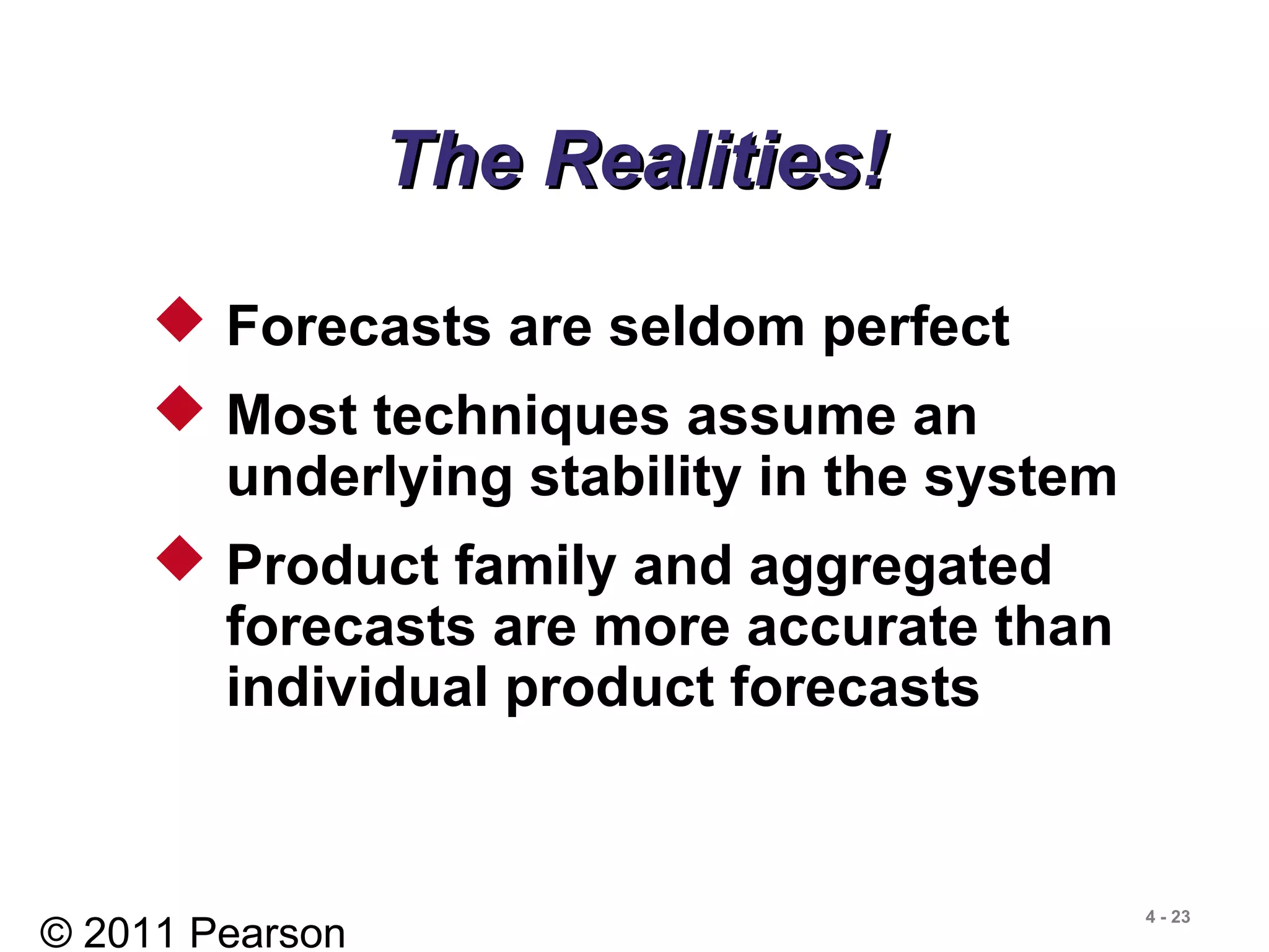
- Steps in a forecasting system and challenges with producing accurate forecasts.
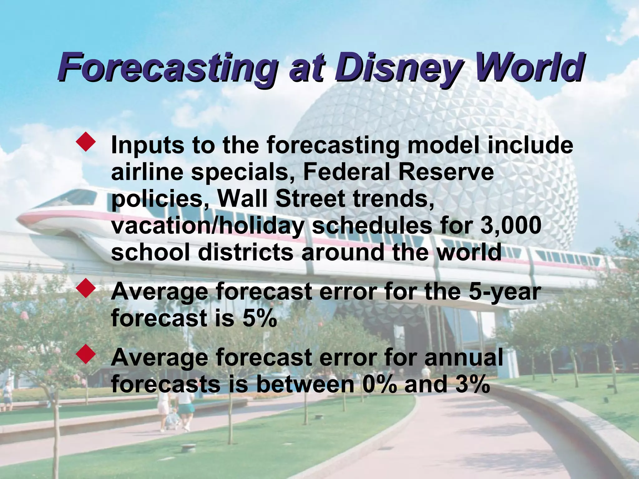
- How Disney uses forecasting across its global operations to inform decisions.


![© 2011 Pearson
4 - 45
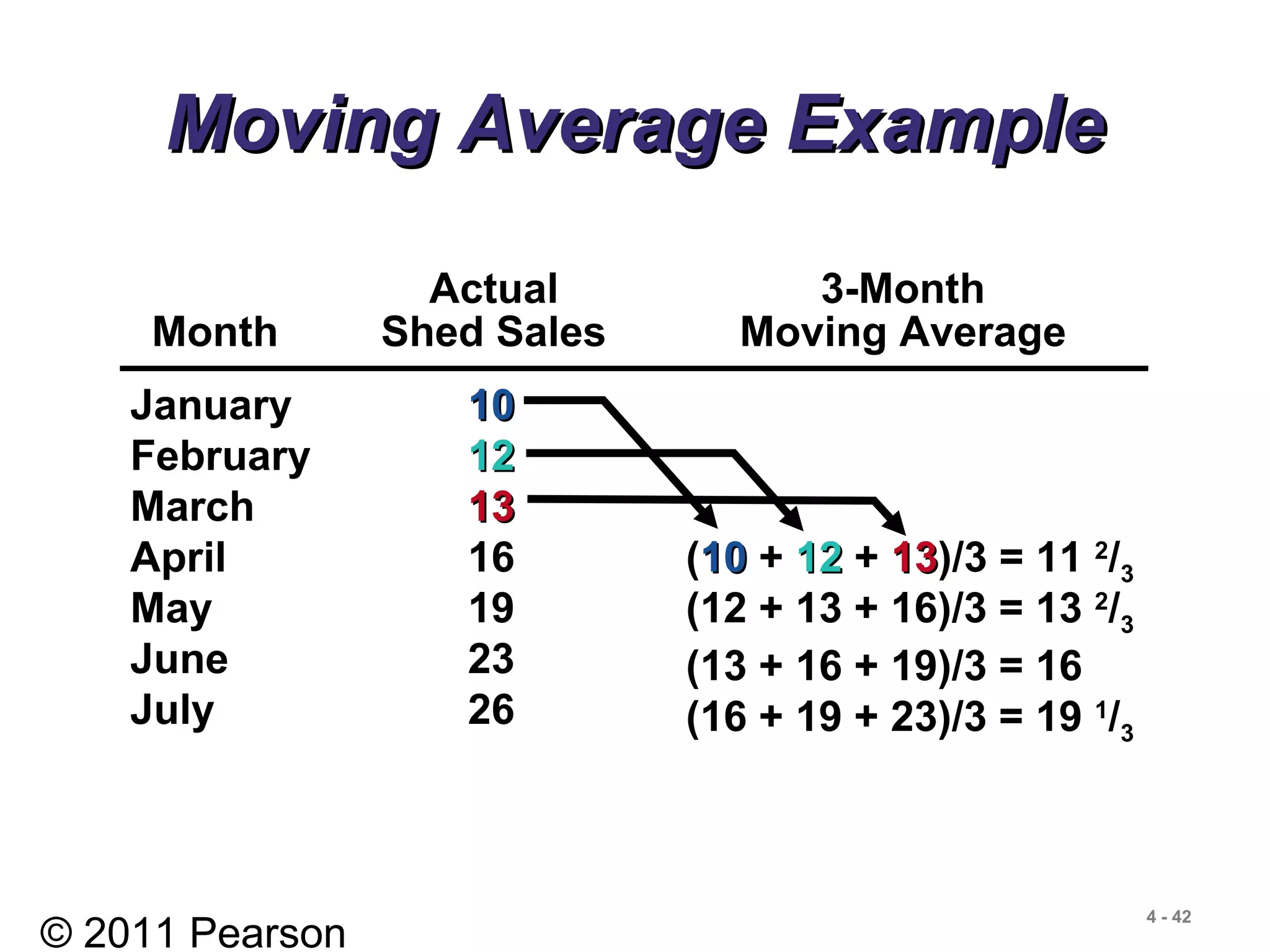
January 10
February 12
March 13
April 16
May 19
June 23
July 26
Actual 3-Month Weighted
Month Shed Sales Moving Average
[(3 x 16) + (2 x 13) + (12)]/6 = 141
/3
[(3 x 19) + (2 x 16) + (13)]/6 = 17
[(3 x 23) + (2 x 19) + (16)]/6 = 201
/2
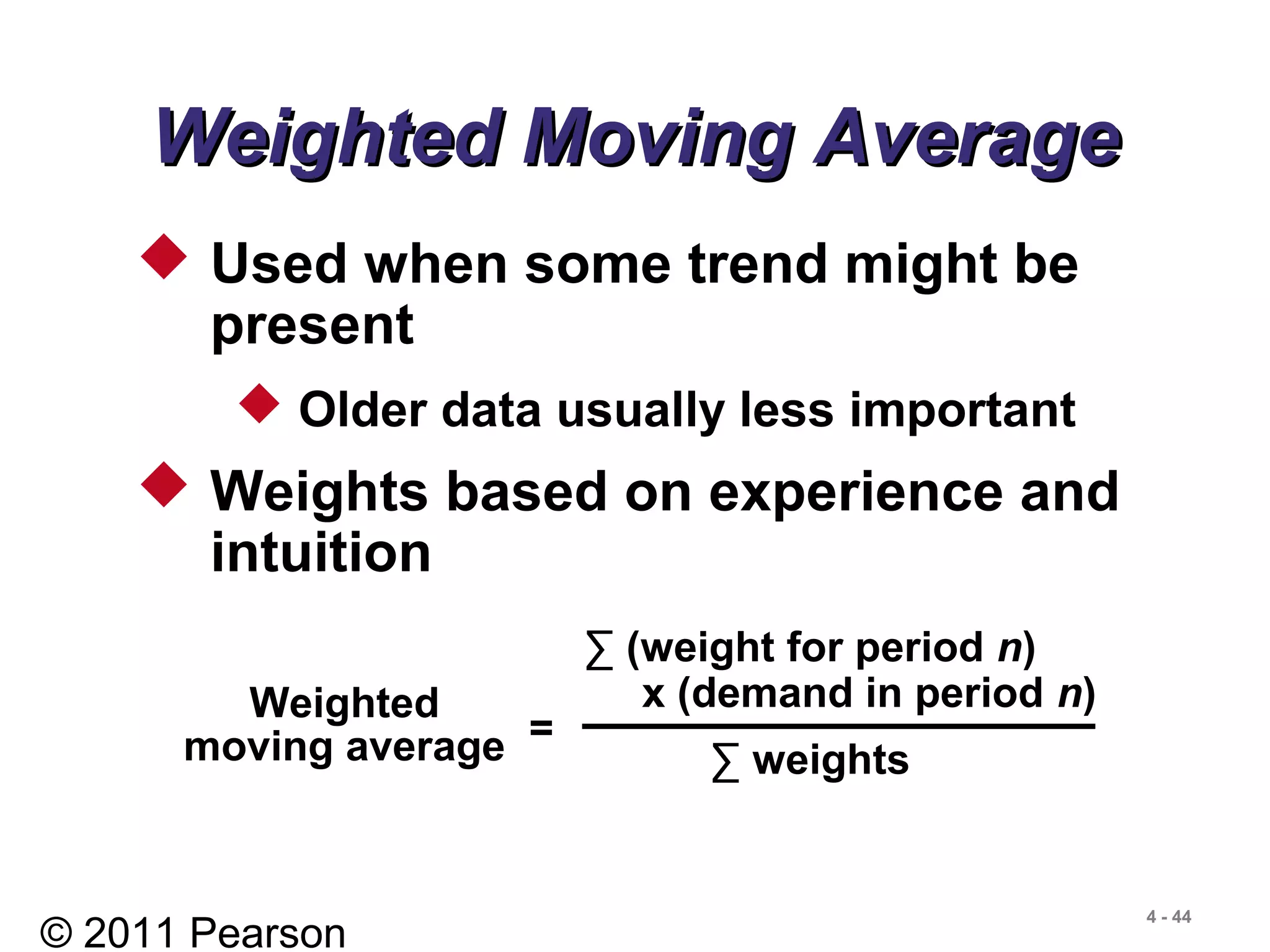
Weighted Moving AverageWeighted Moving Average
1010
1212
1313
[(3 x 1313) + (2 x 1212) + (1010)]/6 = 121
/6
Weights Applied Period
33 Last month
22 Two months ago
11 Three months ago
6 Sum of weights](https://image.slidesharecdn.com/heizerom10ch04-130523204113-phpapp02/75/360_ch04-45-2048.jpg)

![© 2011 Pearson
4 - 100
Correlation CoefficientCorrelation Coefficient
r =
nΣxy - ΣxΣy
[nΣx2
- (Σx)2
][nΣy2
- (Σy)2
]](https://image.slidesharecdn.com/heizerom10ch04-130523204113-phpapp02/75/360_ch04-99-2048.jpg)
![© 2011 Pearson
4 - 101
Correlation CoefficientCorrelation Coefficient
r =
nΣxy - ΣxΣy
[nΣx2
- (Σx)2
][nΣy2
- (Σy)2
]
y
x(a) Perfect positive
correlation:
r = +1
y
x(b) Positive
correlation:
0 < r < 1
y
x(c) No correlation:
r = 0
y
x(d) Perfect negative
correlation:
r = -1](https://image.slidesharecdn.com/heizerom10ch04-130523204113-phpapp02/75/360_ch04-100-2048.jpg)