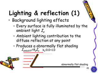
Downloaded 179 times

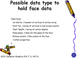
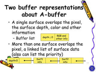
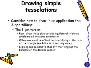
![OpenGL and Concave
Polygons
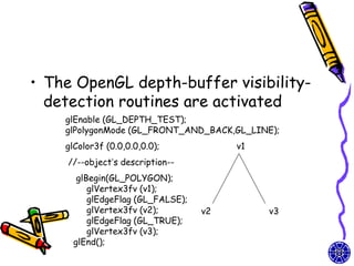
• A tessellator object in the GLU
library can tessellate a given polygon
into flat convex polygons
– Draw a simple polygon without holes
• basic idea is to describe a contour
mytess = gluNewTess(); //include
gluTessProperty()
gluTessBeginPolygon(mytess, NULL); //send them off to be rendered
gluTessBeginContour(mytess);// draw contour (outside)
for(i=0; i < n_vertices; i++)
glTessVertex(mytess,vertex[i],vertex[i]);
gluTessEndContour();
gluTessEndPolygon(mytess);](https://image.slidesharecdn.com/cg-surfacedetectionilluminationmodelssurface-renderingmodels-course9-111015013406-phpapp01/85/CG-OpenGL-surface-detection-illumination-rendering-models-course-9-8-320.jpg)
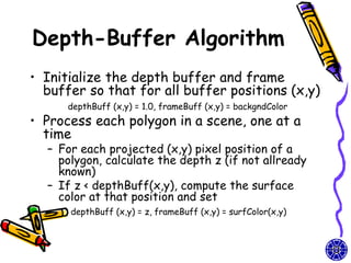
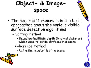
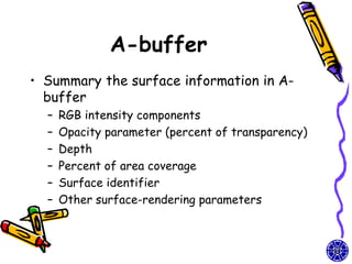
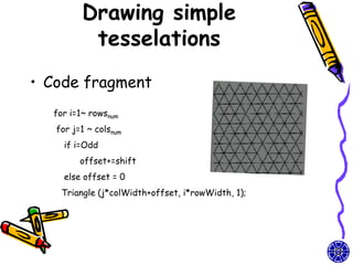
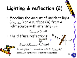
![Basic flow of depth-
buffer algorithm
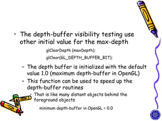
• pseudocode
for (each face F)
for (each pixel (x,y) covering the face){
depth = depth of F at (x,y);
if (depth < d[x][y]) { //F is closest so far
c = color of F at (x,y) //set the pixel color at (x,y) to c
d[x][y] = depth; //updata the depth buffer
}
}](https://image.slidesharecdn.com/cg-surfacedetectionilluminationmodelssurface-renderingmodels-course9-111015013406-phpapp01/85/CG-OpenGL-surface-detection-illumination-rendering-models-course-9-14-320.jpg)
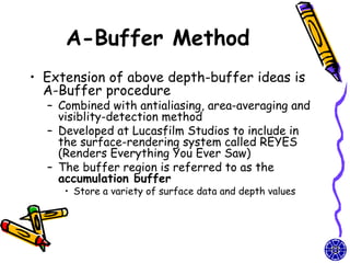
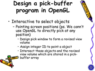
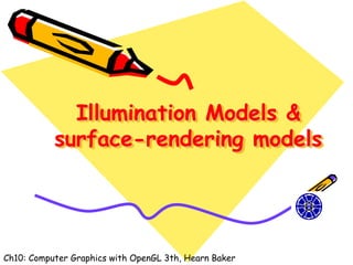
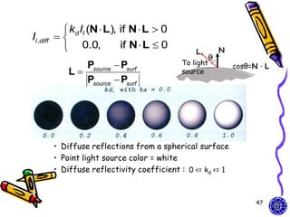
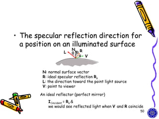
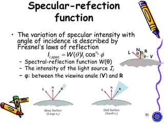
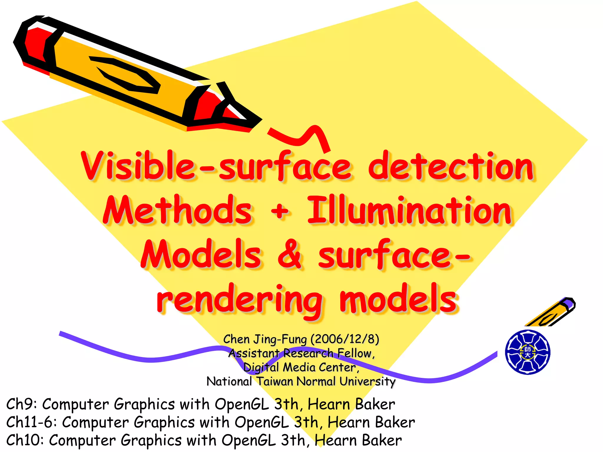
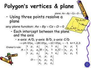
![Combined diffuse and
specular reflection
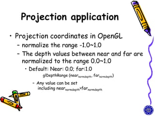
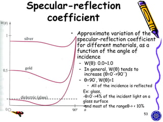
• A single point light source
I Idiff Ispec
kaIa kd Il (N L) ksIl (N H)ns
• Multiple light sources
n
I Iambdiff [Il ,diff Il ,spec ]
l 1
n
kaIa Il [kd (N Ll ) ks (N Hl )ns ]
l 1
57](https://image.slidesharecdn.com/cg-surfacedetectionilluminationmodelssurface-renderingmodels-course9-111015013406-phpapp01/85/CG-OpenGL-surface-detection-illumination-rendering-models-course-9-57-320.jpg)
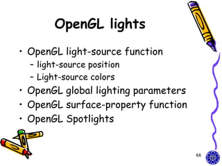
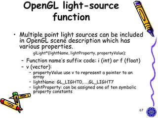
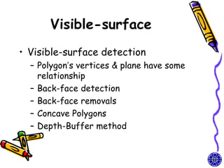
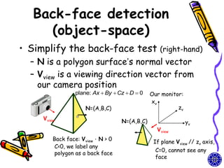
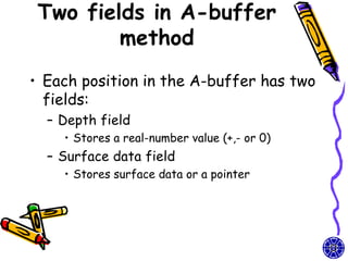
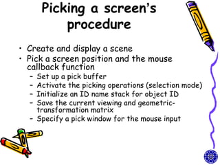
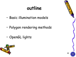
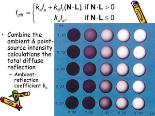
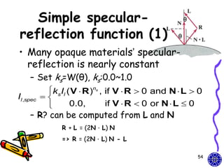
![OpenGL light-source
position
// light1 is designated as a local source at (2.0,0.0,3.0)
GLfloat light1PosType [ ] = {2.0, 0.0, 3.0, 1.0}
//light2 is a distant source with light emission in –y axis
GLfloat light2PosType [ ] = {0.0, 1.0, 0.0, 0.0}
glLightfv(GL_LIGHT1, GL_POSITION, light1PosType);
glEnable(GL_LIGHT1); // turn on light1
….
68](https://image.slidesharecdn.com/cg-surfacedetectionilluminationmodelssurface-renderingmodels-course9-111015013406-phpapp01/85/CG-OpenGL-surface-detection-illumination-rendering-models-course-9-68-320.jpg)
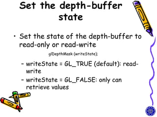
![OpenGL Light-source
colors
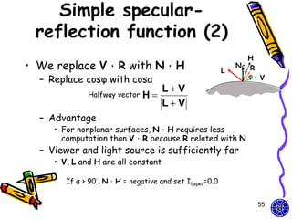
• Light-source colors (R,G,B,A)
– The symbolic color-property
• GL_AMBIENT, GL_DIFFUSE and
GL_SPECULAR
GLfloat color1 [ ] = {0.0, 0.0, 0.0, 1.0}//black
GLfloat color2 [ ] = {1.0, 1.0, 1.0, 1.0}//white
glLightfv (GL_LIGHT3, GL_AMBIENT, color1);
…
69](https://image.slidesharecdn.com/cg-surfacedetectionilluminationmodelssurface-renderingmodels-course9-111015013406-phpapp01/85/CG-OpenGL-surface-detection-illumination-rendering-models-course-9-69-320.jpg)
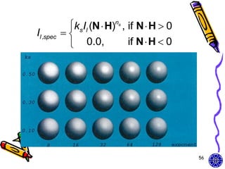
![OpenGL global lighting
parameters
• OpenGL lighting parameters can be
specified at the global level
glLightModel* (paramName, ParamValue);
– Besides the ambient color for individual light
sources, we can also set it to be background
lighting as a global value
• Ex: set background lighting to a low-intensity dark-
blue color and an alpha value = 1.0
globalAmbient [ ] = {0.0, 0.0, 0.3, 1.0}
glLightModelfv(GL_LIGHT_MODEL_AMBIENT, globalAmbient);
Default global Ambient color = (0.2,0.2,0.2,1.0)
//dark gray
71](https://image.slidesharecdn.com/cg-surfacedetectionilluminationmodelssurface-renderingmodels-course9-111015013406-phpapp01/85/CG-OpenGL-surface-detection-illumination-rendering-models-course-9-71-320.jpg)
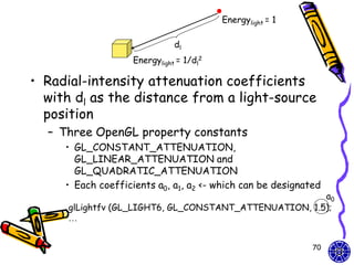
![Ambient & diffuse realization
• The ambient and diffuse coefficients
should be assigned the same vector values
– GL_AMBIENT_AND_DIFFUSE
• To set the specular-reflection exponent
– GL_SHININESS
• The range of the value : 0 ~ 128
diffuseCoeff [ ] = {0.2, 0.4, 0.9, 1.0};//light-blue color
specularCoeff [ ] = {1.0, 1.0, 1.0, 1.0};//white light
glMaterialfv (GL_FRONT_AND_BACK,
GL_AMBIENT_AND_DIFFUSE, diffuseCoeff);
glMaterialfv(GL_FRONT_AND_BACK, GL_SPECULAR, specularCoeff);
glMaterialfv(GL_FRONT_AND_BACK, GL_SHININESS, 25.0);
73](https://image.slidesharecdn.com/cg-surfacedetectionilluminationmodelssurface-renderingmodels-course9-111015013406-phpapp01/85/CG-OpenGL-surface-detection-illumination-rendering-models-course-9-73-320.jpg)
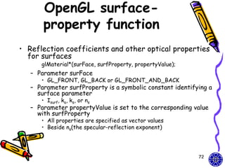
![OpenGL Spotlights
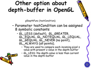
• Spotlights is directional light sources
– Three OpenGL property constants for
directional effects
• GL_SPOT_DIRECTION, GL_SPOT_CUTOFF
and GL_SPOT_EXPONENT
– Ex: θl = 30°, cone axis= x-axis and the attenuation
exponent = 2.5
GLfloat dirVector [ ] = {1.0, 0.0, 0.0}; To object Vobj
glLightfv(GL_LIGHT4, GL_SPOT_DIRECTION, dirVector); vertex
α
glLightf(GL_LIGHT4, GL_SPOT_CUTOFF, 30.0);
glLightf(GL_LIGHT4, GL_SPOT_EXPONENT, 2.5);
cone axis
Light
source θl
74
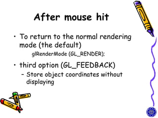
demo](https://image.slidesharecdn.com/cg-surfacedetectionilluminationmodelssurface-renderingmodels-course9-111015013406-phpapp01/85/CG-OpenGL-surface-detection-illumination-rendering-models-course-9-74-320.jpg)

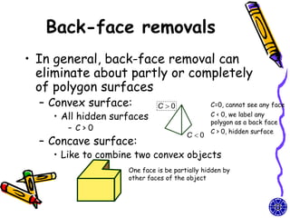
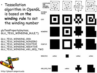
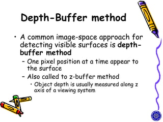
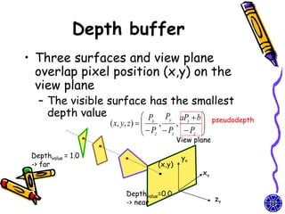
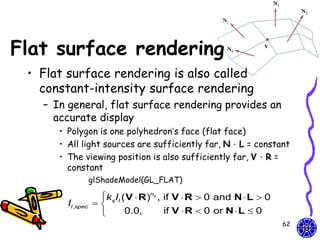
The document discusses methods for visible-surface detection in computer graphics, including back-face detection and removal, depth-buffer techniques, and image-space versus object-space approaches. It also covers illumination models, such as ambient and diffuse reflections, along with rendering methods in OpenGL for polygon rendering. Additionally, it touches on techniques like tessellation and design considerations for interactive object selection using a pick-buffer.