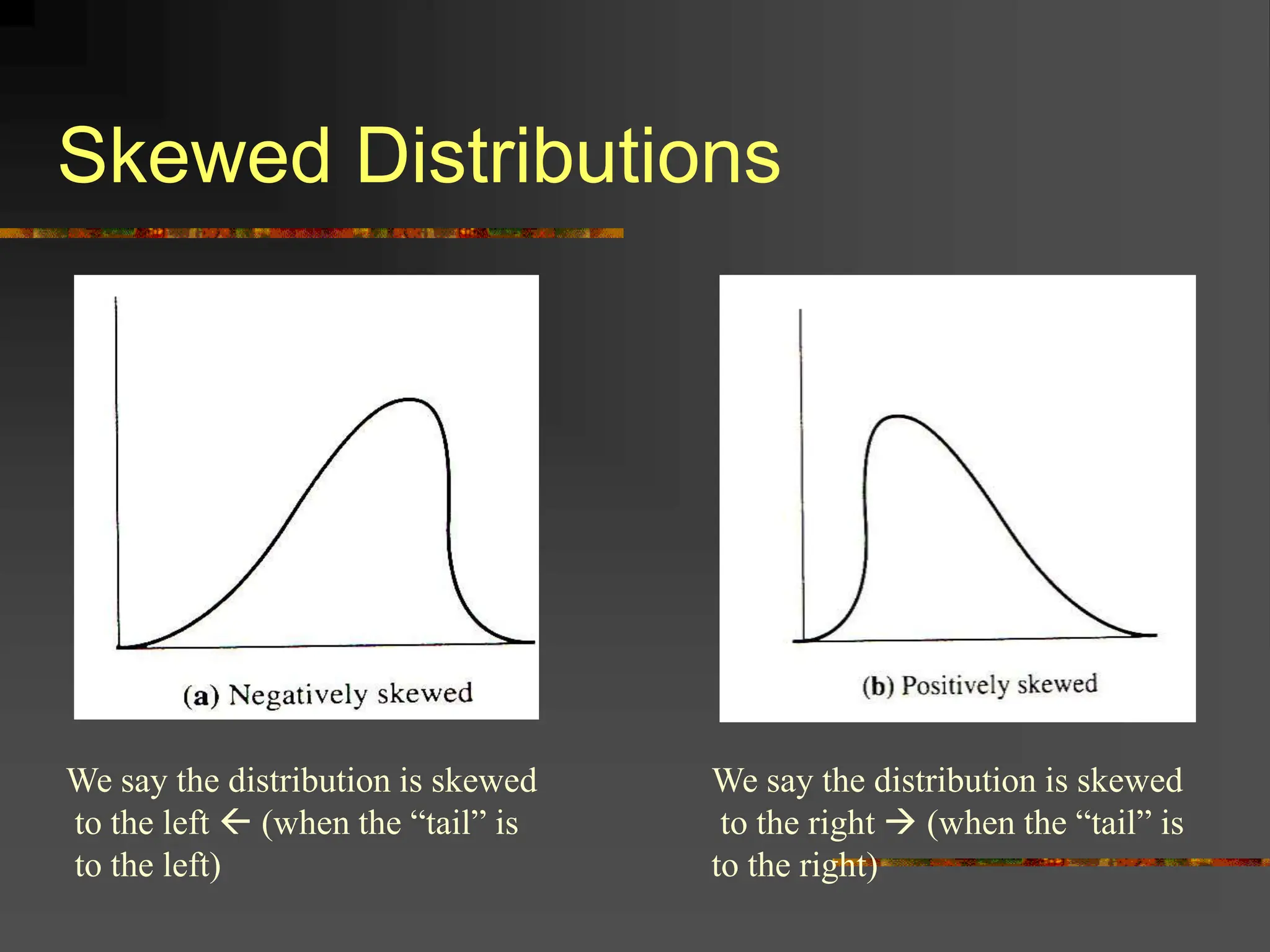
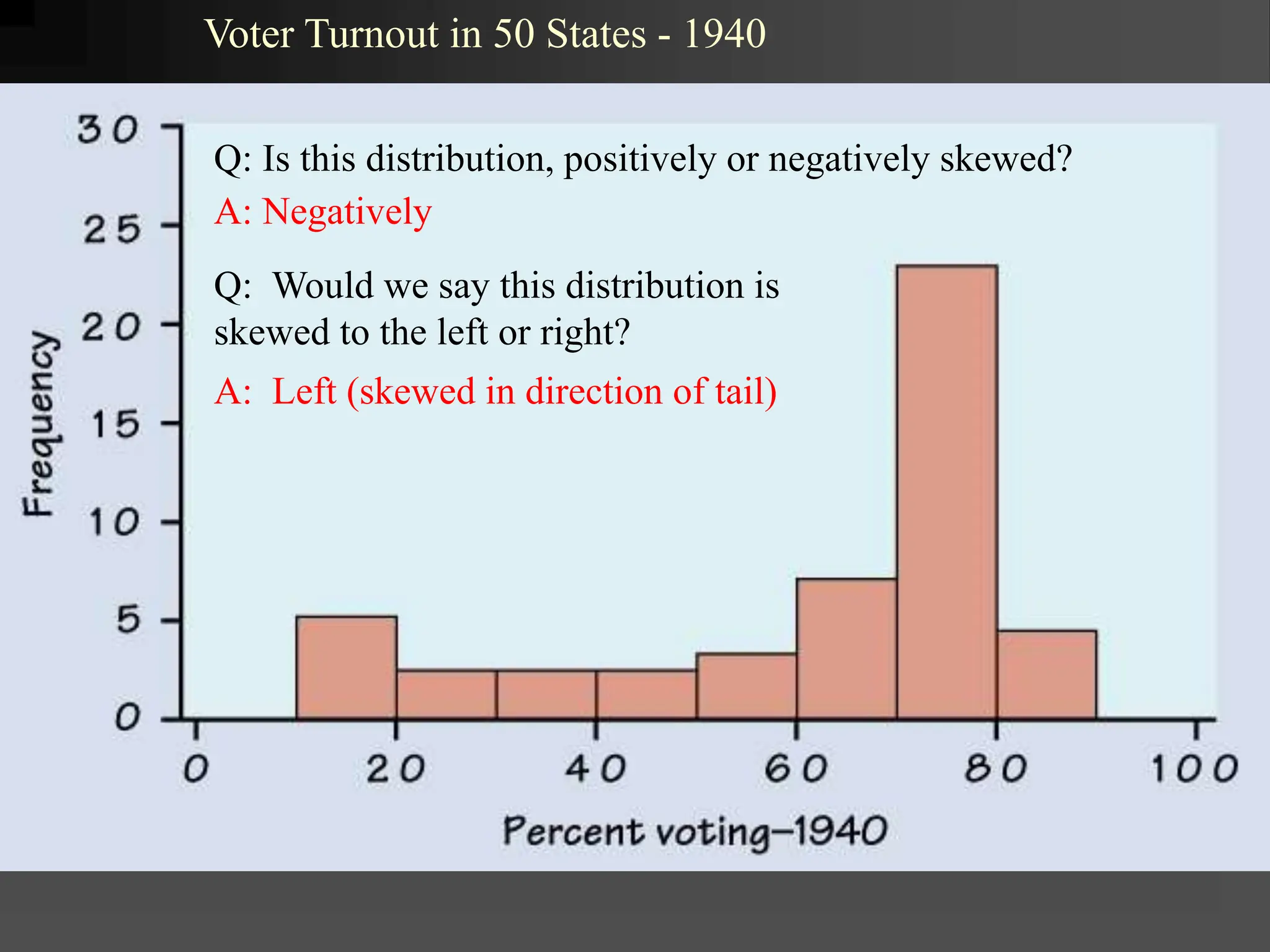
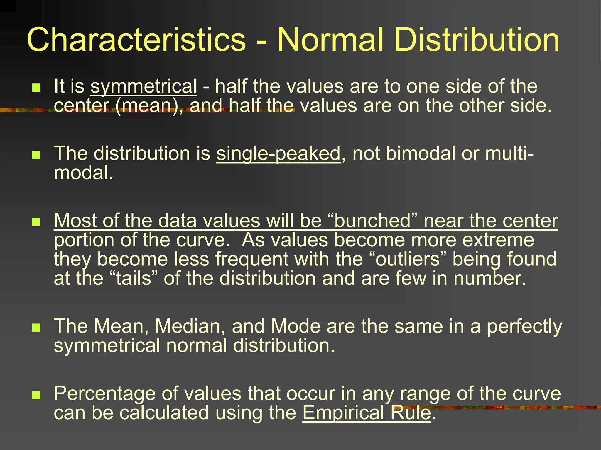
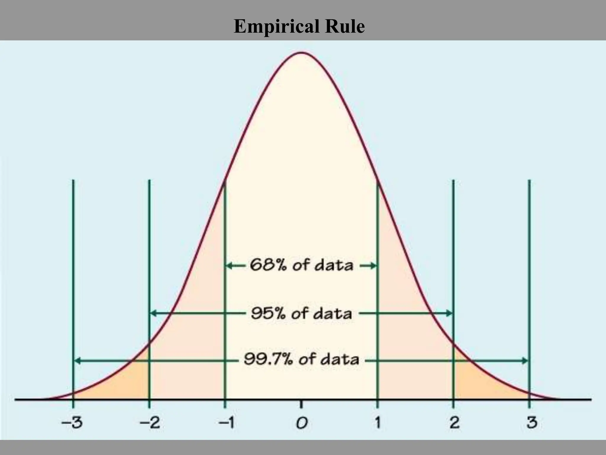
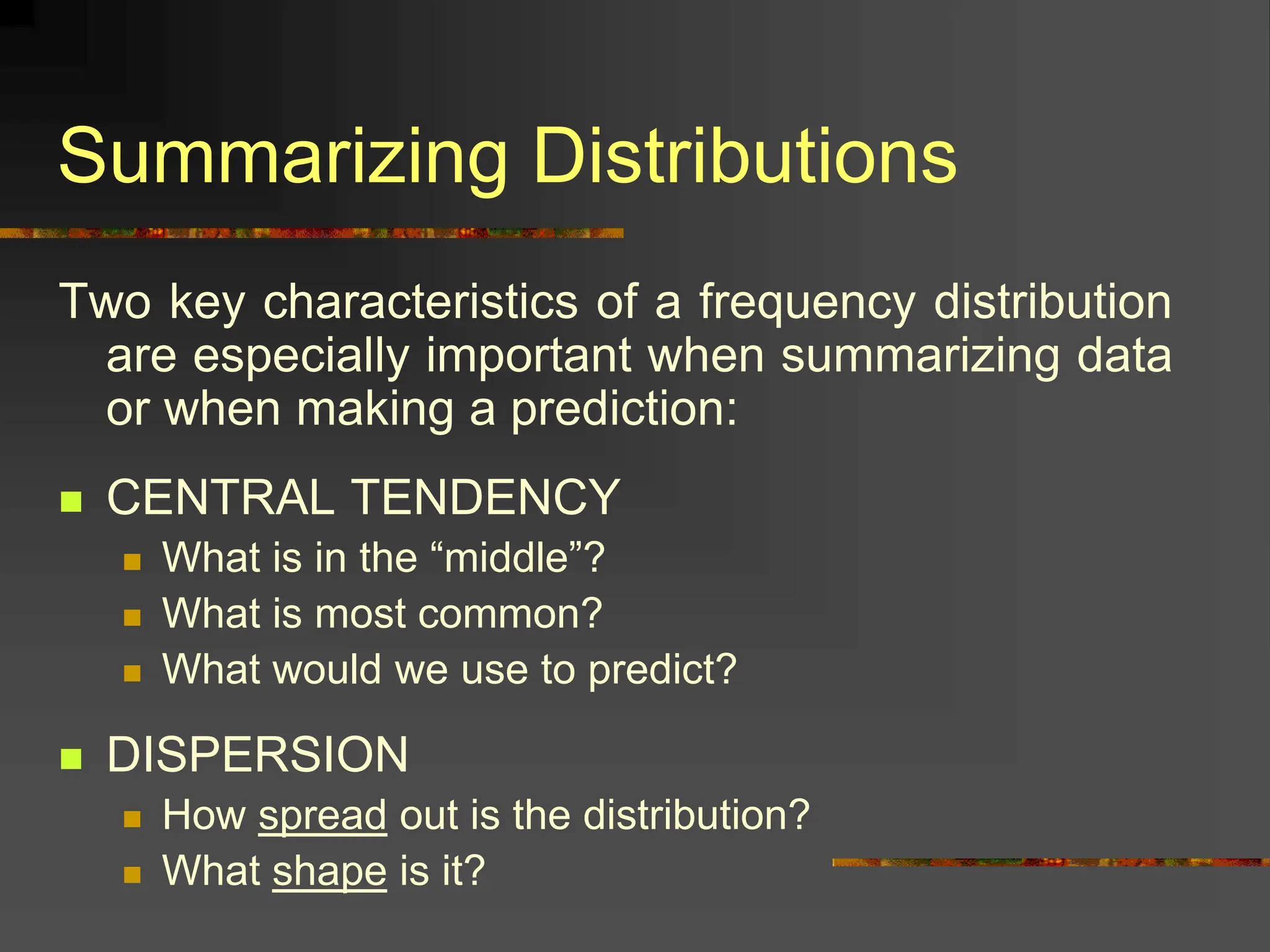
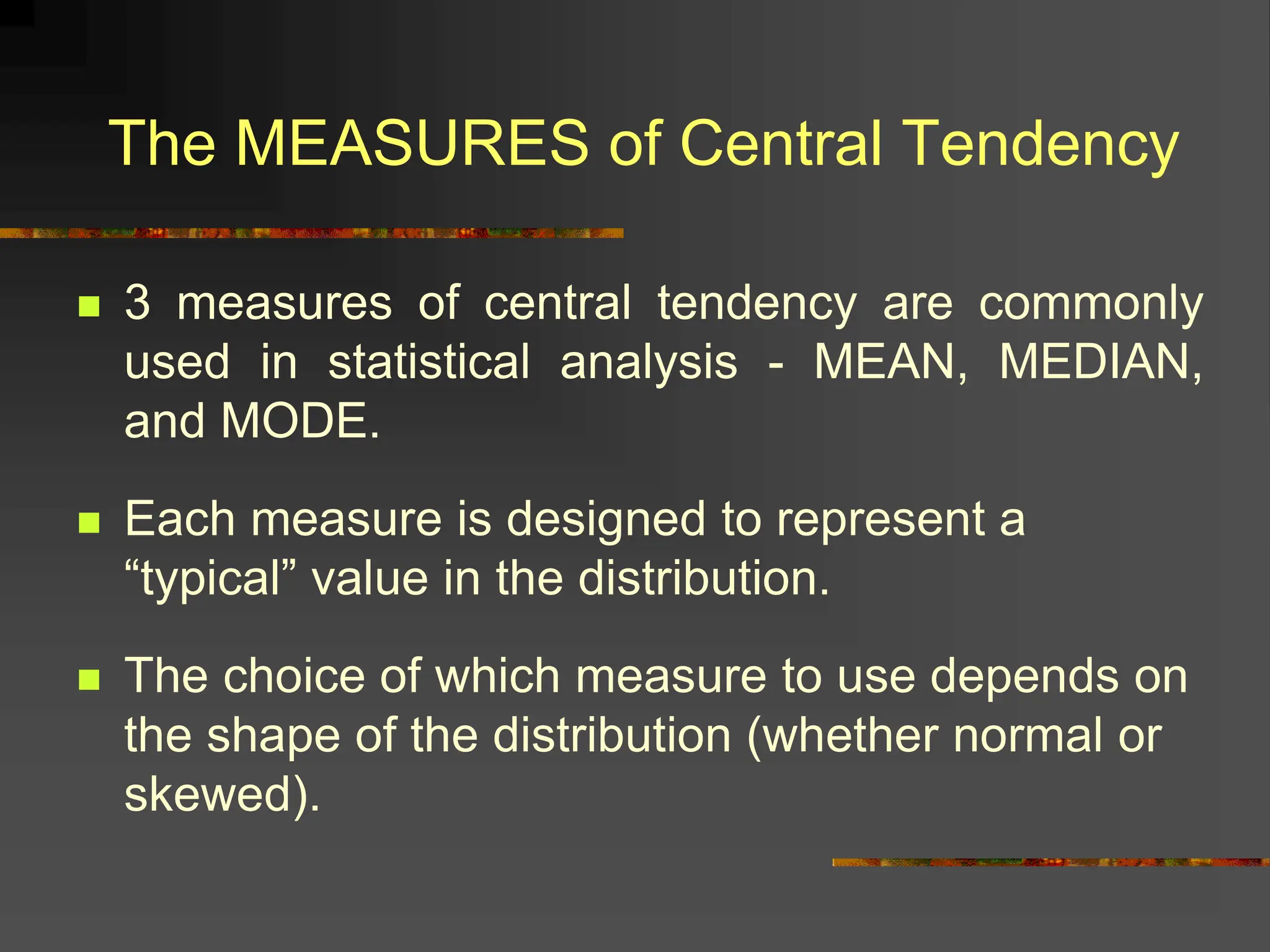
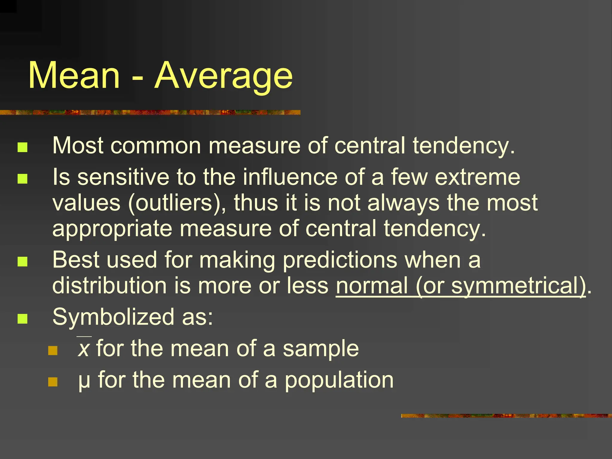
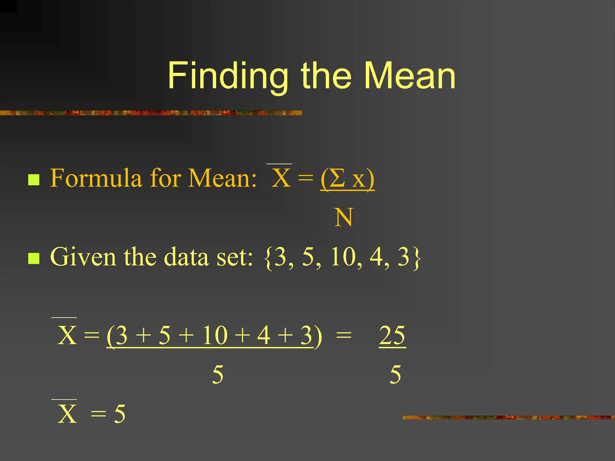
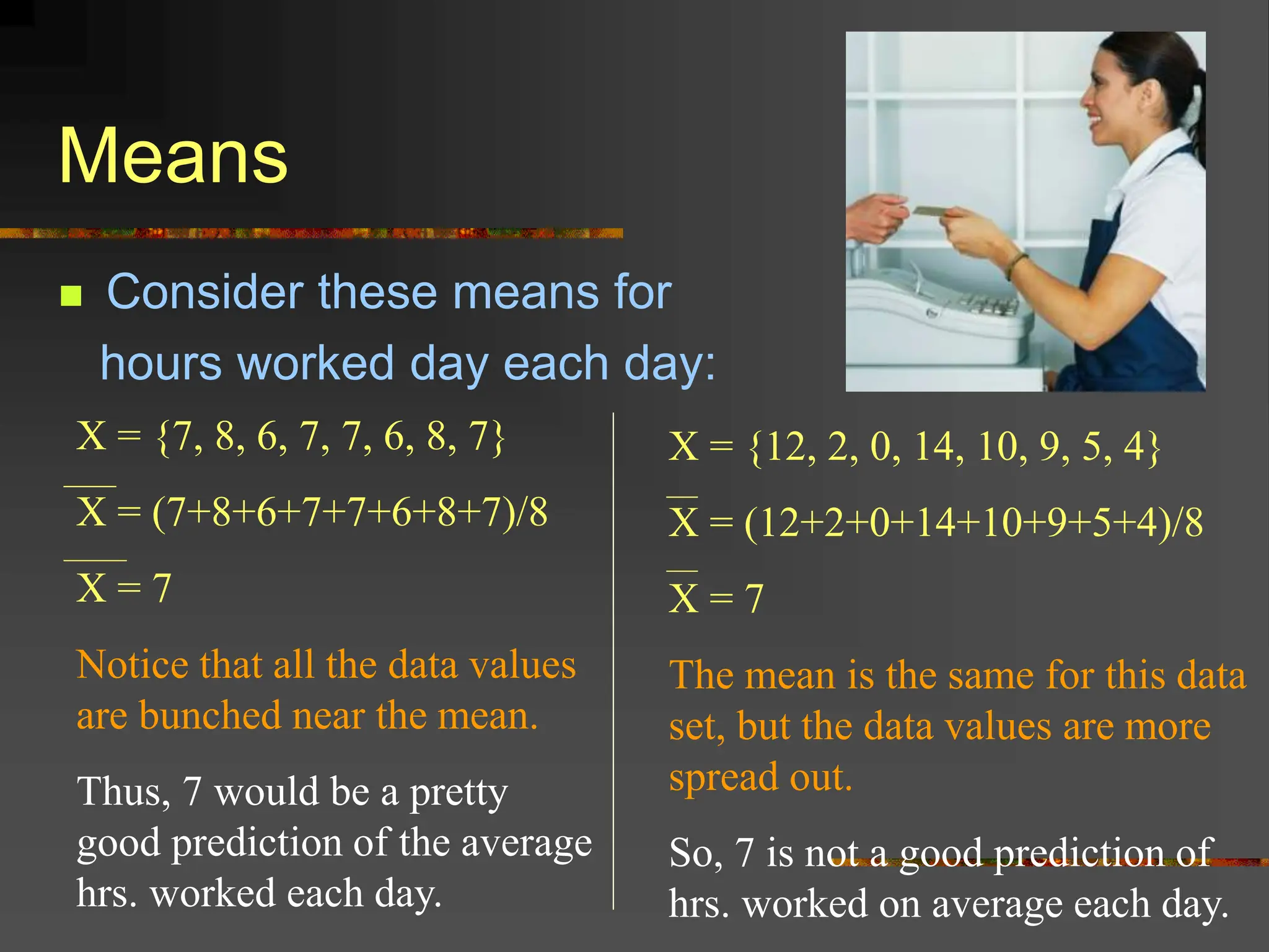
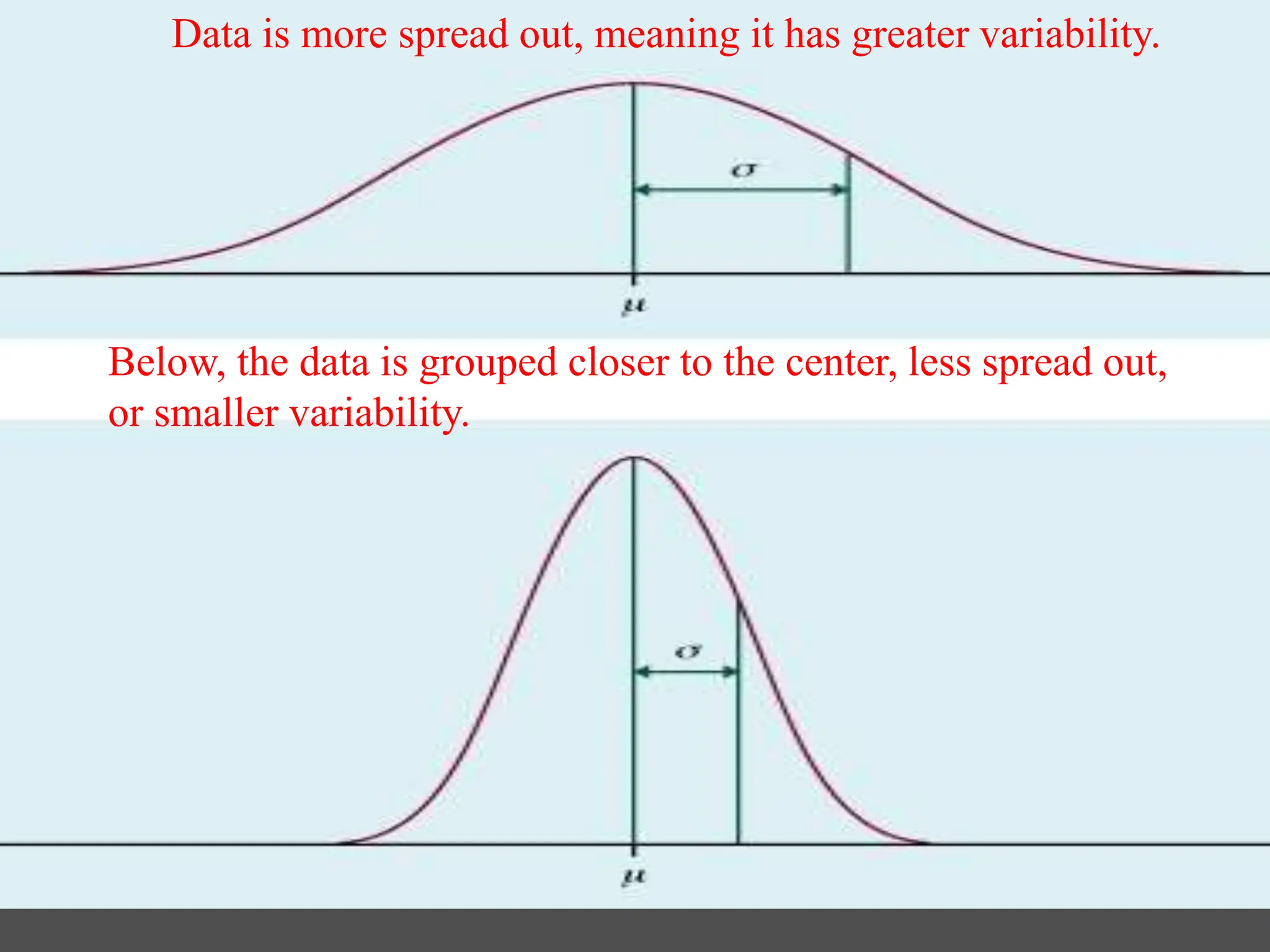
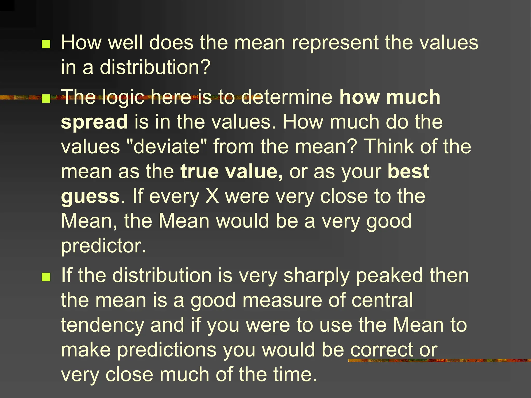
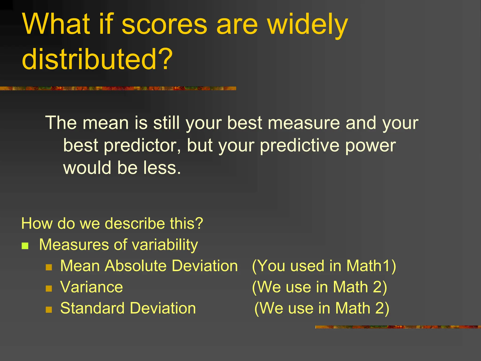
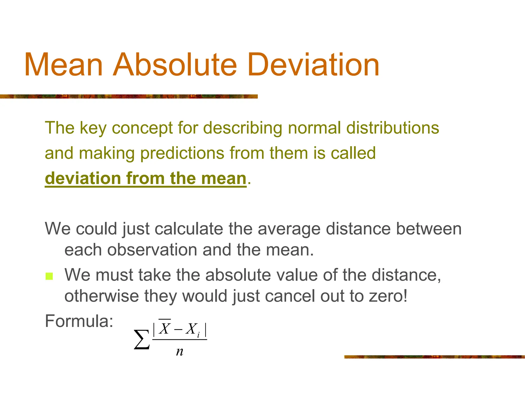
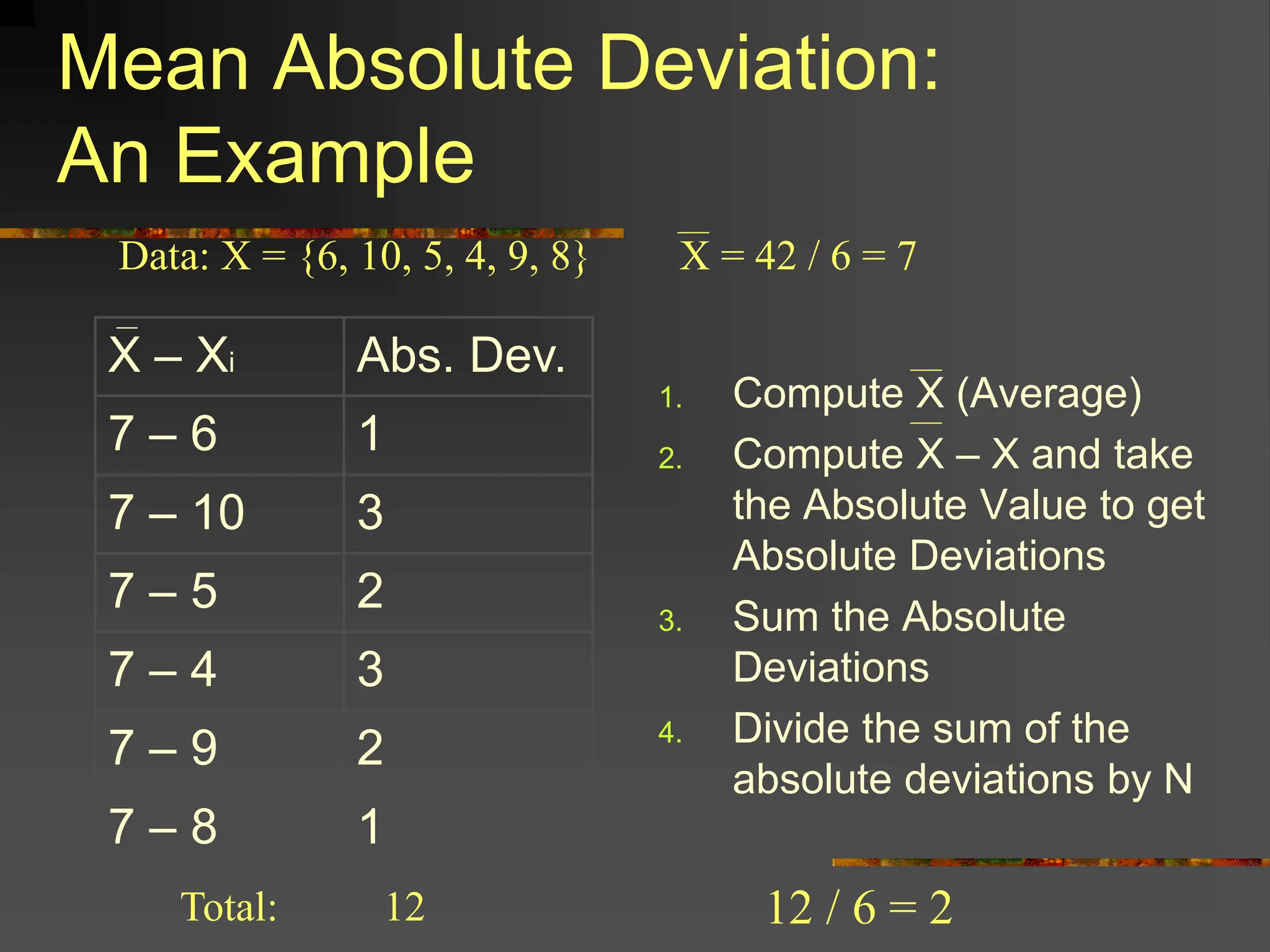
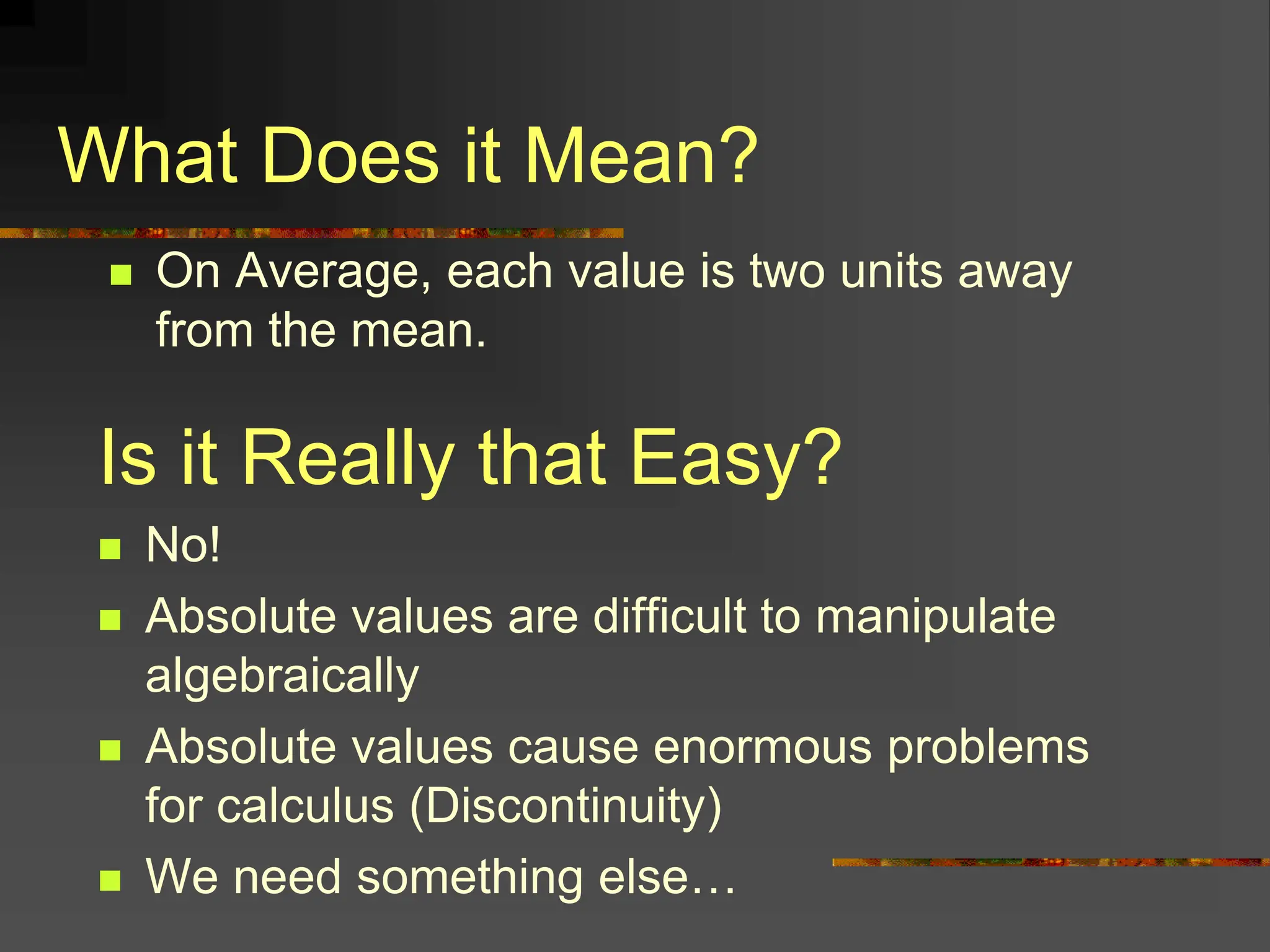
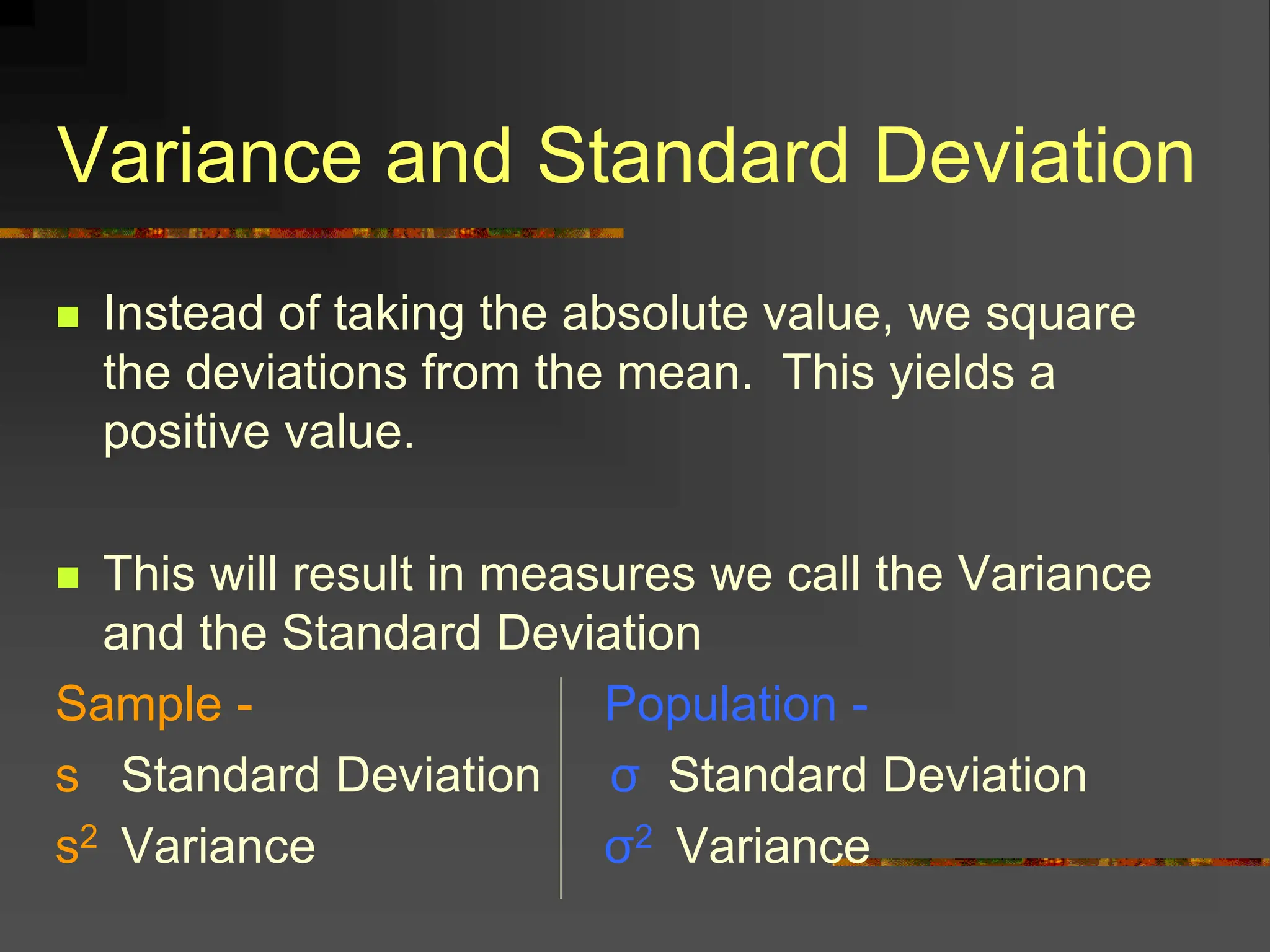
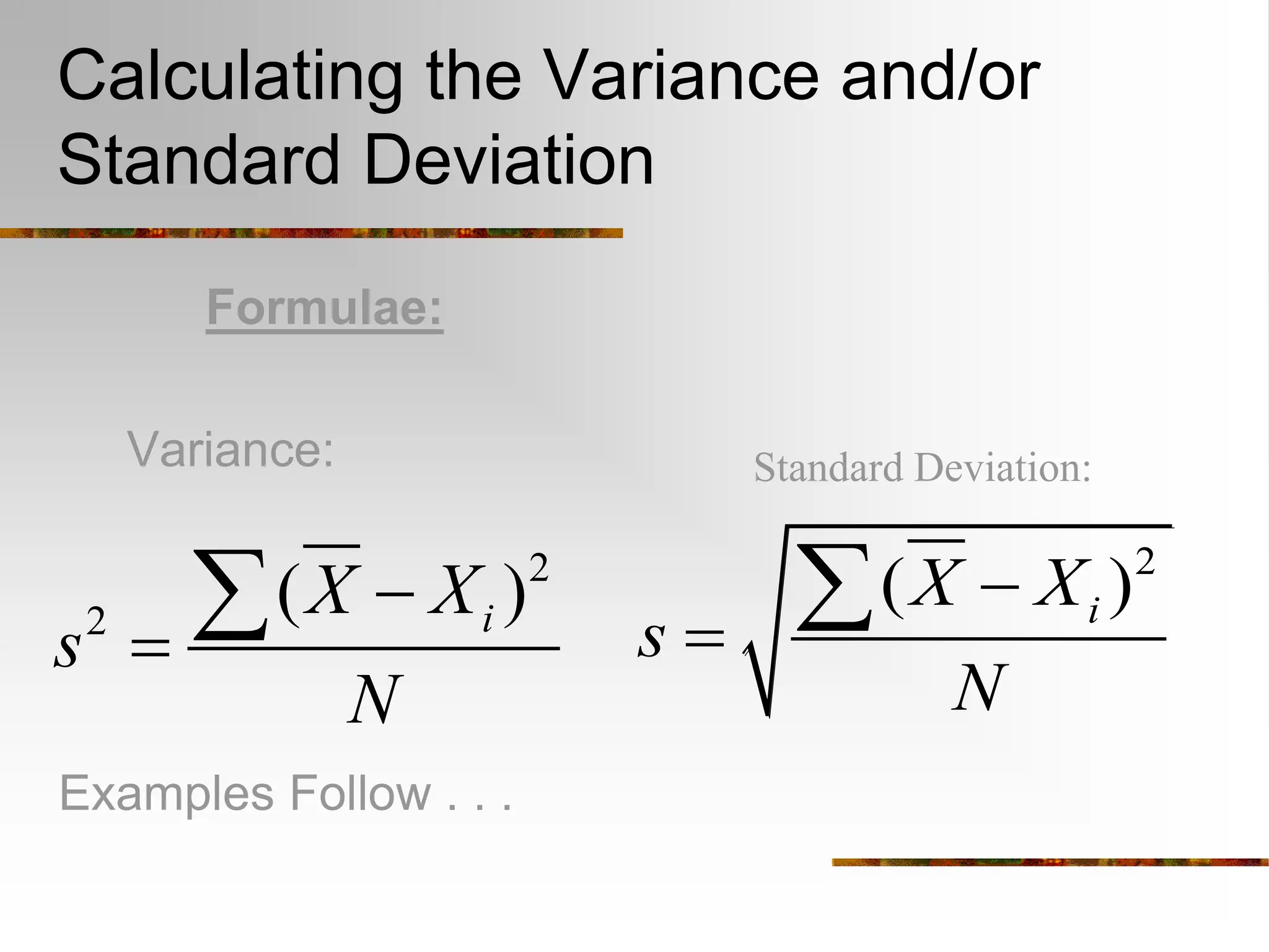
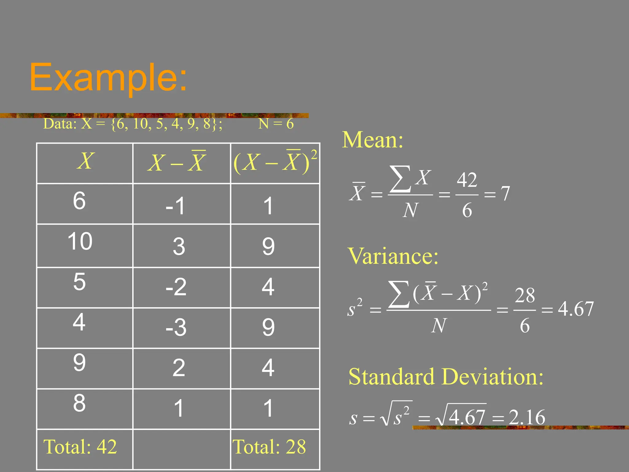
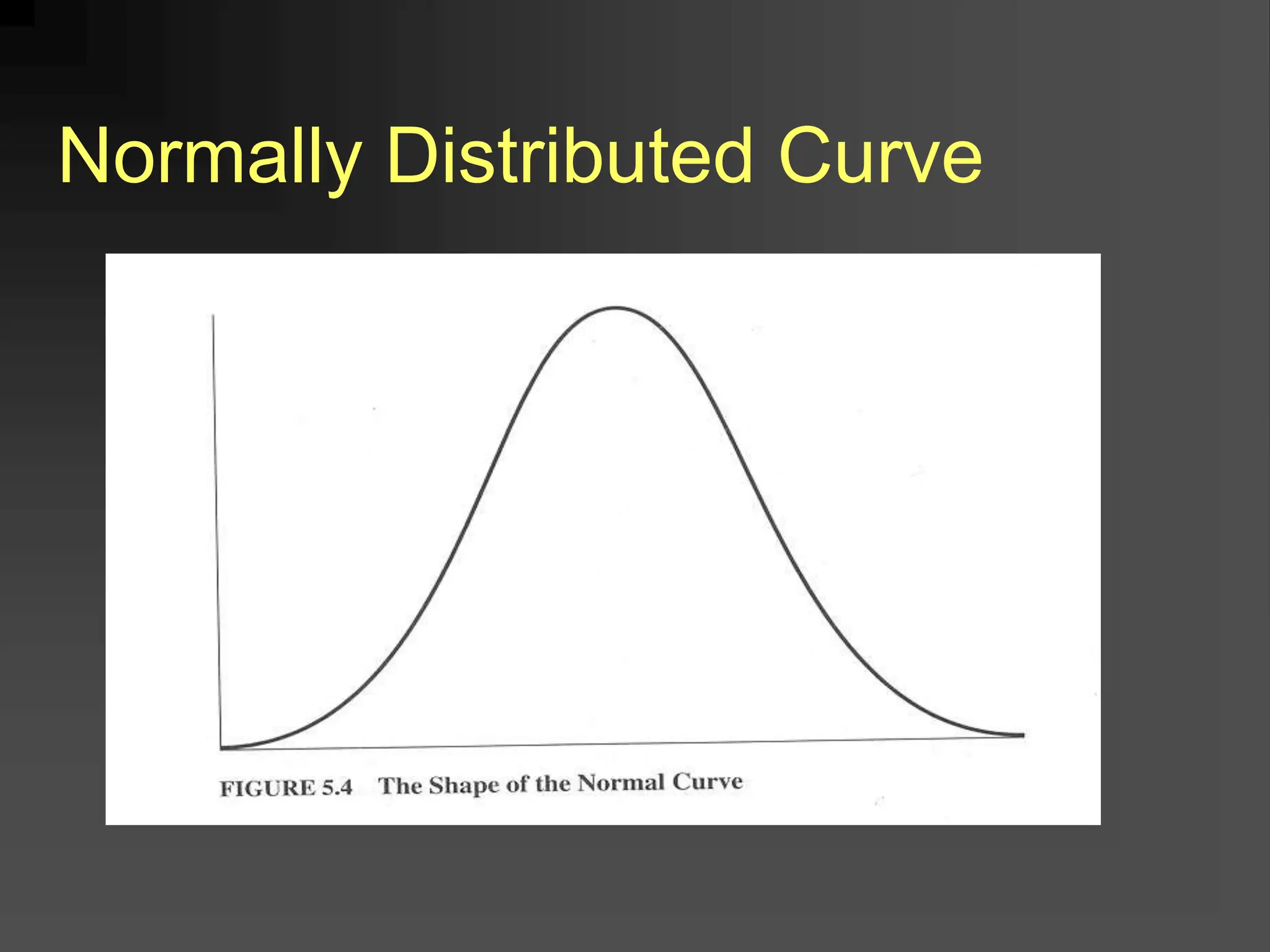
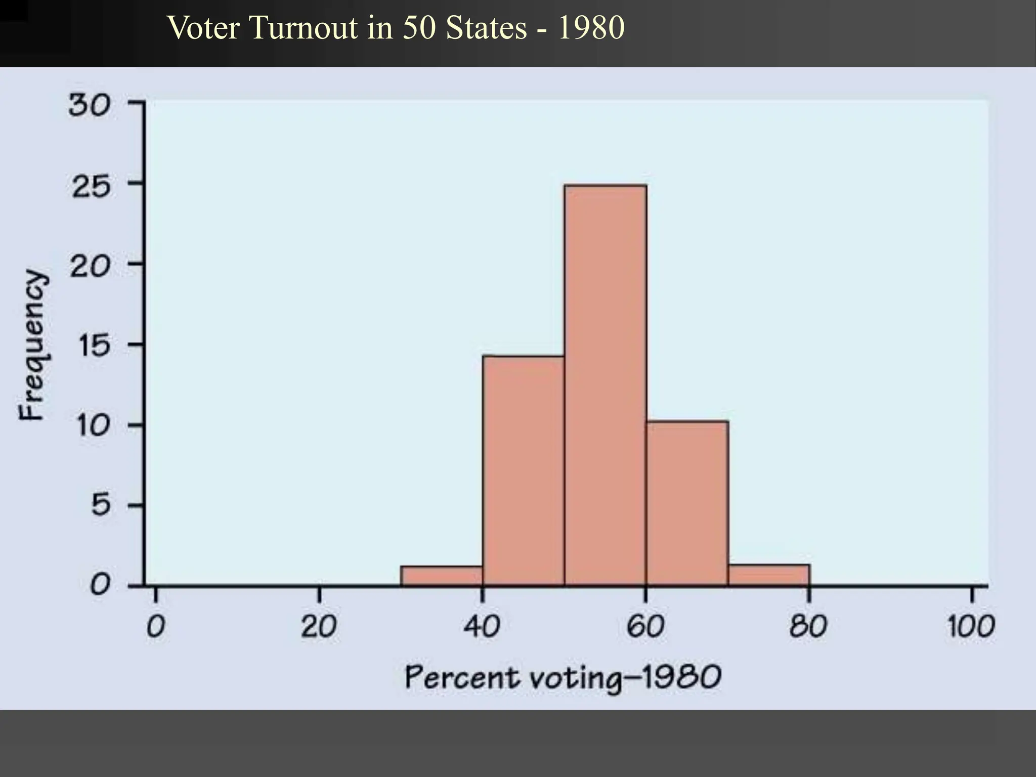
- The document discusses key concepts in descriptive statistics including types of distributions, measures of central tendency, and measures of dispersion. - It covers normal, skewed, and other types of distributions. Measures of central tendency discussed are mean, median, and mode. Measures of dispersion covered are variance and standard deviation. - The document uses examples and explanations to illustrate how to calculate and interpret these important statistical measures.

1. Central Tendency & Dispersion
 Types of Distributions: Normal, Skewed
 Central Tendency: Mean, Median, Mode
 Dispersion: Variance, Standard Deviation
This PowerPoint has been ripped off from I don’t know where,
and improved upon by yours truly…Mrs. T  Enjoy!

2. DESCRIPTIVE STATISTICS
are concerned with describing the
characteristics of frequency distributions
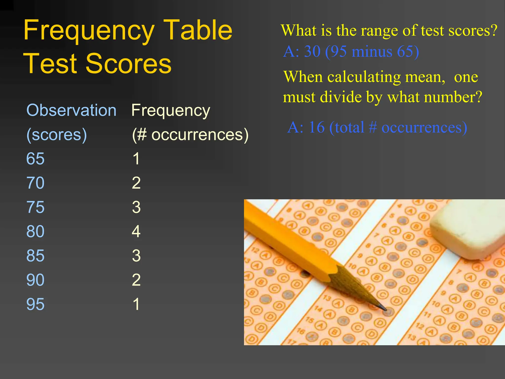
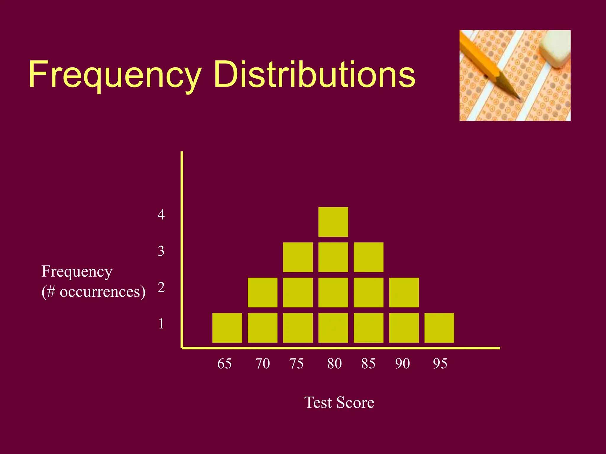
 Where is the center?
 What is the range?
 What is the shape [of the
distribution]?

3. Frequency Table
Test Scores
Observation Frequency
(scores) (# occurrences)
65 1
70 2
75 3
80 4
85 3
90 2
95 1
What is the range of test scores?
A: 30 (95 minus 65)
When calculating mean, one
must divide by what number?
A: 16 (total # occurrences)

4. Frequency Distributions
Test Score
Frequency
(# occurrences)
4
3
2
1
65 70 75 80 85 90 95

5. Normally Distributed Curve

6. Voter Turnout in 50 States - 1980

7. Skewed Distributions
We say the distribution is skewed
to the left  (when the “tail” is
to the left)
We say the distribution is skewed
to the right  (when the “tail” is
to the right)

8. Voter Turnout in 50 States - 1940
Q: Is this distribution, positively or negatively skewed?
Q: Would we say this distribution is
skewed to the left or right?
A: Negatively
A: Left (skewed in direction of tail)

9. Characteristics - Normal Distribution
 It is symmetrical - half the values are to one side of the
center (mean), and half the values are on the other side.
 The distribution is single-peaked, not bimodal or multi-
modal.
 Most of the data values will be “bunched” near the center
portion of the curve. As values become more extreme
they become less frequent with the “outliers” being found
at the “tails” of the distribution and are few in number.
 The Mean, Median, and Mode are the same in a perfectly
symmetrical normal distribution.
 Percentage of values that occur in any range of the curve
can be calculated using the Empirical Rule.

10. Empirical Rule

11. Summarizing Distributions
Two key characteristics of a frequency distribution
are especially important when summarizing data
or when making a prediction:
 CENTRAL TENDENCY
 What is in the “middle”?
 What is most common?
 What would we use to predict?
 DISPERSION
 How spread out is the distribution?
 What shape is it?

12.  3 measures of central tendency are commonly
used in statistical analysis - MEAN, MEDIAN,
and MODE.
 Each measure is designed to represent a
“typical” value in the distribution.
 The choice of which measure to use depends on
the shape of the distribution (whether normal or
skewed).
The MEASURES of Central Tendency

13. Mean - Average
 Most common measure of central tendency.
 Is sensitive to the influence of a few extreme
values (outliers), thus it is not always the most
appropriate measure of central tendency.
 Best used for making predictions when a
distribution is more or less normal (or symmetrical).
 Symbolized as:
 x for the mean of a sample
 μ for the mean of a population

14. Finding the Mean
 Formula for Mean: X = (Σ x)
N
 Given the data set: {3, 5, 10, 4, 3}
X = (3 + 5 + 10 + 4 + 3) = 25
5 5
X = 5

15. Find the Mean
Q: 85, 87, 89, 91, 98, 100
A: 91.67
Median: 90
Q: 5, 87, 89, 91, 98, 100
A: 78.3 (Extremely low score lowered the Mean)
Median: 90 (The median remained unchanged.)

16. Median
 Used to find middle value (center) of a distribution.
 Used when one must determine whether the data
values fall into either the upper 50% or lower 50%
of a distribution.
 Used when one needs to report the typical value of
a data set, ignoring the outliers (few extreme
values in a data set).
 Example: median salary, median home prices in a market
 Is a better indicator of central tendency than mean
when one has a skewed distribution.

17. To compute the median
 first you order the values of X from low to high:
 85, 90, 94, 94, 95, 97, 97, 97, 97, 98
 then count number of observations = 10.
 When the number of observations are even,
average the two middle numbers to calculate the
median.
 This example, 96 is the median
(middle) score.

18. Median
 Find the Median
4 5 6 6 7 8 9 10 12
 Find the Median
5 6 6 7 8 9 10 12
 Find the Median
5 6 6 7 8 9 10 100,000

19. Mode
 Used when the most typical (common) value is
desired.
 Often used with categorical data.
 The mode is not always unique. A distribution can
have no mode, one mode, or more than one mode.
When there are two modes, we say the distribution is
bimodal.
EXAMPLES:
a) {1,0,5,9,12,8} - No mode
b) {4,5,5,5,9,20,30} – mode = 5
c) {2,2,5,9,9,15} - bimodal, mode 2 and 9

20. Measures of Variability
 Central Tendency doesn’t tell us
everything Dispersion/Deviation/Spread
tells us a lot about how the data values
are distributed.
 We are most interested in:
Standard Deviation (σ) and
Variance (σ2)

21. Why can’t the mean tell us everything?
 Mean describes the average outcome.
 The question becomes how good a
representation of the distribution is the mean?
How good is the mean as a description of
central tendency -- or how accurate is the mean
as a predictor?
 ANSWER -- it depends on the shape of the
distribution. Is the distribution normal or
skewed?

22. Dispersion
 Once you determine that the data of interest is
normally distributed, ideally by producing a
histogram of the values, the next question to ask
is: How spread out are the values about the
mean?
 Dispersion is a key concept in statistical thinking.
 The basic question being asked is how much do
the values deviate from the Mean? The more
“bunched up” around the mean the better
your ability to make accurate predictions.

23. Means
 Consider these means for
hours worked day each day:
X = {7, 8, 6, 7, 7, 6, 8, 7}
X = (7+8+6+7+7+6+8+7)/8
X = 7
Notice that all the data values
are bunched near the mean.
Thus, 7 would be a pretty
good prediction of the average
hrs. worked each day.
X = {12, 2, 0, 14, 10, 9, 5, 4}
X = (12+2+0+14+10+9+5+4)/8
X = 7
The mean is the same for this data
set, but the data values are more
spread out.
So, 7 is not a good prediction of
hrs. worked on average each day.

24. Data is more spread out, meaning it has greater variability.
Below, the data is grouped closer to the center, less spread out,
or smaller variability.

25.  How well does the mean represent the values
in a distribution?
 The logic here is to determine how much
spread is in the values. How much do the
values "deviate" from the mean? Think of the
mean as the true value, or as your best
guess. If every X were very close to the
Mean, the Mean would be a very good
predictor.
 If the distribution is very sharply peaked then
the mean is a good measure of central
tendency and if you were to use the Mean to
make predictions you would be correct or
very close much of the time.

26. What if scores are widely
distributed?
The mean is still your best measure and your
best predictor, but your predictive power
would be less.
How do we describe this?
 Measures of variability
 Mean Absolute Deviation (You used in Math1)
 Variance (We use in Math 2)
 Standard Deviation (We use in Math 2)

27. Mean Absolute Deviation
The key concept for describing normal distributions
and making predictions from them is called
deviation from the mean.
We could just calculate the average distance between
each observation and the mean.
 We must take the absolute value of the distance,
otherwise they would just cancel out to zero!
Formula: | |
i
X X
n



28. Mean Absolute Deviation:
An Example
1. Compute X (Average)
2. Compute X – X and take
the Absolute Value to get
Absolute Deviations
3. Sum the Absolute
Deviations
4. Divide the sum of the
absolute deviations by N
X – Xi Abs. Dev.
7 – 6 1
7 – 10 3
7 – 5 2
7 – 4 3
7 – 9 2
7 – 8 1
Data: X = {6, 10, 5, 4, 9, 8} X = 42 / 6 = 7
Total: 12 12 / 6 = 2

29. What Does it Mean?
 On Average, each value is two units away
from the mean.
Is it Really that Easy?
 No!
 Absolute values are difficult to manipulate
algebraically
 Absolute values cause enormous problems
for calculus (Discontinuity)
 We need something else…

30. Variance and Standard Deviation
 Instead of taking the absolute value, we square
the deviations from the mean. This yields a
positive value.
 This will result in measures we call the Variance
and the Standard Deviation
Sample - Population -
s Standard Deviation σ Standard Deviation
s2 Variance σ2 Variance

31. Calculating the Variance and/or
Standard Deviation
Formulae:
Variance:
Examples Follow . . .
2
( )
i
X X
s
N



2
2
( )
i
X X
s
N



Standard Deviation:

32. Example:
-1 1
3 9
-2 4
-3 9
2 4
1 1
Data: X = {6, 10, 5, 4, 9, 8}; N = 6
Total: 42 Total: 28
Standard Deviation:
7
6
42




N
X
X
Mean:
Variance:
2
2
( ) 28
4.67
6
X X
s
N

  

16
.
2
67
.
4
2


 s
s
X
X  2
)
( X
X 
X
6
10
5
4
9
8