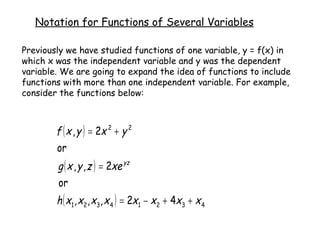
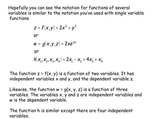
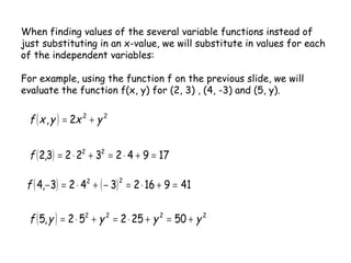
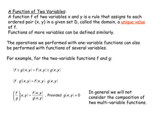
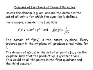
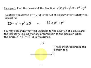
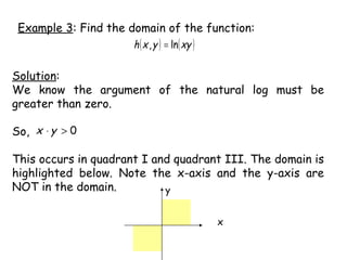
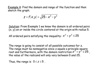
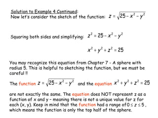
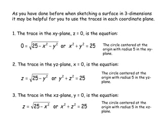
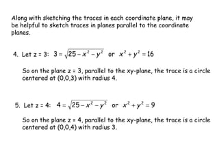
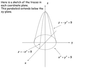
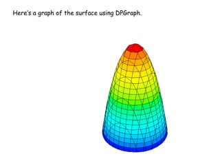
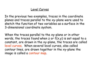
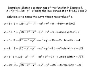
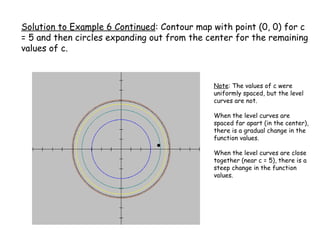
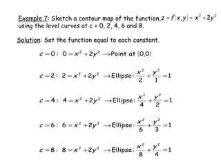
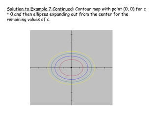
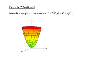
SlideShare a Scribd company logo
1 of 28
Download to read offline
Chapter 8: Functions of Several
Variables
Section 8.1
Introduction to Functions of Several Variables
Written by Karen Overman
Instructor of Mathematics
Tidewater Community College, Virginia Beach Campus
Virginia Beach, VA
With Assistance from a VCCS LearningWare Grant
In this lesson we will discuss:
o Notation of functions of several variables
o Domain of functions of several variables
o Graphs of functions of several variables
o Level curves for functions of several variables
Notation for Functions of Several Variables
Previously we have studied functions of one variable, y = f(x) in
which x was the independent variable and y was the dependent
variable. We are going to expand the idea of functions to include
functions with more than one independent variable. For example,
consider the functions below:
( )
( )
( ) 4
3
2
1
4
3
2
1
2
2
4
2
,
,
,
or
2
,
,
or
2
,
x
x
x
x
x
x
x
x
h
xe
z
y
x
g
y
x
y
x
f
yz
+
+
−
=
=
+
=
The function z = f(x, y) is a function of two variables. It has
independent variables x and y, and the dependent variable z.
Likewise, the function w = g(x, y, z) is a function of three
variables. The variables x, y and z are independent variables and
w is the dependent variable.
The function h is similar except there are four independent
variables.
Hopefully you can see the notation for functions of several
variables is similar to the notation you’ve used with single variable
functions.
( )
( )
( ) 4
3
2
1
4
3
2
1
2
2
4
2
,
,
,
or
2
,
,
or
2
,
x
x
x
x
x
x
x
x
h
xe
z
y
x
g
w
y
x
y
x
f
z
yz
+
+
−
=
=
=
+
=
=
When finding values of the several variable functions instead of
just substituting in an x-value, we will substitute in values for each
of the independent variables:
For example, using the function f on the previous slide, we will
evaluate the function f(x, y) for (2, 3) , (4, -3) and (5, y).
( )
( ) 17
9
4
2
3
2
2
3
,
2
2
,
2
2
2
2
=
+
⋅
=
+
⋅
=
+
=
f
y
x
y
x
f
( ) ( ) 41
9
16
2
3
4
2
3
,
4
2
2
=
+
⋅
=
−
+
⋅
=
−
f
( ) 2
2
2
2
50
25
2
5
2
,
5 y
y
y
y
f +
=
+
⋅
=
+
⋅
=
A Function of Two Variables:
A function f of two variables x and y is a rule that assigns to each
ordered pair (x, y) in a given set D, called the domain, a unique value
of f.
Functions of more variables can be defined similarly.
The operations we performed with one-variable functions can also
be performed with functions of several variables.
For example, for the two-variable functions f and g:
( )( ) ( ) ( )
( )( ) ( ) ( )
( ) ( )
( )
( ) 0
,
Provided
,
,
,
,
,
,
,
,
,
,
≠
=








⋅
=
⋅
±
=
±
y
x
g
y
x
g
y
x
f
y
x
g
f
y
x
g
y
x
f
y
x
g
f
y
x
g
y
x
f
y
x
g
f
In general we will not
consider the composition of
two multi-variable functions.
Domains of Functions of Several Variables:
Unless the domain is given, assume the domain is the
set of all points for which the equation is defined.
For example, consider the functions
( ) ( )
xy
y
x
g
y
x
y
x
f
1
,
and
3
, 2
2
=
+
=
The domain of f(x,y) is the entire xy-plane. Every
ordered pair in the xy-plane will produce a real value for
f.
The domain of g(x, y) is the set of all points (x, y) in the
xy-plane such that the product xy is greater than 0.
This would be all the points in the first quadrant and
the third quadrant.
Example 1: Find the domain of the function: ( ) 2
2
25
, y
x
y
x
f −
−
=
Solution: The domain of f(x, y) is the set of all points that satisfy the
inequality:
0
25 2
2
≥
−
− y
x
2
2
25 y
x +
≥
or
You may recognize that this is similar to the equation of a circle and
the inequality implies that any ordered pair on the circle or inside
the circle is in the domain.
25
2
2
=
+ y
x
x
y
The highlighted area is the
domain to f.
Example 2: Find the domain of the function:
( ) 16
,
, 2
2
2
−
+
+
= z
y
x
z
y
x
g
Solution:
Note that g is a function of three variables, so the domain is NOT an
area in the xy-plane. The domain of g is a solid in the 3-dimensional
coordinate system.
The expression under the radical must be nonnegative, resulting in
the inequality:
This implies that any ordered triple outside of the sphere centered
at the origin with radius 4 is in the domain.
16
or
0
16 2
2
2
2
2
2
≥
+
+
≥
−
+
+ z
y
x
z
y
x
Example 3: Find the domain of the function:
Solution:
We know the argument of the natural log must be
greater than zero.
So,
This occurs in quadrant I and quadrant III. The domain is
highlighted below. Note the x-axis and the y-axis are
NOT in the domain.
( ) ( )
xy
y
x
h ln
, =
0
>
⋅ y
x
x
y
Graphs of Functions of Several Variables
As you learned in 2-dimensional space the graph of a function can be
helpful to your understanding of the function. The graph gives an
illustration or visual representation of all the solutions to the
equation. We also want to use this tool with functions of two
variables.
The graph of a function of two variables, z = f(x, y), is the set of
ordered triples, (x, y, z) for which the ordered pair, (x, y) is in the
domain.
*The graph of z = f(x, y) is a surface in 3-dimensional space.
The graph of a function of three variables, w = f(x, y, z) is the set of
all points (x, y, z, w) for which the ordered triple, (x, y, z) is in the
domain.
*The graph of w = f(x, y, z) is in 4 dimensions.
We can’t draw this graph or the graphs of any functions with 3 or
more independent variables.
Example 4: Find the domain and range of the function and then
sketch the graph.
( ) 2
2
25
, y
x
y
x
f
z −
−
=
=
Solution: From Example 1 we know the domain is all ordered pairs
(x, y) on or inside the circle centered at the origin with radius 5.
All ordered pairs satisfying the inequality:
The range is going to consist of all possible outcomes for z.
The range must be nonnegative since z equals a principle square
root and furthermore, with the domain restriction: ,
the value of the radicand will only vary between 0 and 25.
Thus, the range is .
25
2
2
≤
+ y
x
5
0 ≤
≤ z
25
2
2
≤
+ y
x
25
2
2
2
=
+
+ z
y
x
2
2
2
25 y
x
z −
−
=
2
2
25 y
x
z −
−
=
Solution to Example 4 Continued:
Now let’s consider the sketch of the function:
Squaring both sides and simplifying:
You may recognize this equation from Chapter 7 - A sphere with
radius 5. This is helpful to sketching the function, but we must be
careful !!
The function and the equation
are not exactly the same. The equation does NOT represent z as a
function of x and y – meaning there is not a unique value for z for
each (x, y). Keep in mind that the function had a range of ,
which means the function is only the top half of the sphere.
2
2
25 y
x
z −
−
= 25
2
2
2
=
+
+ z
y
x
5
0 ≤
≤ z
As you have done before when sketching a surface in 3-dimensions
it may be helpful for you to use the traces in each coordinate plane.
1. The trace in the xy-plane, z = 0, is the equation:
25
or
25
0 2
2
2
2
=
+
−
−
= y
x
y
x The circle centered at the
origin with radius 5 in the xy-
plane.
2. The trace in the yz-plane, x = 0, is the equation:
25
or
25 2
2
2
=
+
−
= z
y
y
z
The circle centered at the
origin with radius 5 in the yz-
plane.
3. The trace in the xz-plane, y = 0, is the equation:
25
or
25 2
2
2
=
+
−
= z
x
x
z
The circle centered at the
origin with radius 5 in the xz-
plane.
Along with sketching the traces in each coordinate plane, it may
be helpful to sketch traces in planes parallel to the coordinate
planes.
4. Let z = 3: 16
or
25
3 2
2
2
2
=
+
−
−
= y
x
y
x
So on the plane z = 3, parallel to the xy-plane, the trace is a circle
centered at (0,0,3) with radius 4.
5. Let z = 4: 9
or
25
4 2
2
2
2
=
+
−
−
= y
x
y
x
So on the plane z = 4, parallel to the xy-plane, the trace is a circle
centered at (0,0,4) with radius 3.
Here is a SKETCH with the three traces in the coordinate planes
and the additional two traces in planes parallel to the xy-plane.
Keep in mind that this is just a sketch. It is giving you a rough
idea of what the function looks like. It may also be helpful to use
a 3-dimensional graphing utility to get a better picture.
z = 3
z = 4
Here is a graph of the function using the 3-dimensional
graphing utility DPGraph.
x
y
z
Example 5: Sketch the surface:
2
2
9 y
x
z −
−
=
Solution: The domain is the entire xy-plane and the range is .
1. The trace in the xy-plane, z = 0, is the equation:
2. The trace in the yz-plane, x = 0, is the equation:
3. The trace in the xz-plane, y = 0, is the equation:
9
2
2
=
+ y
x Circle
9
2
+
−
= y
z Parabola
9
2
+
−
= x
z Parabola
9
≤
z
Solution to Example 5 Continued:
Traces parallel to the xy-plane include the following two.
4. The trace in the plane, z = 5, is the equation:
5. The trace in the plane, z = -7, is the equation:
4
or
9
5
2
2
2
2
=
+
−
−
=
y
x
y
x
Circle centered at (0, 0, 5) with
radius 2.
16
or
9
7
2
2
2
2
=
+
−
−
=
−
y
x
y
x
Circle centered at (0, 0, -7) with
radius 4.
x
y
z
9
2
2
=
+ y
x
9
2
+
−
= y
z
9
2
+
−
= x
z
Here is a sketch of the traces in
each coordinate plane.
This paraboloid extends below the
xy-plane.
Here’s a graph of the surface using DPGraph.
In the previous two examples, traces in the coordinate
planes and traces parallel to the xy-plane were used to
sketch the function of two variables as a surface in the
3-dimensional coordinate system.
When the traces parallel to the xy-plane or in other
words, the traces found when z or f(x,y) is set equal to a
constant, are drawn in the xy-plane, the traces are called
level curves. When several level curves, also called
contour lines, are drawn together in the xy-plane the
image is called a contour map.
Level Curves
Example 6: Sketch a contour map of the function in Example 4,
using the level curves at c = 5,4,3,2,1 and 0.
Solution: c = a means the curve when z has a value of a.
( )
5
r
with
Circle
25
y
x
25
0
:
0
24
r
with
Circle
24
y
x
25
1
:
1
21
r
with
Circle
21
y
x
25
2
:
2
4
r
with
Circle
16
y
x
25
3
:
3
3
r
with
Circle
9
y
x
25
4
:
4
0
,
0
at
Point
0
y
x
25
5
:
5
2
2
2
2
2
2
2
2
2
2
2
2
2
2
2
2
2
2
2
2
2
2
2
2
=
→
=
+
→
−
−
=
=
=
→
=
+
→
−
−
=
=
=
→
=
+
→
−
−
=
=
=
→
=
+
→
−
−
=
=
=
→
=
+
→
−
−
=
=
→
=
+
→
−
−
=
=
y
x
c
y
x
c
y
x
c
y
x
c
y
x
c
y
x
c
( ) 2
2
25
, y
x
y
x
f
z −
−
=
=
Solution to Example 6 Continued: Contour map with point (0, 0) for c
= 5 and then circles expanding out from the center for the remaining
values of c.
Note: The values of c were
uniformly spaced, but the level
curves are not.
When the level curves are
spaced far apart (in the center),
there is a gradual change in the
function values.
When the level curves are close
together (near c = 5), there is a
steep change in the function
values.
Example 7: Sketch a contour map of the function,
using the level curves at c = 0, 2, 4, 6 and 8.
( ) 2
2
2
, y
x
y
x
f
z +
=
=
Solution: Set the function equal to each constant.
( )
1
4
8
:
Ellipse
2
8
:
8
1
3
6
:
Ellipse
2
6
:
6
1
2
4
:
Ellipse
2
4
:
4
1
1
2
:
Ellipse
2
2
:
2
0
,
0
at
Point
2
0
:
0
2
2
2
2
2
2
2
2
2
2
2
2
2
2
2
2
2
2
=
+
→
+
=
=
=
+
→
+
=
=
=
+
→
+
=
=
=
+
→
+
=
=
→
+
=
=
y
x
y
x
c
y
x
y
x
c
y
x
y
x
c
y
x
y
x
c
y
x
c
Solution to Example 7 Continued: Contour map with point (0, 0) for c
= 0 and then ellipses expanding out from the center for the
remaining values of c.
Example 7 Continued:
Here is a graph of the surface .
( ) 2
2
2
, y
x
y
x
f
z +
=
=
Note:
3. Sketching functions of two variables in 3-dimensions is
challenging and will take quite a bit of practice. Using the
traces and level curves can be extremely beneficial.
In the beginning, using 3-dimensional graphing utility will help
you visualize the surfaces and see how the traces and level
curves relate.
2. The idea of a level curve can be extended to functions of
three variables. If w = g(x, y, z) is a function of three
variables and k is a constant, then g(x, y, z) = k is considered a
level surface of the function g. Though we may be able to
draw the level surface, we still cannot draw the function g in 4
dimensions.

More Related Content

Similar to Functions of several variables.pdf

Module 3 quadratic functions
Module 3   quadratic functionsModule 3   quadratic functions
Module 3 quadratic functionsdionesioable
 
Quadraticfunctionpresentation 100127142417-phpapp02
Quadraticfunctionpresentation 100127142417-phpapp02Quadraticfunctionpresentation 100127142417-phpapp02
Quadraticfunctionpresentation 100127142417-phpapp02Vine Gonzales
 
Solution 3
Solution 3Solution 3
Solution 3aldrins
 
Calculusseveralvariables.ppt
Calculusseveralvariables.pptCalculusseveralvariables.ppt
Calculusseveralvariables.pptssuser055963
 
Introduction to Functions
Introduction to FunctionsIntroduction to Functions
Introduction to FunctionsMelanie Loslo
 
Module 2 lesson 4 notes
Module 2 lesson 4 notesModule 2 lesson 4 notes
Module 2 lesson 4 notestoni dimella
 
Mathematics 3.pdf civil engineering concrete
Mathematics 3.pdf civil engineering concreteMathematics 3.pdf civil engineering concrete
Mathematics 3.pdf civil engineering concretemocr84810
 
Chapter3partialderivatives 150105021210-conversion-gate02
Chapter3partialderivatives 150105021210-conversion-gate02Chapter3partialderivatives 150105021210-conversion-gate02
Chapter3partialderivatives 150105021210-conversion-gate02Cleophas Rwemera
 
Applied Calculus Chapter 3 partial derivatives
Applied Calculus Chapter  3 partial derivativesApplied Calculus Chapter  3 partial derivatives
Applied Calculus Chapter 3 partial derivativesJ C
 
Modeling with Quadratics
Modeling with QuadraticsModeling with Quadratics
Modeling with QuadraticsPLeach
 
Module 2 linear functions
Module 2   linear functionsModule 2   linear functions
Module 2 linear functionsdionesioable
 
Partial differentiation B tech
Partial differentiation B techPartial differentiation B tech
Partial differentiation B techRaj verma
 
Solution 3
Solution 3Solution 3
Solution 3aldrins
 
Assignment For Matlab Report Subject Calculus 2
Assignment For Matlab Report Subject  Calculus 2Assignment For Matlab Report Subject  Calculus 2
Assignment For Matlab Report Subject Calculus 2Laurie Smith
 
Module 3 exponential and logarithmic functions
Module 3   exponential and logarithmic functionsModule 3   exponential and logarithmic functions
Module 3 exponential and logarithmic functionsdionesioable
 

Similar to Functions of several variables.pdf (20)

Grph quad fncts
Grph quad fnctsGrph quad fncts
Grph quad fncts
 
exponen dan logaritma
exponen dan logaritmaexponen dan logaritma
exponen dan logaritma
 
Functions
FunctionsFunctions
Functions
 
Module 3 quadratic functions
Module 3   quadratic functionsModule 3   quadratic functions
Module 3 quadratic functions
 
mc-ty-polynomial-2009-1.pdf
mc-ty-polynomial-2009-1.pdfmc-ty-polynomial-2009-1.pdf
mc-ty-polynomial-2009-1.pdf
 
Quadraticfunctionpresentation 100127142417-phpapp02
Quadraticfunctionpresentation 100127142417-phpapp02Quadraticfunctionpresentation 100127142417-phpapp02
Quadraticfunctionpresentation 100127142417-phpapp02
 
Solution 3
Solution 3Solution 3
Solution 3
 
Calculusseveralvariables.ppt
Calculusseveralvariables.pptCalculusseveralvariables.ppt
Calculusseveralvariables.ppt
 
Introduction to Functions
Introduction to FunctionsIntroduction to Functions
Introduction to Functions
 
Module 2 lesson 4 notes
Module 2 lesson 4 notesModule 2 lesson 4 notes
Module 2 lesson 4 notes
 
Mathematics 3.pdf civil engineering concrete
Mathematics 3.pdf civil engineering concreteMathematics 3.pdf civil engineering concrete
Mathematics 3.pdf civil engineering concrete
 
Chapter3partialderivatives 150105021210-conversion-gate02
Chapter3partialderivatives 150105021210-conversion-gate02Chapter3partialderivatives 150105021210-conversion-gate02
Chapter3partialderivatives 150105021210-conversion-gate02
 
Applied Calculus Chapter 3 partial derivatives
Applied Calculus Chapter  3 partial derivativesApplied Calculus Chapter  3 partial derivatives
Applied Calculus Chapter 3 partial derivatives
 
Modeling with Quadratics
Modeling with QuadraticsModeling with Quadratics
Modeling with Quadratics
 
Module 2 linear functions
Module 2   linear functionsModule 2   linear functions
Module 2 linear functions
 
Partial differentiation B tech
Partial differentiation B techPartial differentiation B tech
Partial differentiation B tech
 
Solution 3
Solution 3Solution 3
Solution 3
 
R lecture co4_math 21-1
R lecture co4_math 21-1R lecture co4_math 21-1
R lecture co4_math 21-1
 
Assignment For Matlab Report Subject Calculus 2
Assignment For Matlab Report Subject  Calculus 2Assignment For Matlab Report Subject  Calculus 2
Assignment For Matlab Report Subject Calculus 2
 
Module 3 exponential and logarithmic functions
Module 3   exponential and logarithmic functionsModule 3   exponential and logarithmic functions
Module 3 exponential and logarithmic functions
 

Recently uploaded

DeepFakes presentation : brief idea of DeepFakes
DeepFakes presentation : brief idea of DeepFakesDeepFakes presentation : brief idea of DeepFakes
DeepFakes presentation : brief idea of DeepFakesMayuraD1
 
Employee leave management system project.
Employee leave management system project.Employee leave management system project.
Employee leave management system project.Kamal Acharya
 
💚Trustworthy Call Girls Pune Call Girls Service Just Call 🍑👄6378878445 🍑👄 Top...
💚Trustworthy Call Girls Pune Call Girls Service Just Call 🍑👄6378878445 🍑👄 Top...💚Trustworthy Call Girls Pune Call Girls Service Just Call 🍑👄6378878445 🍑👄 Top...
💚Trustworthy Call Girls Pune Call Girls Service Just Call 🍑👄6378878445 🍑👄 Top...vershagrag
 
Tamil Call Girls Bhayandar WhatsApp +91-9930687706, Best Service
Tamil Call Girls Bhayandar WhatsApp +91-9930687706, Best ServiceTamil Call Girls Bhayandar WhatsApp +91-9930687706, Best Service
Tamil Call Girls Bhayandar WhatsApp +91-9930687706, Best Servicemeghakumariji156
 
Introduction to Data Visualization,Matplotlib.pdf
Introduction to Data Visualization,Matplotlib.pdfIntroduction to Data Visualization,Matplotlib.pdf
Introduction to Data Visualization,Matplotlib.pdfsumitt6_25730773
 
1_Introduction + EAM Vocabulary + how to navigate in EAM.pdf
1_Introduction + EAM Vocabulary + how to navigate in EAM.pdf1_Introduction + EAM Vocabulary + how to navigate in EAM.pdf
1_Introduction + EAM Vocabulary + how to navigate in EAM.pdfAldoGarca30
 
Introduction to Serverless with AWS Lambda
Introduction to Serverless with AWS LambdaIntroduction to Serverless with AWS Lambda
Introduction to Serverless with AWS LambdaOmar Fathy
 
Work-Permit-Receiver-in-Saudi-Aramco.pptx
Work-Permit-Receiver-in-Saudi-Aramco.pptxWork-Permit-Receiver-in-Saudi-Aramco.pptx
Work-Permit-Receiver-in-Saudi-Aramco.pptxJuliansyahHarahap1
 
Double Revolving field theory-how the rotor develops torque
Double Revolving field theory-how the rotor develops torqueDouble Revolving field theory-how the rotor develops torque
Double Revolving field theory-how the rotor develops torqueBhangaleSonal
 
Generative AI or GenAI technology based PPT
Generative AI or GenAI technology based PPTGenerative AI or GenAI technology based PPT
Generative AI or GenAI technology based PPTbhaskargani46
 
Hostel management system project report..pdf
Hostel management system project report..pdfHostel management system project report..pdf
Hostel management system project report..pdfKamal Acharya
 
"Lesotho Leaps Forward: A Chronicle of Transformative Developments"
"Lesotho Leaps Forward: A Chronicle of Transformative Developments""Lesotho Leaps Forward: A Chronicle of Transformative Developments"
"Lesotho Leaps Forward: A Chronicle of Transformative Developments"mphochane1998
 
Computer Networks Basics of Network Devices
Computer Networks  Basics of Network DevicesComputer Networks  Basics of Network Devices
Computer Networks Basics of Network DevicesChandrakantDivate1
 
HAND TOOLS USED AT ELECTRONICS WORK PRESENTED BY KOUSTAV SARKAR
HAND TOOLS USED AT ELECTRONICS WORK PRESENTED BY KOUSTAV SARKARHAND TOOLS USED AT ELECTRONICS WORK PRESENTED BY KOUSTAV SARKAR
HAND TOOLS USED AT ELECTRONICS WORK PRESENTED BY KOUSTAV SARKARKOUSTAV SARKAR
 
A CASE STUDY ON CERAMIC INDUSTRY OF BANGLADESH.pptx
A CASE STUDY ON CERAMIC INDUSTRY OF BANGLADESH.pptxA CASE STUDY ON CERAMIC INDUSTRY OF BANGLADESH.pptx
A CASE STUDY ON CERAMIC INDUSTRY OF BANGLADESH.pptxmaisarahman1
 
S1S2 B.Arch MGU - HOA1&2 Module 3 -Temple Architecture of Kerala.pptx
S1S2 B.Arch MGU - HOA1&2 Module 3 -Temple Architecture of Kerala.pptxS1S2 B.Arch MGU - HOA1&2 Module 3 -Temple Architecture of Kerala.pptx
S1S2 B.Arch MGU - HOA1&2 Module 3 -Temple Architecture of Kerala.pptxSCMS School of Architecture
 
DC MACHINE-Motoring and generation, Armature circuit equation
DC MACHINE-Motoring and generation, Armature circuit equationDC MACHINE-Motoring and generation, Armature circuit equation
DC MACHINE-Motoring and generation, Armature circuit equationBhangaleSonal
 
Digital Communication Essentials: DPCM, DM, and ADM .pptx
Digital Communication Essentials: DPCM, DM, and ADM .pptxDigital Communication Essentials: DPCM, DM, and ADM .pptx
Digital Communication Essentials: DPCM, DM, and ADM .pptxpritamlangde
 
Thermal Engineering -unit - III & IV.ppt
Thermal Engineering -unit - III & IV.pptThermal Engineering -unit - III & IV.ppt
Thermal Engineering -unit - III & IV.pptDineshKumar4165
 

Recently uploaded (20)

DeepFakes presentation : brief idea of DeepFakes
DeepFakes presentation : brief idea of DeepFakesDeepFakes presentation : brief idea of DeepFakes
DeepFakes presentation : brief idea of DeepFakes
 
Employee leave management system project.
Employee leave management system project.Employee leave management system project.
Employee leave management system project.
 
💚Trustworthy Call Girls Pune Call Girls Service Just Call 🍑👄6378878445 🍑👄 Top...
💚Trustworthy Call Girls Pune Call Girls Service Just Call 🍑👄6378878445 🍑👄 Top...💚Trustworthy Call Girls Pune Call Girls Service Just Call 🍑👄6378878445 🍑👄 Top...
💚Trustworthy Call Girls Pune Call Girls Service Just Call 🍑👄6378878445 🍑👄 Top...
 
Tamil Call Girls Bhayandar WhatsApp +91-9930687706, Best Service
Tamil Call Girls Bhayandar WhatsApp +91-9930687706, Best ServiceTamil Call Girls Bhayandar WhatsApp +91-9930687706, Best Service
Tamil Call Girls Bhayandar WhatsApp +91-9930687706, Best Service
 
Introduction to Data Visualization,Matplotlib.pdf
Introduction to Data Visualization,Matplotlib.pdfIntroduction to Data Visualization,Matplotlib.pdf
Introduction to Data Visualization,Matplotlib.pdf
 
1_Introduction + EAM Vocabulary + how to navigate in EAM.pdf
1_Introduction + EAM Vocabulary + how to navigate in EAM.pdf1_Introduction + EAM Vocabulary + how to navigate in EAM.pdf
1_Introduction + EAM Vocabulary + how to navigate in EAM.pdf
 
Introduction to Serverless with AWS Lambda
Introduction to Serverless with AWS LambdaIntroduction to Serverless with AWS Lambda
Introduction to Serverless with AWS Lambda
 
Work-Permit-Receiver-in-Saudi-Aramco.pptx
Work-Permit-Receiver-in-Saudi-Aramco.pptxWork-Permit-Receiver-in-Saudi-Aramco.pptx
Work-Permit-Receiver-in-Saudi-Aramco.pptx
 
Double Revolving field theory-how the rotor develops torque
Double Revolving field theory-how the rotor develops torqueDouble Revolving field theory-how the rotor develops torque
Double Revolving field theory-how the rotor develops torque
 
Generative AI or GenAI technology based PPT
Generative AI or GenAI technology based PPTGenerative AI or GenAI technology based PPT
Generative AI or GenAI technology based PPT
 
Hostel management system project report..pdf
Hostel management system project report..pdfHostel management system project report..pdf
Hostel management system project report..pdf
 
"Lesotho Leaps Forward: A Chronicle of Transformative Developments"
"Lesotho Leaps Forward: A Chronicle of Transformative Developments""Lesotho Leaps Forward: A Chronicle of Transformative Developments"
"Lesotho Leaps Forward: A Chronicle of Transformative Developments"
 
Computer Networks Basics of Network Devices
Computer Networks  Basics of Network DevicesComputer Networks  Basics of Network Devices
Computer Networks Basics of Network Devices
 
Integrated Test Rig For HTFE-25 - Neometrix
Integrated Test Rig For HTFE-25 - NeometrixIntegrated Test Rig For HTFE-25 - Neometrix
Integrated Test Rig For HTFE-25 - Neometrix
 
HAND TOOLS USED AT ELECTRONICS WORK PRESENTED BY KOUSTAV SARKAR
HAND TOOLS USED AT ELECTRONICS WORK PRESENTED BY KOUSTAV SARKARHAND TOOLS USED AT ELECTRONICS WORK PRESENTED BY KOUSTAV SARKAR
HAND TOOLS USED AT ELECTRONICS WORK PRESENTED BY KOUSTAV SARKAR
 
A CASE STUDY ON CERAMIC INDUSTRY OF BANGLADESH.pptx
A CASE STUDY ON CERAMIC INDUSTRY OF BANGLADESH.pptxA CASE STUDY ON CERAMIC INDUSTRY OF BANGLADESH.pptx
A CASE STUDY ON CERAMIC INDUSTRY OF BANGLADESH.pptx
 
S1S2 B.Arch MGU - HOA1&2 Module 3 -Temple Architecture of Kerala.pptx
S1S2 B.Arch MGU - HOA1&2 Module 3 -Temple Architecture of Kerala.pptxS1S2 B.Arch MGU - HOA1&2 Module 3 -Temple Architecture of Kerala.pptx
S1S2 B.Arch MGU - HOA1&2 Module 3 -Temple Architecture of Kerala.pptx
 
DC MACHINE-Motoring and generation, Armature circuit equation
DC MACHINE-Motoring and generation, Armature circuit equationDC MACHINE-Motoring and generation, Armature circuit equation
DC MACHINE-Motoring and generation, Armature circuit equation
 
Digital Communication Essentials: DPCM, DM, and ADM .pptx
Digital Communication Essentials: DPCM, DM, and ADM .pptxDigital Communication Essentials: DPCM, DM, and ADM .pptx
Digital Communication Essentials: DPCM, DM, and ADM .pptx
 
Thermal Engineering -unit - III & IV.ppt
Thermal Engineering -unit - III & IV.pptThermal Engineering -unit - III & IV.ppt
Thermal Engineering -unit - III & IV.ppt
 

Functions of several variables.pdf

  • 1. Chapter 8: Functions of Several Variables Section 8.1 Introduction to Functions of Several Variables Written by Karen Overman Instructor of Mathematics Tidewater Community College, Virginia Beach Campus Virginia Beach, VA With Assistance from a VCCS LearningWare Grant
  • 2. In this lesson we will discuss: o Notation of functions of several variables o Domain of functions of several variables o Graphs of functions of several variables o Level curves for functions of several variables
  • 3. Notation for Functions of Several Variables Previously we have studied functions of one variable, y = f(x) in which x was the independent variable and y was the dependent variable. We are going to expand the idea of functions to include functions with more than one independent variable. For example, consider the functions below: ( ) ( ) ( ) 4 3 2 1 4 3 2 1 2 2 4 2 , , , or 2 , , or 2 , x x x x x x x x h xe z y x g y x y x f yz + + − = = + =
  • 4. The function z = f(x, y) is a function of two variables. It has independent variables x and y, and the dependent variable z. Likewise, the function w = g(x, y, z) is a function of three variables. The variables x, y and z are independent variables and w is the dependent variable. The function h is similar except there are four independent variables. Hopefully you can see the notation for functions of several variables is similar to the notation you’ve used with single variable functions. ( ) ( ) ( ) 4 3 2 1 4 3 2 1 2 2 4 2 , , , or 2 , , or 2 , x x x x x x x x h xe z y x g w y x y x f z yz + + − = = = + = =
  • 5. When finding values of the several variable functions instead of just substituting in an x-value, we will substitute in values for each of the independent variables: For example, using the function f on the previous slide, we will evaluate the function f(x, y) for (2, 3) , (4, -3) and (5, y). ( ) ( ) 17 9 4 2 3 2 2 3 , 2 2 , 2 2 2 2 = + ⋅ = + ⋅ = + = f y x y x f ( ) ( ) 41 9 16 2 3 4 2 3 , 4 2 2 = + ⋅ = − + ⋅ = − f ( ) 2 2 2 2 50 25 2 5 2 , 5 y y y y f + = + ⋅ = + ⋅ =
  • 6. A Function of Two Variables: A function f of two variables x and y is a rule that assigns to each ordered pair (x, y) in a given set D, called the domain, a unique value of f. Functions of more variables can be defined similarly. The operations we performed with one-variable functions can also be performed with functions of several variables. For example, for the two-variable functions f and g: ( )( ) ( ) ( ) ( )( ) ( ) ( ) ( ) ( ) ( ) ( ) 0 , Provided , , , , , , , , , , ≠ =         ⋅ = ⋅ ± = ± y x g y x g y x f y x g f y x g y x f y x g f y x g y x f y x g f In general we will not consider the composition of two multi-variable functions.
  • 7. Domains of Functions of Several Variables: Unless the domain is given, assume the domain is the set of all points for which the equation is defined. For example, consider the functions ( ) ( ) xy y x g y x y x f 1 , and 3 , 2 2 = + = The domain of f(x,y) is the entire xy-plane. Every ordered pair in the xy-plane will produce a real value for f. The domain of g(x, y) is the set of all points (x, y) in the xy-plane such that the product xy is greater than 0. This would be all the points in the first quadrant and the third quadrant.
  • 8. Example 1: Find the domain of the function: ( ) 2 2 25 , y x y x f − − = Solution: The domain of f(x, y) is the set of all points that satisfy the inequality: 0 25 2 2 ≥ − − y x 2 2 25 y x + ≥ or You may recognize that this is similar to the equation of a circle and the inequality implies that any ordered pair on the circle or inside the circle is in the domain. 25 2 2 = + y x x y The highlighted area is the domain to f.
  • 9. Example 2: Find the domain of the function: ( ) 16 , , 2 2 2 − + + = z y x z y x g Solution: Note that g is a function of three variables, so the domain is NOT an area in the xy-plane. The domain of g is a solid in the 3-dimensional coordinate system. The expression under the radical must be nonnegative, resulting in the inequality: This implies that any ordered triple outside of the sphere centered at the origin with radius 4 is in the domain. 16 or 0 16 2 2 2 2 2 2 ≥ + + ≥ − + + z y x z y x
  • 10. Example 3: Find the domain of the function: Solution: We know the argument of the natural log must be greater than zero. So, This occurs in quadrant I and quadrant III. The domain is highlighted below. Note the x-axis and the y-axis are NOT in the domain. ( ) ( ) xy y x h ln , = 0 > ⋅ y x x y
  • 11. Graphs of Functions of Several Variables As you learned in 2-dimensional space the graph of a function can be helpful to your understanding of the function. The graph gives an illustration or visual representation of all the solutions to the equation. We also want to use this tool with functions of two variables. The graph of a function of two variables, z = f(x, y), is the set of ordered triples, (x, y, z) for which the ordered pair, (x, y) is in the domain. *The graph of z = f(x, y) is a surface in 3-dimensional space. The graph of a function of three variables, w = f(x, y, z) is the set of all points (x, y, z, w) for which the ordered triple, (x, y, z) is in the domain. *The graph of w = f(x, y, z) is in 4 dimensions. We can’t draw this graph or the graphs of any functions with 3 or more independent variables.
  • 12. Example 4: Find the domain and range of the function and then sketch the graph. ( ) 2 2 25 , y x y x f z − − = = Solution: From Example 1 we know the domain is all ordered pairs (x, y) on or inside the circle centered at the origin with radius 5. All ordered pairs satisfying the inequality: The range is going to consist of all possible outcomes for z. The range must be nonnegative since z equals a principle square root and furthermore, with the domain restriction: , the value of the radicand will only vary between 0 and 25. Thus, the range is . 25 2 2 ≤ + y x 5 0 ≤ ≤ z 25 2 2 ≤ + y x
  • 13. 25 2 2 2 = + + z y x 2 2 2 25 y x z − − = 2 2 25 y x z − − = Solution to Example 4 Continued: Now let’s consider the sketch of the function: Squaring both sides and simplifying: You may recognize this equation from Chapter 7 - A sphere with radius 5. This is helpful to sketching the function, but we must be careful !! The function and the equation are not exactly the same. The equation does NOT represent z as a function of x and y – meaning there is not a unique value for z for each (x, y). Keep in mind that the function had a range of , which means the function is only the top half of the sphere. 2 2 25 y x z − − = 25 2 2 2 = + + z y x 5 0 ≤ ≤ z
  • 14. As you have done before when sketching a surface in 3-dimensions it may be helpful for you to use the traces in each coordinate plane. 1. The trace in the xy-plane, z = 0, is the equation: 25 or 25 0 2 2 2 2 = + − − = y x y x The circle centered at the origin with radius 5 in the xy- plane. 2. The trace in the yz-plane, x = 0, is the equation: 25 or 25 2 2 2 = + − = z y y z The circle centered at the origin with radius 5 in the yz- plane. 3. The trace in the xz-plane, y = 0, is the equation: 25 or 25 2 2 2 = + − = z x x z The circle centered at the origin with radius 5 in the xz- plane.
  • 15. Along with sketching the traces in each coordinate plane, it may be helpful to sketch traces in planes parallel to the coordinate planes. 4. Let z = 3: 16 or 25 3 2 2 2 2 = + − − = y x y x So on the plane z = 3, parallel to the xy-plane, the trace is a circle centered at (0,0,3) with radius 4. 5. Let z = 4: 9 or 25 4 2 2 2 2 = + − − = y x y x So on the plane z = 4, parallel to the xy-plane, the trace is a circle centered at (0,0,4) with radius 3.
  • 16. Here is a SKETCH with the three traces in the coordinate planes and the additional two traces in planes parallel to the xy-plane. Keep in mind that this is just a sketch. It is giving you a rough idea of what the function looks like. It may also be helpful to use a 3-dimensional graphing utility to get a better picture. z = 3 z = 4
  • 17. Here is a graph of the function using the 3-dimensional graphing utility DPGraph. x y z
  • 18. Example 5: Sketch the surface: 2 2 9 y x z − − = Solution: The domain is the entire xy-plane and the range is . 1. The trace in the xy-plane, z = 0, is the equation: 2. The trace in the yz-plane, x = 0, is the equation: 3. The trace in the xz-plane, y = 0, is the equation: 9 2 2 = + y x Circle 9 2 + − = y z Parabola 9 2 + − = x z Parabola 9 ≤ z
  • 19. Solution to Example 5 Continued: Traces parallel to the xy-plane include the following two. 4. The trace in the plane, z = 5, is the equation: 5. The trace in the plane, z = -7, is the equation: 4 or 9 5 2 2 2 2 = + − − = y x y x Circle centered at (0, 0, 5) with radius 2. 16 or 9 7 2 2 2 2 = + − − = − y x y x Circle centered at (0, 0, -7) with radius 4.
  • 20. x y z 9 2 2 = + y x 9 2 + − = y z 9 2 + − = x z Here is a sketch of the traces in each coordinate plane. This paraboloid extends below the xy-plane.
  • 21. Here’s a graph of the surface using DPGraph.
  • 22. In the previous two examples, traces in the coordinate planes and traces parallel to the xy-plane were used to sketch the function of two variables as a surface in the 3-dimensional coordinate system. When the traces parallel to the xy-plane or in other words, the traces found when z or f(x,y) is set equal to a constant, are drawn in the xy-plane, the traces are called level curves. When several level curves, also called contour lines, are drawn together in the xy-plane the image is called a contour map. Level Curves
  • 23. Example 6: Sketch a contour map of the function in Example 4, using the level curves at c = 5,4,3,2,1 and 0. Solution: c = a means the curve when z has a value of a. ( ) 5 r with Circle 25 y x 25 0 : 0 24 r with Circle 24 y x 25 1 : 1 21 r with Circle 21 y x 25 2 : 2 4 r with Circle 16 y x 25 3 : 3 3 r with Circle 9 y x 25 4 : 4 0 , 0 at Point 0 y x 25 5 : 5 2 2 2 2 2 2 2 2 2 2 2 2 2 2 2 2 2 2 2 2 2 2 2 2 = → = + → − − = = = → = + → − − = = = → = + → − − = = = → = + → − − = = = → = + → − − = = → = + → − − = = y x c y x c y x c y x c y x c y x c ( ) 2 2 25 , y x y x f z − − = =
  • 24. Solution to Example 6 Continued: Contour map with point (0, 0) for c = 5 and then circles expanding out from the center for the remaining values of c. Note: The values of c were uniformly spaced, but the level curves are not. When the level curves are spaced far apart (in the center), there is a gradual change in the function values. When the level curves are close together (near c = 5), there is a steep change in the function values.
  • 25. Example 7: Sketch a contour map of the function, using the level curves at c = 0, 2, 4, 6 and 8. ( ) 2 2 2 , y x y x f z + = = Solution: Set the function equal to each constant. ( ) 1 4 8 : Ellipse 2 8 : 8 1 3 6 : Ellipse 2 6 : 6 1 2 4 : Ellipse 2 4 : 4 1 1 2 : Ellipse 2 2 : 2 0 , 0 at Point 2 0 : 0 2 2 2 2 2 2 2 2 2 2 2 2 2 2 2 2 2 2 = + → + = = = + → + = = = + → + = = = + → + = = → + = = y x y x c y x y x c y x y x c y x y x c y x c
  • 26. Solution to Example 7 Continued: Contour map with point (0, 0) for c = 0 and then ellipses expanding out from the center for the remaining values of c.
  • 27. Example 7 Continued: Here is a graph of the surface . ( ) 2 2 2 , y x y x f z + = =
  • 28. Note: 3. Sketching functions of two variables in 3-dimensions is challenging and will take quite a bit of practice. Using the traces and level curves can be extremely beneficial. In the beginning, using 3-dimensional graphing utility will help you visualize the surfaces and see how the traces and level curves relate. 2. The idea of a level curve can be extended to functions of three variables. If w = g(x, y, z) is a function of three variables and k is a constant, then g(x, y, z) = k is considered a level surface of the function g. Though we may be able to draw the level surface, we still cannot draw the function g in 4 dimensions.