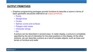
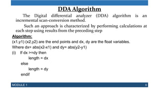
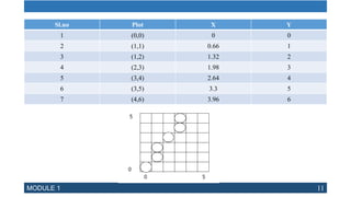
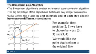
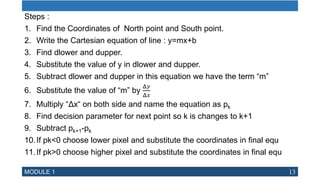
The document discusses computer graphics output primitives and line drawing algorithms. It describes points, lines, polygons and other basic geometric structures used to describe scenes in graphics. It then explains two common line drawing algorithms - the Digital Differential Analyzer (DDA) algorithm and Bresenham's line drawing algorithm. Bresenham's algorithm uses only integer calculations to efficiently rasterize lines and is often used in computer graphics.

1. MODULE 1 1
DEPARTMENT OF COMPUTER SCIENCE AND ENGINEERING
COURSE CODE: 22CS401
COURSE TITLE : COMPUTER GRAPHICS AND MULTIMEDIA

2. OUTPUT PRIMITIVES
Graphics programming packages provide functions to describe a scene in terms of
basic geometric structures referred to as output primitives.
• Points
• Straight lines
• Circles
• Splines curves and surfaces
• Polygon color areas
• Character strings
• Etc.
A picture can be described in several ways. In raster display, a picture is completely
specified by the set of intensities for the pixel positions in the display. At the other
extreme, we can describe a picture as a set of complex objects, such as trees and
terrain or furniture and walls
MODULE 1 2

3. POINTS
The electron beam is turned on to illuminate the phosphor at the selected
location (x, y) where
0 ≤ x ≤ maxx
0 ≤ y ≤ maxy
• setpixel(x, y, intensity) – loads an intensity value into the frame-buffer at
(x, y).
• getpixel(x, y) – retrieves the current frame-buffer intensity setting at
position (x, y).
MODULE 1 3
(0,0)
(maxx,maxy)

4. LINE
A line connects two points. It is a basic element in graphics. To draw a
line, you need two points between which you can draw a line. We refer
the one point of line as X0,Y0 and the second point of line as X1,Y1
LINE ATTRIBUTES
Line type
Solid lines, dashed lines, and dotted lines
Line Width
It is assigned a positive number to indicate the relative width of the line to be
displayed..
Line Color
Color by setting this color value in the framebuffer at pixel locations along
the line path
MODULE 1 4

5. Line Drawing Algorithms
The process of ‘turning on’ the pixels for a line segment is called vector
generation or line generation, and the algorithms for them are known as
vector generation algorithms or line drawing algorithms.
MODULE 1 5
Cartesian equation:
y = mx + c
where
m – slope
c – y-intercept
x1
y1
x2
y2
x
y
x
x
y
y
m






1
2
1
2

6. 6
if |m| = 1
 = 45°
45°
45°
+ve -ve
°
°
°
°
if |m|  1
-45° <  < 45°
if |m|  1
45° <  < 90° or
-90° <  < -45°
Line drawing is accomplished by calculating intermediate positions along the line path between specified end
points.
MODULE 1

7. MODULE 1 7
>

8. DDA Algorithm
The Digital differential analyzer (DDA) algorithm is an
incremental scan-conversion method.
Such an approach is characterized by performing calculations at
each step using results from the preceding step
Algorithm:
(x1,y1) (x2,y2) are the end points and dx, dy are the float variables.
Where dx= abs(x2-x1) and dy= abs(y2-y1)
(i) If dx >=dy then
length = dx
else
length = dy
endif
MODULE 1 8

9. (ii) dx = (x2-x1)/length
dy = (y2-y1)/length
(iii) x = x1 + 0.5
y = y1 + 0.5
(iv) i = 0
(v) While(i<=length)
(vi) x = x + dx
y = y + dy
(v) Plot ((x), (y))
(vii) i = i + 1
Limitations of DDA:
(1) The rounding operation & floating point arithmetic are time consuming
procedures.
(2) Round-off error can cause the calculated pixel position to drift away from the
true line path for long line segment.
MODULE 1 9

10. • Example 1: consider the line from (0,0) to (4,6). Use the simple DDA
algorithm to rasterize this line
Solution:
• x1=0 y1=0 x2=4 y2=6
• Length = 𝑦2− 𝑦1 =6
• Δ𝑥 = (𝑥2 − 𝑥1)/𝑙𝑒𝑛𝑔𝑡ℎ= 4/6
• and Δ𝑦 = (𝑦2 − 𝑦1)/𝑙𝑒𝑛𝑔𝑡ℎ=6/6 = 1
• Initial value for
MODULE 1 10

11. Sl.no Plot X Y
1 (0,0) 0 0
2 (1,1) 0.66 1
3 (1,2) 1.32 2
4 (2,3) 1.98 3
5 (3,4) 2.64 4
6 (3,5) 3.3 5
7 (4,6) 3.96 6
MODULE 1 11

12. The Bresenham Line Algorithm
•The Bresenham algorithm is another incremental scan conversion algorithm
•The big advantage of this algorithm is that it uses only integer calculations
•Move across the x axis in unit intervals and at each step choose
between two different y coordinates
MODULE 1 12
2 3 4 5
2
4
3
5
(xk, yk)
(xk+1, yk)
(xk+1, yk+1)
For example, from
position (2, 3) we have
to choose between (3,
3) and (3, 4)
We would like the
point that is closer to
the original line

13. Steps :
1. Find the Coordinates of North point and South point.
2. Write the Cartesian equation of line : y=mx+b
3. Find dlower and dupper.
4. Substitute the value of y in dlower and dupper.
5. Subtract dlower and dupper in this equation we have the term “m”
6. Substitute the value of “m” by
Δ𝑦
Δ𝑥
7. Multiply “Δx“ on both side and name the equation as pk
8. Find decision parameter for next point so k is changes to k+1
9. Subtract pk+1-pk
10.If pk<0 choose lower pixel and substitute the coordinates in final equ
11.If pk>0 choose higher pixel and substitute the coordinates in final equ
MODULE 1 13

14. Deriving The Bresenham Line Algorithm
At sample position xk+1 the vertical separations from the mathematical line
are labelled dupper and dlower
MODULE 1 14
y
yk
yk+1
xk+1
dlower
dupper
b
x
m
y k 

 )
1
(

15. • So, dupper and dlower are given as follows:
dlower = y – yk= m(xk + 1) + b – yk -----------------------------------1
dupper = yk + 1 – y = yk+ 1– m(xk + 1) – b-------------- 2
Subtract dlower - dupper
dlower-dupper = m(xk + 1) + b – yk- yk-1+ m(xk + 1) + b
• The difference between these two separations is
• dlower – dupper = 2m(xk + 1)–2yk + 2b – 1
MODULE 1 15

16. MODULE 1 16
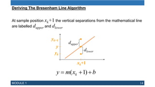
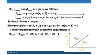
dlower – dupper = 2m(xk + 1)–2yk + 2b – 1
Let’s substitute m with ∆y/∆x where ∆x and ∆y are the differences
between the end-points:
dlower – dupper = [2(∆y/∆x)(xk + 1) ]– 2yk + 2b – 1
Multiplying both side by (∆x)
= [ 2∆y xk+ 2∆y – 2∆x yk + 2∆x b – ∆x]
= [ 2∆y xk – 2∆x yk + 2∆x b – ∆x + 2∆y]
= [ 2∆y xk – 2∆x yk + c]
Where c = 2∆x b – ∆x + 2∆y
∆x (dlower – dupper) = 2∆y xk – 2∆x yk + c

17. ∆x (dlower – dupper) = 2∆y xk – 2∆x yk + c
• This equation is used as a simple decision about which pixel is closer to
the mathematical line.
• So, a decision parameter pk for the kth step along a line is given by:
pk = ∆x (dlower – dupper) = 2∆y xk – 2∆x yk + c
• The sign of the decision parameter pk is the same the sign of dlower–dupper,
• if the pixel at yk is closer to the line path than the pixel at yk+1 (that is
dlower<dupper), then decision parameter pk is negative. In this case we plot
the lower pixel, otherwise we plot the upper pixel.
MODULE 1 17

18. Coordinate changes along the line occur in unit steps in either the x or y directions.
Therefore, we can obtain the values of successive decision parameters using
incremental integer calculations.
At step k+1 the decision parameter is given as:
pk+1 = 2∆y xk+1 – 2∆x yk+1 + c
Subtracting pk from this we get:
pk+1 – pk = 2∆y( xk+1– xk ) – 2∆x( yk+1 – yk )
If pk < 0, the next point to plot is (xk+1, yk) and
pk+1 = pk + 2∆y
Otherwise, the next point to plot is (xk+1, yk+1) and
pk+1 = pk + 2∆y – 2∆x
MODULE 1 18

19. Bresenham ’s Line Drawing Algorithm
The recursive calculation of decision parameters is performed at
each integer x position, starting at the left coordinate endpoint of
the line.
The first decision parameter p0 is evaluated at the starting pixel
position (x0, y0) and with m evaluated as (∆y/∆x):
P0 = 2∆y – ∆x
The following steps summarize Bresenham’s Line Drawing
Algorithm for a line with positive slope less than 1 (|m|<1)
MODULE 1 19

20. Bresenham ’s Line Drawing Algorithm
1.Input the two line end-points, storing the left end-point in (x0,y0)
2.Plot the point (x0, y0)
3.Calculate the constants Δx, Δy, 2Δy, and (2Δy - 2Δx) and get the first value for
the decision parameter as:
P0 = 2∆y – ∆x
4.At each xk along the line, starting at k=0, perform the following test:
If pk < 0, the next point to plot is (xk+1, yk) and
pk+1 = pk + 2∆y
Otherwise, the next point to plot is (xk+1, yk+1) and
pk+1 = pk + 2∆y – 2∆x
5.Repeat step 4 (Δx ) times
MODULE 1 20

21. Bresenham ’s Line Drawing Algorithm
Bresenham’s Line Drawing Example
To illustrate the algorithm, we digitize the line with endpoints(20,10) and (30,
18). This line has a slope of 0.8, with
Δx =10, Δy = 8
The initial decision parameter has the value P0 = 2∆y – ∆x = 6
And the increments for calculation successive decision parameters are:
2Δy = 16,
2Δy – 2Δx= – 4
We plot the initial point (20, 10) , and determine successive pixel positions along
the line path from the decision parameters as:
MODULE 1 21

22. MODULE 1 22
k pk (xk+1, yk+1)
0 6 (21, 11)
1 2 (22, 12)
2 -2 (23, 12)
3 14 (24, 13)
4 10 (25, 14)
5 6 (26, 15)
6 2 (27, 16)
7 -2 (28, 16)
8 14 (29, 17)
9 10 (30, 18)
• If pk < 0, (xk+1, yk)
pk+1 = pk + 2∆y
If pk >0 , (xk+1, yk+1)
pk+1 = pk + 2∆y – 2∆x
2Δy = 16,
2Δy – 2Δx= – 4
Bresenham ’ Line Drawing Algorithm
Bresenham’s Line Drawing Example