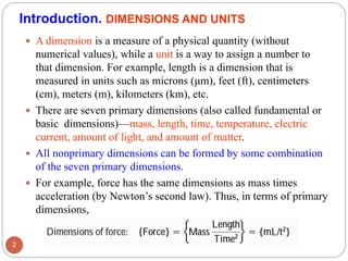
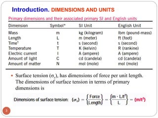
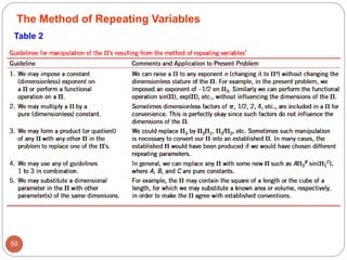
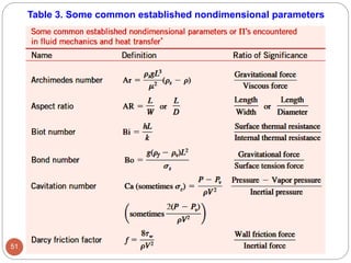
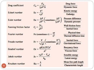
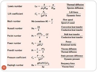
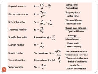
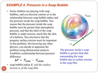
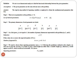
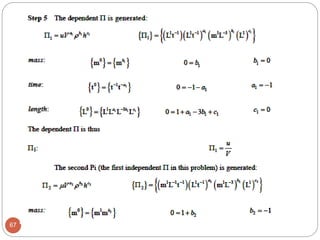
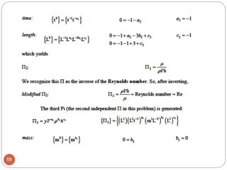
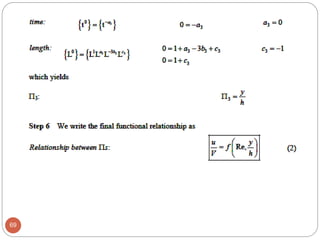
SlideShare a Scribd company logo
1
Dimensional Analysis And Similitude
Chapter 5
Fluid Mechanics
(MEng 2113)
Mechanical Engineering
Department
Prepared by: Addisu Dagne May, 2016
Introduction. DIMENSIONS AND UNITS
 A dimension is a measure of a physical quantity (without
numerical values), while a unit is a way to assign a number to
that dimension. For example, length is a dimension that is
measured in units such as microns (μm), feet (ft), centimeters
(cm), meters (m), kilometers (km), etc.
 There are seven primary dimensions (also called fundamental or
basic dimensions)—mass, length, time, temperature, electric
current, amount of light, and amount of matter.
 All nonprimary dimensions can be formed by some combination
of the seven primary dimensions.
 For example, force has the same dimensions as mass times
acceleration (by Newton’s second law). Thus, in terms of primary
dimensions,
2
 Surface tension (σs), has dimensions of force per unit length.
The dimensions of surface tension in terms of primary
dimensions is
3
Introduction. DIMENSIONS AND UNITS
DIMENSIONAL HOMOGENEITY
 Law of dimensional homogeneity: Every additive term in an
equation must have the same dimensions.
 Consider, for example, the change in total energy of a simple
compressible closed system from one state and/or time (1) to
another (2), as shown in the figure
4
 The change in total energy of the
system (∆E) is given by
 where E has three components:
internal energy (U), kinetic energy
(KE), and potential energy (PE).
 These components can be written in terms of the system mass (m);
measurable quantities and thermodynamic properties at each of the
two states, such as speed (V), elevation (z), and specific internal
energy (u); and the known gravitational acceleration constant (g),
 It is straightforward to verify that the left side of the change in
Energy equation and all three additive terms on the right side have
the same dimensions—energy.
5
DIMENSIONAL HOMOGENEITY
 In addition to dimensional homogeneity, calculations are valid
only when the units are also homogeneous in each additive term.
 For example, units of energy in the above terms may be J, N·m ,
or kg·m2/s2, all of which are equivalent.
 Suppose, however, that kJ were used in place of J for one of the
terms. This term would be off by a factor of 1000 compared to
the other terms.
 It is wise to write out all units when performing mathematical
calculations in order to avoid such errors.
6
DIMENSIONAL HOMOGENEITY
Example 1. Dimensional Homogeneity of the Bernoulli
Equation
 Probably the most well-known equation in fluid mechanics is
the Bernoulli equation . One standard form of the Bernoulli
equation for incompressible irrotational fluid flow is
 (a) Verify that each additive term in the Bernoulli equation
has the same dimensions. (b) What are the dimensions of the
constant C?
7
8
Example 2 . Dimensional Homogeneity
 In Chap. 4 we discussed the differential equation for conservation
of mass, the continuity equation. In cylindrical coordinates, and for
steady flow,
 Write the primary dimensions of each additive term in the equation,
and verify that the equation is dimensionally homogeneous.
9
 Solution. We are to determine the primary dimensions of each
additive term, and we are to verify that the equation is dimensionally
homogeneous.
 Analysis .The primary dimensions of the velocity components are
length/time. The primary dimensions of coordinates r and z are
length, and the primary dimensions of coordinate θ are unity (it is a
dimensionless angle). Thus each term in the equation can be written
in terms of primary dimensions,
10
Example 2 . Dimensional Homogeneity
 Indeed, all three additive terms have the same dimensions,
namely {t-1}.
Nondimensionalization of Equations
 The law of dimensional
homogeneity guarantees that
every additive term in an
equation has the same
dimensions.
 It follows that if we divide
each term in the equation by a
collection of variables and
constants whose product has
those same dimensions, the
equation is rendered
nondimensional.
11
 If, in addition, the nondimensional terms in the equation are of
order unity, the equation is called normalized.
 Each term in a nondimensional equation is dimensionless.
A nondimensionalized form of the
Bernoulli equation is formed by
dividing each additive term by a
pressure (here we use ). Each
resulting term is dimensionless
(dimensions of {1}).
 In the process of nondimensionalizing an equation of motion,
nondimensional parameters often appear—most of which are
named after a notable scientist or engineer (e.g., the Reynolds
number and the Froude number).
 This process is sometimes called inspectional analysis.
 As a simple example, consider the equation of motion
describing the elevation z of an object falling by gravity
through a vacuum (no air drag).
 The initial location of the object is z0 and its initial velocity is
w0 in the z-direction. From high school physics,
……………… (1)
 Dimensional variables are defined as dimensional quantities
that change or vary in the problem.
12
Nondimensionalization of Equations
 For the simple differential equation given in Eq. 1, there are
two dimensional variables: z (dimension of length) and t
(dimension of time).
 Nondimensional (or dimensionless) variables are defined as
quantities that change or vary in the problem, but have no
dimensions; an example is angle of rotation, measured in
degrees or radians which are dimensionless units. Gravitational
constant g, while dimensional, remains constant and is called a
dimensional constant.
 Other dimensional constants are relevant to this particular
problem are initial location z0 and initial vertical speed w0.
 While dimensional constants may change from problem to
problem, they are fixed for a particular problem and are thus
distinguished from dimensional variables.
13
Nondimensionalization of Equations
 We use the term parameters for the combined set of
dimensional variables, nondimensional variables, and
dimensional constants in the problem.
 Equation 1 is easily solved by integrating twice and
applying the initial conditions. The result is an expression
for elevation z at any time t:
……………(2)
 The constant ½ and the exponent 2 in Eq. 2 are
dimensionless results of the integration. Such constants are
called pure constants. Other common examples of pure
constants are Π and e.
14
Nondimensionalization of Equations
 To nondimensionalize Eq.
1, we need to select
scaling parameters,
based on the primary
dimensions contained in
the original equation.
 In fluid flow problems
there are typically at least
three scaling parameters,
e.g., L, V, and ,
since there are at least
three primary dimensions
in the general problem
(e.g., mass, length, and
time).15
Nondimensionalization of Equations
In a typical fluid flow problem, the
scaling parameters usually include a
characteristic length L, a characteristic
velocity V, and a reference pressure
difference . Other parameters
and fluid properties such as density,
viscosity, and gravitational acceleration
enter the problem as well.
 In the case of the falling object being discussed here, there are
only two primary dimensions, length and time, and thus we are
limited to selecting only two scaling parameters.
 We have some options in the selection of the scaling parameters
since we have three available dimensional constants g, z0, and
w0. We choose z0 and w0. we can also do the analysis using g and
z0 and/or with g and w0
 With these two chosen scaling parameters we nondimensionalize
the dimensional variables z and t.
 The first step is to list the primary dimensions of all dimensional
variables and dimensional constants in the problem,
Primary dimensions of all parameters:
16
Nondimensionalization of Equations
 The second step is to use our two scaling parameters to
nondimensionalize z and t (by inspection) into nondimensional
variables z* and t*,
Nondimensionalized variables:
………………(3)
 Substitution of Eq. 3 into Eq. 1 gives
 …...(4)
 which is the desired nondimensional equation. The grouping of
dimensional constants in Eq. 4 is the square of a well-known
nondimensional parameter or dimensionless group called the
Froude number,17
Nondimensionalization of Equations
 Froude number: ………... (5)
 Substitution of Eq. 5 into Eq. 4 yields
 Nondimensionalized equation of motion: …..(6)
 In dimensionless form, only one parameter remains, namely the
Froude number.
 Equation 6 is easily solved by integrating twice and applying the
initial conditions. The result is an expression for dimensionless
elevation z* as a function of dimensionless time t*:
 Nondimensional result:
 …………(7)
18
Nondimensionalization of Equations
 There are two key advantages of nondimensionalization
 First, it increases our insight about the relationships between
key parameters. Equation 5 reveals, for example, that doubling
w0 has the same effect as decreasing z0 by a factor of 4.
 Second, it reduces the number of parameters in the problem.
For example, the original problem contains one dependent
variable, z; one independent variable, t; and three additional
dimensional constants, g, w0, and z0. The nondimensionalized
problem contains one dependent parameter, z*; one
independent parameter, t*; and only one additional parameter,
namely the dimensionless Froude number, Fr. The number of
additional parameters has been reduced from three to one!
19
Nondimensionalization of Equations
Dimensional Analysis and Similarity
 Nondimensionalization of an equation by inspection is useful
only when we know the equation to begin with.
 However, in many cases in real-life engineering, the equations
are either not known or too difficult to solve; often times
experimentation is the only method of obtaining reliable
information.
 In most experiments, to save time and money, tests are
performed on a geometrically scaled model, rather than on the
full-scale prototype. In such cases, care must be taken to
properly scale the results. We introduce here a powerful
technique called dimensional analysis.
20
 The three primary purposes of dimensional analysis are
✓To generate nondimensional parameters that help in the
design of experiments (physical and/or numerical) and in
the reporting of experimental results
✓To obtain scaling laws so that prototype performance can
be predicted from model performance
✓To (sometimes) predict trends in the relationship between
parameters
 There are three necessary conditions for complete similarity
between a model and a prototype.
 The first condition is geometric similarity—the model must
be the same shape as the prototype, but may be scaled by
some constant scale factor.
21
Dimensional Analysis and Similarity
 The second condition is
kinematic similarity, which
means that the velocity at
any point in the model flow
must be proportional (by a
constant scale factor) to the
velocity at the
corresponding point in the
prototype flow.
 Specifically, for kinematic
similarity the velocity at
corresponding points must
scale in magnitude and must
point in the same relative
direction.22
Dimensional Analysis and Similarity
Fig. Kinematic similarity
23
 Kinematic similarity is achieved when, at all locations, the speed in
the model flow is proportional to that at corresponding locations in
the prototype flow, and points in the same direction.
 Geometric similarity is a prerequisite for kinematic similarity
 Just as the geometric scale factor can be less than, equal to, or
greater than one, so can the velocity scale factor.
 In Fig. above, for example, the geometric scale factor is less than
one (model smaller than prototype), but the velocity scale is greater
than one (velocities around the model are greater than those around
the prototype).
 The third and most restrictive similarity condition is that of
dynamic similarity. Dynamic similarity is achieved when all
forces in the model flow scale by a constant factor to corresponding
forces in the prototype flow (force-scale equivalence).
Dimensional Analysis and Similarity
 As with geometric and kinematic similarity, the scale factor for
forces can be less than, equal to, or greater than one.
 In Fig. shown in slide 20 above for example, the force-scale
factor is less than one since the force on the model building is
less than that on the prototype.
 Kinematic similarity is a necessary but insufficient condition
for dynamic similarity.
 It is thus possible for a model flow and a prototype flow to
achieve both geometric and kinematic similarity, yet not
dynamic similarity. All three similarity conditions must exist for
complete similarity to be ensured.
 In a general flow field, complete similarity between a model
and prototype is achieved only when there is geometric,
kinematic, and dynamic similarity.
24
Dimensional Analysis and Similarity
 We let uppercase Greek letter Pi (Π) denote a nondimensional
parameter. We have already discussed one Π, namely the
Froude number, Fr.
 In a general dimensional analysis problem, there is one Π that
we call the dependent Π, giving it the notation Π1. The
parameter Π1 is in general a function of several other Π’s,
which we call independent Π’s. The functional relationship is
 Functional relationship between Π’s:
 where k is the total number of Π’s.
 Consider an experiment in which a scale model is tested to
simulate a prototype flow.
25
Dimensional Analysis and Similarity
 To ensure complete similarity between the model and the
prototype, each independent P of the model (subscript m) must
be identical to the corresponding independent Π of the prototype
(subscript p),
i.e., Π2, m = Π2, p , Π3, m = Π3, p, . . . .., Πk, m = Πk, p.
 To ensure complete similarity, the model and prototype must be
geometrically similar, and all independent Π groups must match
between model and prototype.
 Under these conditions the dependent Π of the model (Π1, m) is
guaranteed to also equal the dependent Π of the prototype (Π1, p).
 Mathematically, we write a conditional statement for achieving
similarity,
26
Dimensional Analysis and Similarity
 Consider, for example, the
design of a new sports car, the
aerodynamics of which is to
be tested in a wind tunnel. To
save money, it is desirable to
test a small, geometrically
scaled model of the car rather
than a full-scale prototype of
the car.
 In the case of aerodynamic
drag on an automobile, it
turns out that if the flow is
approximated as
incompressible, there are only
two Π’s in the problem,27
Dimensional Analysis and Similarity
 Where
 The procedure used to generate these Π’s will be discussed
later in this chapter.
 In the above equation FD is the magnitude of the aerodynamic
drag on the car, ρ is the air density, V is the car’s speed (or the
speed of the air in the wind tunnel), L is the length of the car,
and μ is the viscosity of the air. Π1 is a nonstandard form of the
drag coefficient, and Π2 is the Reynolds number, Re.
 The Reynolds number is the most well known and useful
dimensionless parameter in all of fluid mechanics
28
Dimensional Analysis and Similarity
 In the problem at hand there is only one independent Π, and
the above Eq. ensures that if the independent Π’s match (the
Reynolds numbers match: Π2, m = Π2, p ), then the dependent
Π’s also match (Π1, m = Π1, p).
 This enables engineers to measure the aerodynamic drag on
the model car and then use this value to predict the
aerodynamic drag on the prototype car.
29
Dimensional Analysis and Similarity
Example 3: Similarity between Model and Prototype Cars
 The aerodynamic drag of a new sports car is to be predicted at a
speed of 50.0 mi/h at an air temperature of 25°C. Automotive
engineers build a one fifth scale model of the car to test in a wind
tunnel. It is winter and the wind tunnel is located in an unheated
building; the temperature of the wind tunnel air is only about
5°C. Determine how fast the engineers should run the wind
tunnel in order to achieve similarity between the model and the
prototype.
Solution:
 We are to utilize the concept of similarity to determine the speed
of the wind tunnel.
Assumptions:
 The model is geometrically similar to the prototype
 The wind tunnel walls are far enough away so as to not interfere
with the aerodynamic drag on the model car.30
 The wind tunnel has a moving belt to simulate the ground under
the car. (The moving belt is necessary in order to achieve
kinematic similarity everywhere in the flow, in particular
underneath the car.)
31
Example 3: Similarity between Model and Prototype Cars
A drag balance is a device
used in a wind tunnel to
measure the aerodynamic
drag of a body. When
testing automobile models,
a moving belt is often
added to the floor of the
wind tunnel to simulate the
moving ground
(from the car’s frame of
reference).
 Properties: For air at atmospheric pressure and at T = 25°C, ρ =
1.184 kg/m3 and μ = 1.849 x 10⁻⁵ kg/m·s. Similarly, at T = 5°C,
ρ = 1.269 kg/m3 and μ = 1.754 x 10⁻⁵ kg/m·s.
 Analysis: Since there is only one independent Π in this problem,
the similarity equation holds if Π2, m = Π2, p, where Π2 is the
Reynolds number. Thus, we write
 Thus
32
Example 3: Similarity between Model and Prototype Cars
 The power of using dimensional analysis and similarity to
supplement experimental analysis is further illustrated by the fact
that the actual values of the dimensional parameters (density,
velocity, etc.) are irrelevant. As long as the corresponding
independent Π’s are set equal to each other, similarity is achieved
even if different fluids are used.
 This explains why automobile or aircraft performance can be
simulated in a water tunnel, and the performance of a submarine can
be simulated in a wind tunnel.
 Suppose, for example, that the engineers in Example above use a
water tunnel instead of a wind tunnel to test their one-fifth scale
model. Using the properties of water at room temperature (20°C is
assumed), the water tunnel speed required to achieve similarity is
easily calculated as
33
Example 3: Similarity between Model and Prototype Cars
 As can be seen, one advantage of a water tunnel is that the
required water tunnel speed is much lower than that required
for a wind tunnel using the same size model
34
Example 3: Similarity between Model and Prototype Cars
The Method of Repeating Variables and the
Buckingham Pi Theorem
 In this section we will learn how to generate the nondimensional
parameters, i.e., the Π’s.
 There are several methods that have been developed for this
purpose, but the most popular (and simplest) method is the method
of repeating variables, popularized by Edgar Buckingham (1867–
1940).
 We can think of this method as a step-by-step procedure or
“recipe” for obtaining nondimensional parameters. There are six
steps in this method as described below in detail
35
36
The Method of Repeating Variables and the
Buckingham Pi Theorem
37
The Method of Repeating Variables and the
Buckingham Pi Theorem
 Fig. A concise
summary of the six
steps that comprise
the method of
repeating variables
38
The Method of Repeating Variables and the
Buckingham Pi Theorem
 As a simple first example, consider a ball falling in a vacuum. Let
us pretend that we do not know that Eq. 1 is appropriate for this
problem, nor do we know much physics concerning falling objects.
 In fact, suppose that all we know is that the instantaneous
elevation z of the ball must be a function of time t, initial vertical
speed w0, initial elevation z0, and gravitational constant g.
 The beauty of dimensional analysis is that the only other thing we
need to know is the primary dimensions of each of these
quantities.
 As we go through each step of the method of repeating variables,
we explain some of the subtleties of the technique in more detail
using the falling ball as an example.
39
The Method of Repeating Variables and the
Buckingham Pi Theorem
The Method of Repeating Variables
Step 1
 There are five parameters
(dimensional variables,
nondimensional
variables, and
dimensional constants) in
this problem; n = 5. They
are listed in functional
form, with the dependent
variable listed as a
function of the
independent variables
and constants:
 List of relevant
parameters:
40
Fig. Setup for dimensional analysis of a ball falling
in a vacuum. Elevation z is a function of time t,
initial vertical speed w0, initial elevation z0, and
gravitational constant g.
41
The Method of Repeating Variables
Step 4
 We need to choose two repeating parameters since j = 2. Since
this is often the hardest (or at least the most mysterious) part of
the method of repeating variables, several guidelines about
choosing repeating parameters are listed in Table 1.
 Following the guidelines of Table 1 on the next page, the wisest
choice of two repeating parameters is w0 and z0.
Repeating parameters: w0 and z0
Step 5
 Now we combine these repeating parameters into products with
each of the remaining parameters, one at a time, to create the Π’s.
The first Π is always the dependent Π and is formed with the
dependent variable z.
Dependent Π : ……………….(1)
 where a1 and b1 are constant exponents that need to be determined.42
The Method of Repeating Variables
 We apply the primary dimensions of step 2 into Eq. 1 and force
the Π to be dimensionless by setting the exponent of each
primary dimension to zero:
 Dimensions of Π1:
 Since primary dimensions are by definition independent of each
other, we equate the exponents of each primary dimension
independently to solve for exponents a1 and b1
 Thus
43
The Method of Repeating Variables
 In similar fashion we create the first independent Π (Π2) by
combining the repeating parameters with independent variable t.
44
The Method of Repeating Variables
 Finally we create the second independent Π (Π3) by combining
the repeating parameters with g and forcing the P to be
dimensionless
45
The Method of Repeating Variables
 We can see that Π1 and Π2 are the same as the nondimensionalized
variables z* and t* defined by Eq. 3 (See slide number 15)—no
manipulation is necessary for these.
 However, we recognize that the third P must be raised to the power
of -1/2 to be of the same form as an established dimensionless
parameter, namely the Froude number of
 Such manipulation is often necessary to put the Π’s into proper
established form (“socially acceptable form” since it is a named,
established nondimensional parameter that is commonly used in
the literature.
46
The Method of Repeating Variables
Step 6
 We should double-check that the Π’s are indeed dimensionless
 We are finally ready to write the functional relationship between
the nondimensional parameters
Relationship between Π’s:
 The method of repeating variables properly predicts the functional
relationship between dimensionless groups.
 However, the method of repeating variables cannot predict the
exact mathematical form of the equation. This is a fundamental
limitation of dimensional analysis and the method of repeating
variables.
47
The Method of Repeating Variables
48
The Method of Repeating Variables
Table 1
49
The Method of Repeating Variables
50
The Method of Repeating Variables
Table 2
51
Table 3. Some common established nondimensional parameters
52
53
54
EXAMPLE 4. Pressure in a Soap Bubble
 Some children are playing with soap
bubbles, and you become curious as to the
relationship between soap bubble radius and
the pressure inside the soap bubble. You
reason that the pressure inside the soap
bubble must be greater than atmospheric
pressure, and that the shell of the soap
bubble is under tension, much like the skin
of a balloon. You also know that the
property surface tension must be important
in this problem. Not knowing any other
physics, you decide to approach the
problem using dimensional analysis.
Establish a relationship between pressure
difference
 soap bubble radius R, and the surface
tension σs of the soap film.55
The pressure inside a soap
bubble is greater than that
surrounding the soap
bubble due to surface tension
in the soap film.
 SOLUTION. The pressure difference between the inside of a soap
bubble and the outside air is to be analyzed by the method of
repeating variables.
 Assumptions 1. The soap bubble is neutrally buoyant in the air, and
gravity is not relevant. 2 No other variables or constants are
important in this problem.
 Analysis The step-by-step method of repeating variables is
employed.
56
EXAMPLE 4. Pressure in a Soap Bubble
 Step 2 The primary dimensions of each parameter are listed.
 Step 3 As a first guess, j is set equal to 3, the number of primary
dimensions represented in the problem (m, L, and t).
Reduction (first guess): j = 3
 If this value of j is correct, the expected number of Π’s is
k = n - j = 3 - 3 = 0.
But how can we have zero P’s? Something is obviously not right
 At times like this, we need to first go back and make sure that we are
not neglecting some important variable or constant in the problem.
 Since we are confident that the pressure difference should depend only
on soap bubble radius and surface tension, we reduce the value of j by
one,
57
EXAMPLE 4. Pressure in a Soap Bubble
Reduction (second guess): j = 2
 If this value of j is correct, k = n - j = 3 - 2 = 1. Thus we expect one
Π, which is more physically realistic than zero Π’s.
 Step 4 We need to choose two repeating parameters since j = 2.
Following the guidelines of Table 1, our only choices are R and σs,
since ∆P is the dependent variable.
 Step 5 We combine these repeating parameters into a product with
the dependent variable ∆P to create the dependent Π,
Dependent Π: ………(1)
 We apply the primary dimensions of step 2 into Eq. 1 and force the
Π to be dimensionless.
58
EXAMPLE 4. Pressure in a Soap Bubble
 From Table 3, the established nondimensional parameter most
similar to Eq. 2 is the Weber number, defined as a pressure
(ρV2) times a length divided by surface tension. There is no need
to further manipulate this Π.
59
EXAMPLE 4. Pressure in a Soap Bubble
 Step 6 We write the final functional relationship. In the case at
hand, there is only one Π, which is a function of nothing. This is
possible only if the Π is constant.
 Relationship between Π’s:
 This is an example of how we can sometimes predict trends with
dimensional analysis, even without knowing much of the physics
of the problem. For example, we know from our result that if the
radius of the soap bubble doubles, the pressure difference
decreases by a factor of 2. Similarly, if the value of surface
tension doubles, ∆P increases by a factor of 2.
 Dimensional analysis cannot predict the value of the constant in
Eq. 3; further analysis (or one experiment) reveals that the
constant is equal to 4 (Chap. 1).
60
EXAMPLE 4. Pressure in a Soap Bubble
Example 5
 When small aerosol particles or microorganisms move through
air or water, the Reynolds number is very small (Re << 1). Such
flows are called creeping flows. The aerodynamic drag on an
object in creeping flow is a function only of its speed V, some
characteristic length scale L of the object, and fluid viscosity μ.
Use dimensional analysis to generate a relationship for FD as a
function of the independent variables.
61
62
63
64
Example 6
 Consider fully developed Couette flow—flow between two infinite
parallel plates separated by distance h, with the top plate moving
and the bottom plate stationary as illustrated in the Fig. shown. The
flow is steady, incompressible, and two-dimensional in the xy-plane.
Use the method of repeating variables to generate a dimensionless
relationship for the x component of fluid velocity u as a function of
fluid viscosity μ, top plate speed V, distance h, fluid density ρ, and
distance y.
65
66
67
68
69
End of Chapter 5
Next Lecture
Chapter 6: Boundary Layer Concept
70

More Related Content

What's hot

friction loss along a pipe
friction loss along a pipefriction loss along a pipe
friction loss along a pipe
Saif al-din ali
 
Boundary layer theory
Boundary layer theoryBoundary layer theory
Boundary layer theory
Manthan Chavda
 
navier stokes equation
navier stokes equationnavier stokes equation
navier stokes equation
Karan Patel
 
Fluid kinematics
Fluid kinematicsFluid kinematics
Fluid kinematics
Mohsin Siddique
 
Fluid Mechanics Chapter 2 Part II. Fluids in rigid-body motion
Fluid Mechanics Chapter 2 Part II. Fluids in rigid-body motionFluid Mechanics Chapter 2 Part II. Fluids in rigid-body motion
Fluid Mechanics Chapter 2 Part II. Fluids in rigid-body motion
Addisu Dagne Zegeye
 
Fluid Flow Rate & Bernoulli’s Theorem Demonstration
Fluid Flow Rate & Bernoulli’s Theorem DemonstrationFluid Flow Rate & Bernoulli’s Theorem Demonstration
Fluid Flow Rate & Bernoulli’s Theorem Demonstration
Raboon Redar
 
Hydraulic similitude and model analysis
Hydraulic similitude and model analysisHydraulic similitude and model analysis
Hydraulic similitude and model analysis
Mohsin Siddique
 
Couette flow
Couette flowCouette flow
Couette flow
Kumar Virendra
 
Terbulent Flow in fluid mechanics
Terbulent Flow in fluid mechanicsTerbulent Flow in fluid mechanics
Terbulent Flow in fluid mechanics
Pavan Narkhede
 
Introduction to fluid mechanics
Introduction to fluid mechanicsIntroduction to fluid mechanics
Introduction to fluid mechanics
Mohsin Siddique
 
PRESSURE & HEAD (PART-1)
PRESSURE & HEAD (PART-1)PRESSURE & HEAD (PART-1)
PRESSURE & HEAD (PART-1)
KHORASIYA DEVANSU
 
Chapter 1. introduction to fluid mechanics
Chapter 1. introduction to fluid mechanicsChapter 1. introduction to fluid mechanics
Chapter 1. introduction to fluid mechanics
kidanemariam tesera
 
Fluid discharge
Fluid dischargeFluid discharge
Fluid discharge
Keith Vaugh
 
Buoyancy and floatation
Buoyancy and floatationBuoyancy and floatation
Buoyancy and floatation
Mohsin Siddique
 
Fluid dynamic
Fluid dynamicFluid dynamic
Fluid dynamic
Mohsin Siddique
 
Boundary layer equation
Boundary layer equationBoundary layer equation
Boundary layer equationJustin Myint
 
Fluid Mechanics Chapter 2. Fluid Statics
Fluid Mechanics Chapter 2. Fluid StaticsFluid Mechanics Chapter 2. Fluid Statics
Fluid Mechanics Chapter 2. Fluid Statics
Addisu Dagne Zegeye
 
Chapter four fluid mechanics
Chapter four fluid mechanicsChapter four fluid mechanics
Chapter four fluid mechanics
abrish shewa
 
Fluid mechanics(2130602)
Fluid mechanics(2130602)Fluid mechanics(2130602)
Fluid mechanics(2130602)
Sujith Velloor Sudarsanakumar Nair
 
Fluid mech. lec midterm coverage
Fluid mech. lec   midterm coverageFluid mech. lec   midterm coverage
Fluid mech. lec midterm coverage
Shobbbe
 

What's hot (20)

friction loss along a pipe
friction loss along a pipefriction loss along a pipe
friction loss along a pipe
 
Boundary layer theory
Boundary layer theoryBoundary layer theory
Boundary layer theory
 
navier stokes equation
navier stokes equationnavier stokes equation
navier stokes equation
 
Fluid kinematics
Fluid kinematicsFluid kinematics
Fluid kinematics
 
Fluid Mechanics Chapter 2 Part II. Fluids in rigid-body motion
Fluid Mechanics Chapter 2 Part II. Fluids in rigid-body motionFluid Mechanics Chapter 2 Part II. Fluids in rigid-body motion
Fluid Mechanics Chapter 2 Part II. Fluids in rigid-body motion
 
Fluid Flow Rate & Bernoulli’s Theorem Demonstration
Fluid Flow Rate & Bernoulli’s Theorem DemonstrationFluid Flow Rate & Bernoulli’s Theorem Demonstration
Fluid Flow Rate & Bernoulli’s Theorem Demonstration
 
Hydraulic similitude and model analysis
Hydraulic similitude and model analysisHydraulic similitude and model analysis
Hydraulic similitude and model analysis
 
Couette flow
Couette flowCouette flow
Couette flow
 
Terbulent Flow in fluid mechanics
Terbulent Flow in fluid mechanicsTerbulent Flow in fluid mechanics
Terbulent Flow in fluid mechanics
 
Introduction to fluid mechanics
Introduction to fluid mechanicsIntroduction to fluid mechanics
Introduction to fluid mechanics
 
PRESSURE & HEAD (PART-1)
PRESSURE & HEAD (PART-1)PRESSURE & HEAD (PART-1)
PRESSURE & HEAD (PART-1)
 
Chapter 1. introduction to fluid mechanics
Chapter 1. introduction to fluid mechanicsChapter 1. introduction to fluid mechanics
Chapter 1. introduction to fluid mechanics
 
Fluid discharge
Fluid dischargeFluid discharge
Fluid discharge
 
Buoyancy and floatation
Buoyancy and floatationBuoyancy and floatation
Buoyancy and floatation
 
Fluid dynamic
Fluid dynamicFluid dynamic
Fluid dynamic
 
Boundary layer equation
Boundary layer equationBoundary layer equation
Boundary layer equation
 
Fluid Mechanics Chapter 2. Fluid Statics
Fluid Mechanics Chapter 2. Fluid StaticsFluid Mechanics Chapter 2. Fluid Statics
Fluid Mechanics Chapter 2. Fluid Statics
 
Chapter four fluid mechanics
Chapter four fluid mechanicsChapter four fluid mechanics
Chapter four fluid mechanics
 
Fluid mechanics(2130602)
Fluid mechanics(2130602)Fluid mechanics(2130602)
Fluid mechanics(2130602)
 
Fluid mech. lec midterm coverage
Fluid mech. lec   midterm coverageFluid mech. lec   midterm coverage
Fluid mech. lec midterm coverage
 

Similar to Fluid Mechanics Chapter 5. Dimensional Analysis and Similitude

dimensional_analysis.pptx
dimensional_analysis.pptxdimensional_analysis.pptx
dimensional_analysis.pptx
DinaSaad22
 
Fluid Mechanics
Fluid MechanicsFluid Mechanics
Fluid Mechanics
Umang Parmar
 
dimensioanalysis-180614115528 (1).pdf
dimensioanalysis-180614115528 (1).pdfdimensioanalysis-180614115528 (1).pdf
dimensioanalysis-180614115528 (1).pdf
saptarshichatterjee33
 
Dimensional analysis
Dimensional analysisDimensional analysis
Dimensional analysis
Ronak Parmar
 
1,2. Dimensional Analysis and fluid .pptx
1,2. Dimensional Analysis and fluid .pptx1,2. Dimensional Analysis and fluid .pptx
1,2. Dimensional Analysis and fluid .pptx
MuhammadHabib533231
 
JEE Main 11&12 Sample ebook
JEE Main 11&12 Sample ebookJEE Main 11&12 Sample ebook
JEE Main 11&12 Sample ebook
Miso Study
 
JEE Main Advanced 11 Sample ebook
JEE Main Advanced 11 Sample ebookJEE Main Advanced 11 Sample ebook
JEE Main Advanced 11 Sample ebook
Miso Study
 
JEE Main Advanced 11 & 12th Sample ebook
JEE Main Advanced 11 & 12th Sample ebookJEE Main Advanced 11 & 12th Sample ebook
JEE Main Advanced 11 & 12th Sample ebook
Miso Study
 
Dimensional analysis - Part 1
Dimensional analysis - Part 1 Dimensional analysis - Part 1
Dimensional analysis - Part 1
Ramesh B R
 
Atp (Advancede transport phenomena)
Atp (Advancede transport phenomena)Atp (Advancede transport phenomena)
Atp (Advancede transport phenomena)
Wolkite University
 
Numerical simulation on laminar free convection flow and heat transfer over a...
Numerical simulation on laminar free convection flow and heat transfer over a...Numerical simulation on laminar free convection flow and heat transfer over a...
Numerical simulation on laminar free convection flow and heat transfer over a...
eSAT Journals
 
Mechanics
MechanicsMechanics
Mechanics
shahzadebaujiti
 
Units and dimension.pptx
Units and dimension.pptxUnits and dimension.pptx
Units and dimension.pptx
Shashwatsingh500380
 
UNIT - III.ppt
UNIT - III.pptUNIT - III.ppt
UNIT - III.ppt
AJIN49
 
Second application of dimensional analysis
Second application of dimensional analysisSecond application of dimensional analysis
Second application of dimensional analysis
Jaypee Institute of Information Technology
 
Admissions in India 2015
Admissions in India 2015Admissions in India 2015
Admissions in India 2015
Edhole.com
 
Units , Measurement and Dimensional Analysis
Units , Measurement and Dimensional AnalysisUnits , Measurement and Dimensional Analysis
Units , Measurement and Dimensional Analysis
Oleepari
 
Dimensions and Dimensional Analysis
Dimensions and Dimensional AnalysisDimensions and Dimensional Analysis
Dimensions and Dimensional Analysis
Tanzania Atomic Energy Commission
 

Similar to Fluid Mechanics Chapter 5. Dimensional Analysis and Similitude (20)

dimensional_analysis.pptx
dimensional_analysis.pptxdimensional_analysis.pptx
dimensional_analysis.pptx
 
Fluid Mechanics
Fluid MechanicsFluid Mechanics
Fluid Mechanics
 
dimensioanalysis-180614115528 (1).pdf
dimensioanalysis-180614115528 (1).pdfdimensioanalysis-180614115528 (1).pdf
dimensioanalysis-180614115528 (1).pdf
 
Dimensional analysis
Dimensional analysisDimensional analysis
Dimensional analysis
 
1,2. Dimensional Analysis and fluid .pptx
1,2. Dimensional Analysis and fluid .pptx1,2. Dimensional Analysis and fluid .pptx
1,2. Dimensional Analysis and fluid .pptx
 
JEE Main 11&12 Sample ebook
JEE Main 11&12 Sample ebookJEE Main 11&12 Sample ebook
JEE Main 11&12 Sample ebook
 
JEE Main Advanced 11 Sample ebook
JEE Main Advanced 11 Sample ebookJEE Main Advanced 11 Sample ebook
JEE Main Advanced 11 Sample ebook
 
JEE Main Advanced 11 & 12th Sample ebook
JEE Main Advanced 11 & 12th Sample ebookJEE Main Advanced 11 & 12th Sample ebook
JEE Main Advanced 11 & 12th Sample ebook
 
Dimensional analysis - Part 1
Dimensional analysis - Part 1 Dimensional analysis - Part 1
Dimensional analysis - Part 1
 
Atp (Advancede transport phenomena)
Atp (Advancede transport phenomena)Atp (Advancede transport phenomena)
Atp (Advancede transport phenomena)
 
T3
T3T3
T3
 
Numerical simulation on laminar free convection flow and heat transfer over a...
Numerical simulation on laminar free convection flow and heat transfer over a...Numerical simulation on laminar free convection flow and heat transfer over a...
Numerical simulation on laminar free convection flow and heat transfer over a...
 
Mechanics
MechanicsMechanics
Mechanics
 
Units and dimension.pptx
Units and dimension.pptxUnits and dimension.pptx
Units and dimension.pptx
 
UNIT - III.ppt
UNIT - III.pptUNIT - III.ppt
UNIT - III.ppt
 
Finete Element
Finete ElementFinete Element
Finete Element
 
Second application of dimensional analysis
Second application of dimensional analysisSecond application of dimensional analysis
Second application of dimensional analysis
 
Admissions in India 2015
Admissions in India 2015Admissions in India 2015
Admissions in India 2015
 
Units , Measurement and Dimensional Analysis
Units , Measurement and Dimensional AnalysisUnits , Measurement and Dimensional Analysis
Units , Measurement and Dimensional Analysis
 
Dimensions and Dimensional Analysis
Dimensions and Dimensional AnalysisDimensions and Dimensional Analysis
Dimensions and Dimensional Analysis
 

More from Addisu Dagne Zegeye

Performance Analysis of Power Plant Systems
Performance Analysis of Power Plant SystemsPerformance Analysis of Power Plant Systems
Performance Analysis of Power Plant Systems
Addisu Dagne Zegeye
 
Fundamentals of Heat Exchanger Design
Fundamentals of Heat Exchanger DesignFundamentals of Heat Exchanger Design
Fundamentals of Heat Exchanger Design
Addisu Dagne Zegeye
 
Liquid Piping Systems
Liquid Piping SystemsLiquid Piping Systems
Liquid Piping Systems
Addisu Dagne Zegeye
 
Air Distribution Systems
Air Distribution SystemsAir Distribution Systems
Air Distribution Systems
Addisu Dagne Zegeye
 
Introduction to Thermo-fluid System Design
Introduction to Thermo-fluid System DesignIntroduction to Thermo-fluid System Design
Introduction to Thermo-fluid System Design
Addisu Dagne Zegeye
 
Fluid Mechanics. Chapter 1. Introduction to Fluid Mechanics
Fluid Mechanics. Chapter 1. Introduction to Fluid MechanicsFluid Mechanics. Chapter 1. Introduction to Fluid Mechanics
Fluid Mechanics. Chapter 1. Introduction to Fluid Mechanics
Addisu Dagne Zegeye
 

More from Addisu Dagne Zegeye (6)

Performance Analysis of Power Plant Systems
Performance Analysis of Power Plant SystemsPerformance Analysis of Power Plant Systems
Performance Analysis of Power Plant Systems
 
Fundamentals of Heat Exchanger Design
Fundamentals of Heat Exchanger DesignFundamentals of Heat Exchanger Design
Fundamentals of Heat Exchanger Design
 
Liquid Piping Systems
Liquid Piping SystemsLiquid Piping Systems
Liquid Piping Systems
 
Air Distribution Systems
Air Distribution SystemsAir Distribution Systems
Air Distribution Systems
 
Introduction to Thermo-fluid System Design
Introduction to Thermo-fluid System DesignIntroduction to Thermo-fluid System Design
Introduction to Thermo-fluid System Design
 
Fluid Mechanics. Chapter 1. Introduction to Fluid Mechanics
Fluid Mechanics. Chapter 1. Introduction to Fluid MechanicsFluid Mechanics. Chapter 1. Introduction to Fluid Mechanics
Fluid Mechanics. Chapter 1. Introduction to Fluid Mechanics
 

Recently uploaded

Building Electrical System Design & Installation
Building Electrical System Design & InstallationBuilding Electrical System Design & Installation
Building Electrical System Design & Installation
symbo111
 
AP LAB PPT.pdf ap lab ppt no title specific
AP LAB PPT.pdf ap lab ppt no title specificAP LAB PPT.pdf ap lab ppt no title specific
AP LAB PPT.pdf ap lab ppt no title specific
BrazilAccount1
 
ML for identifying fraud using open blockchain data.pptx
ML for identifying fraud using open blockchain data.pptxML for identifying fraud using open blockchain data.pptx
ML for identifying fraud using open blockchain data.pptx
Vijay Dialani, PhD
 
Water Industry Process Automation and Control Monthly - May 2024.pdf
Water Industry Process Automation and Control Monthly - May 2024.pdfWater Industry Process Automation and Control Monthly - May 2024.pdf
Water Industry Process Automation and Control Monthly - May 2024.pdf
Water Industry Process Automation & Control
 
Railway Signalling Principles Edition 3.pdf
Railway Signalling Principles Edition 3.pdfRailway Signalling Principles Edition 3.pdf
Railway Signalling Principles Edition 3.pdf
TeeVichai
 
HYDROPOWER - Hydroelectric power generation
HYDROPOWER - Hydroelectric power generationHYDROPOWER - Hydroelectric power generation
HYDROPOWER - Hydroelectric power generation
Robbie Edward Sayers
 
Industrial Training at Shahjalal Fertilizer Company Limited (SFCL)
Industrial Training at Shahjalal Fertilizer Company Limited (SFCL)Industrial Training at Shahjalal Fertilizer Company Limited (SFCL)
Industrial Training at Shahjalal Fertilizer Company Limited (SFCL)
MdTanvirMahtab2
 
Pile Foundation by Venkatesh Taduvai (Sub Geotechnical Engineering II)-conver...
Pile Foundation by Venkatesh Taduvai (Sub Geotechnical Engineering II)-conver...Pile Foundation by Venkatesh Taduvai (Sub Geotechnical Engineering II)-conver...
Pile Foundation by Venkatesh Taduvai (Sub Geotechnical Engineering II)-conver...
AJAYKUMARPUND1
 
一比一原版(IIT毕业证)伊利诺伊理工大学毕业证成绩单专业办理
一比一原版(IIT毕业证)伊利诺伊理工大学毕业证成绩单专业办理一比一原版(IIT毕业证)伊利诺伊理工大学毕业证成绩单专业办理
一比一原版(IIT毕业证)伊利诺伊理工大学毕业证成绩单专业办理
zwunae
 
在线办理(ANU毕业证书)澳洲国立大学毕业证录取通知书一模一样
在线办理(ANU毕业证书)澳洲国立大学毕业证录取通知书一模一样在线办理(ANU毕业证书)澳洲国立大学毕业证录取通知书一模一样
在线办理(ANU毕业证书)澳洲国立大学毕业证录取通知书一模一样
obonagu
 
weather web application report.pdf
weather web application report.pdfweather web application report.pdf
weather web application report.pdf
Pratik Pawar
 
Recycled Concrete Aggregate in Construction Part III
Recycled Concrete Aggregate in Construction Part IIIRecycled Concrete Aggregate in Construction Part III
Recycled Concrete Aggregate in Construction Part III
Aditya Rajan Patra
 
road safety engineering r s e unit 3.pdf
road safety engineering  r s e unit 3.pdfroad safety engineering  r s e unit 3.pdf
road safety engineering r s e unit 3.pdf
VENKATESHvenky89705
 
Unbalanced Three Phase Systems and circuits.pptx
Unbalanced Three Phase Systems and circuits.pptxUnbalanced Three Phase Systems and circuits.pptx
Unbalanced Three Phase Systems and circuits.pptx
ChristineTorrepenida1
 
Standard Reomte Control Interface - Neometrix
Standard Reomte Control Interface - NeometrixStandard Reomte Control Interface - Neometrix
Standard Reomte Control Interface - Neometrix
Neometrix_Engineering_Pvt_Ltd
 
English lab ppt no titlespecENG PPTt.pdf
English lab ppt no titlespecENG PPTt.pdfEnglish lab ppt no titlespecENG PPTt.pdf
English lab ppt no titlespecENG PPTt.pdf
BrazilAccount1
 
Investor-Presentation-Q1FY2024 investor presentation document.pptx
Investor-Presentation-Q1FY2024 investor presentation document.pptxInvestor-Presentation-Q1FY2024 investor presentation document.pptx
Investor-Presentation-Q1FY2024 investor presentation document.pptx
AmarGB2
 
Forklift Classes Overview by Intella Parts
Forklift Classes Overview by Intella PartsForklift Classes Overview by Intella Parts
Forklift Classes Overview by Intella Parts
Intella Parts
 
6th International Conference on Machine Learning & Applications (CMLA 2024)
6th International Conference on Machine Learning & Applications (CMLA 2024)6th International Conference on Machine Learning & Applications (CMLA 2024)
6th International Conference on Machine Learning & Applications (CMLA 2024)
ClaraZara1
 
Governing Equations for Fundamental Aerodynamics_Anderson2010.pdf
Governing Equations for Fundamental Aerodynamics_Anderson2010.pdfGoverning Equations for Fundamental Aerodynamics_Anderson2010.pdf
Governing Equations for Fundamental Aerodynamics_Anderson2010.pdf
WENKENLI1
 

Recently uploaded (20)

Building Electrical System Design & Installation
Building Electrical System Design & InstallationBuilding Electrical System Design & Installation
Building Electrical System Design & Installation
 
AP LAB PPT.pdf ap lab ppt no title specific
AP LAB PPT.pdf ap lab ppt no title specificAP LAB PPT.pdf ap lab ppt no title specific
AP LAB PPT.pdf ap lab ppt no title specific
 
ML for identifying fraud using open blockchain data.pptx
ML for identifying fraud using open blockchain data.pptxML for identifying fraud using open blockchain data.pptx
ML for identifying fraud using open blockchain data.pptx
 
Water Industry Process Automation and Control Monthly - May 2024.pdf
Water Industry Process Automation and Control Monthly - May 2024.pdfWater Industry Process Automation and Control Monthly - May 2024.pdf
Water Industry Process Automation and Control Monthly - May 2024.pdf
 
Railway Signalling Principles Edition 3.pdf
Railway Signalling Principles Edition 3.pdfRailway Signalling Principles Edition 3.pdf
Railway Signalling Principles Edition 3.pdf
 
HYDROPOWER - Hydroelectric power generation
HYDROPOWER - Hydroelectric power generationHYDROPOWER - Hydroelectric power generation
HYDROPOWER - Hydroelectric power generation
 
Industrial Training at Shahjalal Fertilizer Company Limited (SFCL)
Industrial Training at Shahjalal Fertilizer Company Limited (SFCL)Industrial Training at Shahjalal Fertilizer Company Limited (SFCL)
Industrial Training at Shahjalal Fertilizer Company Limited (SFCL)
 
Pile Foundation by Venkatesh Taduvai (Sub Geotechnical Engineering II)-conver...
Pile Foundation by Venkatesh Taduvai (Sub Geotechnical Engineering II)-conver...Pile Foundation by Venkatesh Taduvai (Sub Geotechnical Engineering II)-conver...
Pile Foundation by Venkatesh Taduvai (Sub Geotechnical Engineering II)-conver...
 
一比一原版(IIT毕业证)伊利诺伊理工大学毕业证成绩单专业办理
一比一原版(IIT毕业证)伊利诺伊理工大学毕业证成绩单专业办理一比一原版(IIT毕业证)伊利诺伊理工大学毕业证成绩单专业办理
一比一原版(IIT毕业证)伊利诺伊理工大学毕业证成绩单专业办理
 
在线办理(ANU毕业证书)澳洲国立大学毕业证录取通知书一模一样
在线办理(ANU毕业证书)澳洲国立大学毕业证录取通知书一模一样在线办理(ANU毕业证书)澳洲国立大学毕业证录取通知书一模一样
在线办理(ANU毕业证书)澳洲国立大学毕业证录取通知书一模一样
 
weather web application report.pdf
weather web application report.pdfweather web application report.pdf
weather web application report.pdf
 
Recycled Concrete Aggregate in Construction Part III
Recycled Concrete Aggregate in Construction Part IIIRecycled Concrete Aggregate in Construction Part III
Recycled Concrete Aggregate in Construction Part III
 
road safety engineering r s e unit 3.pdf
road safety engineering  r s e unit 3.pdfroad safety engineering  r s e unit 3.pdf
road safety engineering r s e unit 3.pdf
 
Unbalanced Three Phase Systems and circuits.pptx
Unbalanced Three Phase Systems and circuits.pptxUnbalanced Three Phase Systems and circuits.pptx
Unbalanced Three Phase Systems and circuits.pptx
 
Standard Reomte Control Interface - Neometrix
Standard Reomte Control Interface - NeometrixStandard Reomte Control Interface - Neometrix
Standard Reomte Control Interface - Neometrix
 
English lab ppt no titlespecENG PPTt.pdf
English lab ppt no titlespecENG PPTt.pdfEnglish lab ppt no titlespecENG PPTt.pdf
English lab ppt no titlespecENG PPTt.pdf
 
Investor-Presentation-Q1FY2024 investor presentation document.pptx
Investor-Presentation-Q1FY2024 investor presentation document.pptxInvestor-Presentation-Q1FY2024 investor presentation document.pptx
Investor-Presentation-Q1FY2024 investor presentation document.pptx
 
Forklift Classes Overview by Intella Parts
Forklift Classes Overview by Intella PartsForklift Classes Overview by Intella Parts
Forklift Classes Overview by Intella Parts
 
6th International Conference on Machine Learning & Applications (CMLA 2024)
6th International Conference on Machine Learning & Applications (CMLA 2024)6th International Conference on Machine Learning & Applications (CMLA 2024)
6th International Conference on Machine Learning & Applications (CMLA 2024)
 
Governing Equations for Fundamental Aerodynamics_Anderson2010.pdf
Governing Equations for Fundamental Aerodynamics_Anderson2010.pdfGoverning Equations for Fundamental Aerodynamics_Anderson2010.pdf
Governing Equations for Fundamental Aerodynamics_Anderson2010.pdf
 

Fluid Mechanics Chapter 5. Dimensional Analysis and Similitude

  • 1. 1 Dimensional Analysis And Similitude Chapter 5 Fluid Mechanics (MEng 2113) Mechanical Engineering Department Prepared by: Addisu Dagne May, 2016
  • 2. Introduction. DIMENSIONS AND UNITS  A dimension is a measure of a physical quantity (without numerical values), while a unit is a way to assign a number to that dimension. For example, length is a dimension that is measured in units such as microns (μm), feet (ft), centimeters (cm), meters (m), kilometers (km), etc.  There are seven primary dimensions (also called fundamental or basic dimensions)—mass, length, time, temperature, electric current, amount of light, and amount of matter.  All nonprimary dimensions can be formed by some combination of the seven primary dimensions.  For example, force has the same dimensions as mass times acceleration (by Newton’s second law). Thus, in terms of primary dimensions, 2
  • 3.  Surface tension (σs), has dimensions of force per unit length. The dimensions of surface tension in terms of primary dimensions is 3 Introduction. DIMENSIONS AND UNITS
  • 4. DIMENSIONAL HOMOGENEITY  Law of dimensional homogeneity: Every additive term in an equation must have the same dimensions.  Consider, for example, the change in total energy of a simple compressible closed system from one state and/or time (1) to another (2), as shown in the figure 4  The change in total energy of the system (∆E) is given by  where E has three components: internal energy (U), kinetic energy (KE), and potential energy (PE).
  • 5.  These components can be written in terms of the system mass (m); measurable quantities and thermodynamic properties at each of the two states, such as speed (V), elevation (z), and specific internal energy (u); and the known gravitational acceleration constant (g),  It is straightforward to verify that the left side of the change in Energy equation and all three additive terms on the right side have the same dimensions—energy. 5 DIMENSIONAL HOMOGENEITY
  • 6.  In addition to dimensional homogeneity, calculations are valid only when the units are also homogeneous in each additive term.  For example, units of energy in the above terms may be J, N·m , or kg·m2/s2, all of which are equivalent.  Suppose, however, that kJ were used in place of J for one of the terms. This term would be off by a factor of 1000 compared to the other terms.  It is wise to write out all units when performing mathematical calculations in order to avoid such errors. 6 DIMENSIONAL HOMOGENEITY
  • 7. Example 1. Dimensional Homogeneity of the Bernoulli Equation  Probably the most well-known equation in fluid mechanics is the Bernoulli equation . One standard form of the Bernoulli equation for incompressible irrotational fluid flow is  (a) Verify that each additive term in the Bernoulli equation has the same dimensions. (b) What are the dimensions of the constant C? 7
  • 8. 8
  • 9. Example 2 . Dimensional Homogeneity  In Chap. 4 we discussed the differential equation for conservation of mass, the continuity equation. In cylindrical coordinates, and for steady flow,  Write the primary dimensions of each additive term in the equation, and verify that the equation is dimensionally homogeneous. 9  Solution. We are to determine the primary dimensions of each additive term, and we are to verify that the equation is dimensionally homogeneous.  Analysis .The primary dimensions of the velocity components are length/time. The primary dimensions of coordinates r and z are length, and the primary dimensions of coordinate θ are unity (it is a dimensionless angle). Thus each term in the equation can be written in terms of primary dimensions,
  • 10. 10 Example 2 . Dimensional Homogeneity  Indeed, all three additive terms have the same dimensions, namely {t-1}.
  • 11. Nondimensionalization of Equations  The law of dimensional homogeneity guarantees that every additive term in an equation has the same dimensions.  It follows that if we divide each term in the equation by a collection of variables and constants whose product has those same dimensions, the equation is rendered nondimensional. 11  If, in addition, the nondimensional terms in the equation are of order unity, the equation is called normalized.  Each term in a nondimensional equation is dimensionless. A nondimensionalized form of the Bernoulli equation is formed by dividing each additive term by a pressure (here we use ). Each resulting term is dimensionless (dimensions of {1}).
  • 12.  In the process of nondimensionalizing an equation of motion, nondimensional parameters often appear—most of which are named after a notable scientist or engineer (e.g., the Reynolds number and the Froude number).  This process is sometimes called inspectional analysis.  As a simple example, consider the equation of motion describing the elevation z of an object falling by gravity through a vacuum (no air drag).  The initial location of the object is z0 and its initial velocity is w0 in the z-direction. From high school physics, ……………… (1)  Dimensional variables are defined as dimensional quantities that change or vary in the problem. 12 Nondimensionalization of Equations
  • 13.  For the simple differential equation given in Eq. 1, there are two dimensional variables: z (dimension of length) and t (dimension of time).  Nondimensional (or dimensionless) variables are defined as quantities that change or vary in the problem, but have no dimensions; an example is angle of rotation, measured in degrees or radians which are dimensionless units. Gravitational constant g, while dimensional, remains constant and is called a dimensional constant.  Other dimensional constants are relevant to this particular problem are initial location z0 and initial vertical speed w0.  While dimensional constants may change from problem to problem, they are fixed for a particular problem and are thus distinguished from dimensional variables. 13 Nondimensionalization of Equations
  • 14.  We use the term parameters for the combined set of dimensional variables, nondimensional variables, and dimensional constants in the problem.  Equation 1 is easily solved by integrating twice and applying the initial conditions. The result is an expression for elevation z at any time t: ……………(2)  The constant ½ and the exponent 2 in Eq. 2 are dimensionless results of the integration. Such constants are called pure constants. Other common examples of pure constants are Π and e. 14 Nondimensionalization of Equations
  • 15.  To nondimensionalize Eq. 1, we need to select scaling parameters, based on the primary dimensions contained in the original equation.  In fluid flow problems there are typically at least three scaling parameters, e.g., L, V, and , since there are at least three primary dimensions in the general problem (e.g., mass, length, and time).15 Nondimensionalization of Equations In a typical fluid flow problem, the scaling parameters usually include a characteristic length L, a characteristic velocity V, and a reference pressure difference . Other parameters and fluid properties such as density, viscosity, and gravitational acceleration enter the problem as well.
  • 16.  In the case of the falling object being discussed here, there are only two primary dimensions, length and time, and thus we are limited to selecting only two scaling parameters.  We have some options in the selection of the scaling parameters since we have three available dimensional constants g, z0, and w0. We choose z0 and w0. we can also do the analysis using g and z0 and/or with g and w0  With these two chosen scaling parameters we nondimensionalize the dimensional variables z and t.  The first step is to list the primary dimensions of all dimensional variables and dimensional constants in the problem, Primary dimensions of all parameters: 16 Nondimensionalization of Equations
  • 17.  The second step is to use our two scaling parameters to nondimensionalize z and t (by inspection) into nondimensional variables z* and t*, Nondimensionalized variables: ………………(3)  Substitution of Eq. 3 into Eq. 1 gives  …...(4)  which is the desired nondimensional equation. The grouping of dimensional constants in Eq. 4 is the square of a well-known nondimensional parameter or dimensionless group called the Froude number,17 Nondimensionalization of Equations
  • 18.  Froude number: ………... (5)  Substitution of Eq. 5 into Eq. 4 yields  Nondimensionalized equation of motion: …..(6)  In dimensionless form, only one parameter remains, namely the Froude number.  Equation 6 is easily solved by integrating twice and applying the initial conditions. The result is an expression for dimensionless elevation z* as a function of dimensionless time t*:  Nondimensional result:  …………(7) 18 Nondimensionalization of Equations
  • 19.  There are two key advantages of nondimensionalization  First, it increases our insight about the relationships between key parameters. Equation 5 reveals, for example, that doubling w0 has the same effect as decreasing z0 by a factor of 4.  Second, it reduces the number of parameters in the problem. For example, the original problem contains one dependent variable, z; one independent variable, t; and three additional dimensional constants, g, w0, and z0. The nondimensionalized problem contains one dependent parameter, z*; one independent parameter, t*; and only one additional parameter, namely the dimensionless Froude number, Fr. The number of additional parameters has been reduced from three to one! 19 Nondimensionalization of Equations
  • 20. Dimensional Analysis and Similarity  Nondimensionalization of an equation by inspection is useful only when we know the equation to begin with.  However, in many cases in real-life engineering, the equations are either not known or too difficult to solve; often times experimentation is the only method of obtaining reliable information.  In most experiments, to save time and money, tests are performed on a geometrically scaled model, rather than on the full-scale prototype. In such cases, care must be taken to properly scale the results. We introduce here a powerful technique called dimensional analysis. 20
  • 21.  The three primary purposes of dimensional analysis are ✓To generate nondimensional parameters that help in the design of experiments (physical and/or numerical) and in the reporting of experimental results ✓To obtain scaling laws so that prototype performance can be predicted from model performance ✓To (sometimes) predict trends in the relationship between parameters  There are three necessary conditions for complete similarity between a model and a prototype.  The first condition is geometric similarity—the model must be the same shape as the prototype, but may be scaled by some constant scale factor. 21 Dimensional Analysis and Similarity
  • 22.  The second condition is kinematic similarity, which means that the velocity at any point in the model flow must be proportional (by a constant scale factor) to the velocity at the corresponding point in the prototype flow.  Specifically, for kinematic similarity the velocity at corresponding points must scale in magnitude and must point in the same relative direction.22 Dimensional Analysis and Similarity Fig. Kinematic similarity
  • 23. 23  Kinematic similarity is achieved when, at all locations, the speed in the model flow is proportional to that at corresponding locations in the prototype flow, and points in the same direction.  Geometric similarity is a prerequisite for kinematic similarity  Just as the geometric scale factor can be less than, equal to, or greater than one, so can the velocity scale factor.  In Fig. above, for example, the geometric scale factor is less than one (model smaller than prototype), but the velocity scale is greater than one (velocities around the model are greater than those around the prototype).  The third and most restrictive similarity condition is that of dynamic similarity. Dynamic similarity is achieved when all forces in the model flow scale by a constant factor to corresponding forces in the prototype flow (force-scale equivalence). Dimensional Analysis and Similarity
  • 24.  As with geometric and kinematic similarity, the scale factor for forces can be less than, equal to, or greater than one.  In Fig. shown in slide 20 above for example, the force-scale factor is less than one since the force on the model building is less than that on the prototype.  Kinematic similarity is a necessary but insufficient condition for dynamic similarity.  It is thus possible for a model flow and a prototype flow to achieve both geometric and kinematic similarity, yet not dynamic similarity. All three similarity conditions must exist for complete similarity to be ensured.  In a general flow field, complete similarity between a model and prototype is achieved only when there is geometric, kinematic, and dynamic similarity. 24 Dimensional Analysis and Similarity
  • 25.  We let uppercase Greek letter Pi (Π) denote a nondimensional parameter. We have already discussed one Π, namely the Froude number, Fr.  In a general dimensional analysis problem, there is one Π that we call the dependent Π, giving it the notation Π1. The parameter Π1 is in general a function of several other Π’s, which we call independent Π’s. The functional relationship is  Functional relationship between Π’s:  where k is the total number of Π’s.  Consider an experiment in which a scale model is tested to simulate a prototype flow. 25 Dimensional Analysis and Similarity
  • 26.  To ensure complete similarity between the model and the prototype, each independent P of the model (subscript m) must be identical to the corresponding independent Π of the prototype (subscript p), i.e., Π2, m = Π2, p , Π3, m = Π3, p, . . . .., Πk, m = Πk, p.  To ensure complete similarity, the model and prototype must be geometrically similar, and all independent Π groups must match between model and prototype.  Under these conditions the dependent Π of the model (Π1, m) is guaranteed to also equal the dependent Π of the prototype (Π1, p).  Mathematically, we write a conditional statement for achieving similarity, 26 Dimensional Analysis and Similarity
  • 27.  Consider, for example, the design of a new sports car, the aerodynamics of which is to be tested in a wind tunnel. To save money, it is desirable to test a small, geometrically scaled model of the car rather than a full-scale prototype of the car.  In the case of aerodynamic drag on an automobile, it turns out that if the flow is approximated as incompressible, there are only two Π’s in the problem,27 Dimensional Analysis and Similarity
  • 28.  Where  The procedure used to generate these Π’s will be discussed later in this chapter.  In the above equation FD is the magnitude of the aerodynamic drag on the car, ρ is the air density, V is the car’s speed (or the speed of the air in the wind tunnel), L is the length of the car, and μ is the viscosity of the air. Π1 is a nonstandard form of the drag coefficient, and Π2 is the Reynolds number, Re.  The Reynolds number is the most well known and useful dimensionless parameter in all of fluid mechanics 28 Dimensional Analysis and Similarity
  • 29.  In the problem at hand there is only one independent Π, and the above Eq. ensures that if the independent Π’s match (the Reynolds numbers match: Π2, m = Π2, p ), then the dependent Π’s also match (Π1, m = Π1, p).  This enables engineers to measure the aerodynamic drag on the model car and then use this value to predict the aerodynamic drag on the prototype car. 29 Dimensional Analysis and Similarity
  • 30. Example 3: Similarity between Model and Prototype Cars  The aerodynamic drag of a new sports car is to be predicted at a speed of 50.0 mi/h at an air temperature of 25°C. Automotive engineers build a one fifth scale model of the car to test in a wind tunnel. It is winter and the wind tunnel is located in an unheated building; the temperature of the wind tunnel air is only about 5°C. Determine how fast the engineers should run the wind tunnel in order to achieve similarity between the model and the prototype. Solution:  We are to utilize the concept of similarity to determine the speed of the wind tunnel. Assumptions:  The model is geometrically similar to the prototype  The wind tunnel walls are far enough away so as to not interfere with the aerodynamic drag on the model car.30
  • 31.  The wind tunnel has a moving belt to simulate the ground under the car. (The moving belt is necessary in order to achieve kinematic similarity everywhere in the flow, in particular underneath the car.) 31 Example 3: Similarity between Model and Prototype Cars A drag balance is a device used in a wind tunnel to measure the aerodynamic drag of a body. When testing automobile models, a moving belt is often added to the floor of the wind tunnel to simulate the moving ground (from the car’s frame of reference).
  • 32.  Properties: For air at atmospheric pressure and at T = 25°C, ρ = 1.184 kg/m3 and μ = 1.849 x 10⁻⁵ kg/m·s. Similarly, at T = 5°C, ρ = 1.269 kg/m3 and μ = 1.754 x 10⁻⁵ kg/m·s.  Analysis: Since there is only one independent Π in this problem, the similarity equation holds if Π2, m = Π2, p, where Π2 is the Reynolds number. Thus, we write  Thus 32 Example 3: Similarity between Model and Prototype Cars
  • 33.  The power of using dimensional analysis and similarity to supplement experimental analysis is further illustrated by the fact that the actual values of the dimensional parameters (density, velocity, etc.) are irrelevant. As long as the corresponding independent Π’s are set equal to each other, similarity is achieved even if different fluids are used.  This explains why automobile or aircraft performance can be simulated in a water tunnel, and the performance of a submarine can be simulated in a wind tunnel.  Suppose, for example, that the engineers in Example above use a water tunnel instead of a wind tunnel to test their one-fifth scale model. Using the properties of water at room temperature (20°C is assumed), the water tunnel speed required to achieve similarity is easily calculated as 33 Example 3: Similarity between Model and Prototype Cars
  • 34.  As can be seen, one advantage of a water tunnel is that the required water tunnel speed is much lower than that required for a wind tunnel using the same size model 34 Example 3: Similarity between Model and Prototype Cars
  • 35. The Method of Repeating Variables and the Buckingham Pi Theorem  In this section we will learn how to generate the nondimensional parameters, i.e., the Π’s.  There are several methods that have been developed for this purpose, but the most popular (and simplest) method is the method of repeating variables, popularized by Edgar Buckingham (1867– 1940).  We can think of this method as a step-by-step procedure or “recipe” for obtaining nondimensional parameters. There are six steps in this method as described below in detail 35
  • 36. 36 The Method of Repeating Variables and the Buckingham Pi Theorem
  • 37. 37 The Method of Repeating Variables and the Buckingham Pi Theorem
  • 38.  Fig. A concise summary of the six steps that comprise the method of repeating variables 38 The Method of Repeating Variables and the Buckingham Pi Theorem
  • 39.  As a simple first example, consider a ball falling in a vacuum. Let us pretend that we do not know that Eq. 1 is appropriate for this problem, nor do we know much physics concerning falling objects.  In fact, suppose that all we know is that the instantaneous elevation z of the ball must be a function of time t, initial vertical speed w0, initial elevation z0, and gravitational constant g.  The beauty of dimensional analysis is that the only other thing we need to know is the primary dimensions of each of these quantities.  As we go through each step of the method of repeating variables, we explain some of the subtleties of the technique in more detail using the falling ball as an example. 39 The Method of Repeating Variables and the Buckingham Pi Theorem
  • 40. The Method of Repeating Variables Step 1  There are five parameters (dimensional variables, nondimensional variables, and dimensional constants) in this problem; n = 5. They are listed in functional form, with the dependent variable listed as a function of the independent variables and constants:  List of relevant parameters: 40 Fig. Setup for dimensional analysis of a ball falling in a vacuum. Elevation z is a function of time t, initial vertical speed w0, initial elevation z0, and gravitational constant g.
  • 41. 41 The Method of Repeating Variables
  • 42. Step 4  We need to choose two repeating parameters since j = 2. Since this is often the hardest (or at least the most mysterious) part of the method of repeating variables, several guidelines about choosing repeating parameters are listed in Table 1.  Following the guidelines of Table 1 on the next page, the wisest choice of two repeating parameters is w0 and z0. Repeating parameters: w0 and z0 Step 5  Now we combine these repeating parameters into products with each of the remaining parameters, one at a time, to create the Π’s. The first Π is always the dependent Π and is formed with the dependent variable z. Dependent Π : ……………….(1)  where a1 and b1 are constant exponents that need to be determined.42 The Method of Repeating Variables
  • 43.  We apply the primary dimensions of step 2 into Eq. 1 and force the Π to be dimensionless by setting the exponent of each primary dimension to zero:  Dimensions of Π1:  Since primary dimensions are by definition independent of each other, we equate the exponents of each primary dimension independently to solve for exponents a1 and b1  Thus 43 The Method of Repeating Variables
  • 44.  In similar fashion we create the first independent Π (Π2) by combining the repeating parameters with independent variable t. 44 The Method of Repeating Variables
  • 45.  Finally we create the second independent Π (Π3) by combining the repeating parameters with g and forcing the P to be dimensionless 45 The Method of Repeating Variables
  • 46.  We can see that Π1 and Π2 are the same as the nondimensionalized variables z* and t* defined by Eq. 3 (See slide number 15)—no manipulation is necessary for these.  However, we recognize that the third P must be raised to the power of -1/2 to be of the same form as an established dimensionless parameter, namely the Froude number of  Such manipulation is often necessary to put the Π’s into proper established form (“socially acceptable form” since it is a named, established nondimensional parameter that is commonly used in the literature. 46 The Method of Repeating Variables
  • 47. Step 6  We should double-check that the Π’s are indeed dimensionless  We are finally ready to write the functional relationship between the nondimensional parameters Relationship between Π’s:  The method of repeating variables properly predicts the functional relationship between dimensionless groups.  However, the method of repeating variables cannot predict the exact mathematical form of the equation. This is a fundamental limitation of dimensional analysis and the method of repeating variables. 47 The Method of Repeating Variables
  • 48. 48 The Method of Repeating Variables Table 1
  • 49. 49 The Method of Repeating Variables
  • 50. 50 The Method of Repeating Variables Table 2
  • 51. 51 Table 3. Some common established nondimensional parameters
  • 52. 52
  • 53. 53
  • 54. 54
  • 55. EXAMPLE 4. Pressure in a Soap Bubble  Some children are playing with soap bubbles, and you become curious as to the relationship between soap bubble radius and the pressure inside the soap bubble. You reason that the pressure inside the soap bubble must be greater than atmospheric pressure, and that the shell of the soap bubble is under tension, much like the skin of a balloon. You also know that the property surface tension must be important in this problem. Not knowing any other physics, you decide to approach the problem using dimensional analysis. Establish a relationship between pressure difference  soap bubble radius R, and the surface tension σs of the soap film.55 The pressure inside a soap bubble is greater than that surrounding the soap bubble due to surface tension in the soap film.
  • 56.  SOLUTION. The pressure difference between the inside of a soap bubble and the outside air is to be analyzed by the method of repeating variables.  Assumptions 1. The soap bubble is neutrally buoyant in the air, and gravity is not relevant. 2 No other variables or constants are important in this problem.  Analysis The step-by-step method of repeating variables is employed. 56 EXAMPLE 4. Pressure in a Soap Bubble
  • 57.  Step 2 The primary dimensions of each parameter are listed.  Step 3 As a first guess, j is set equal to 3, the number of primary dimensions represented in the problem (m, L, and t). Reduction (first guess): j = 3  If this value of j is correct, the expected number of Π’s is k = n - j = 3 - 3 = 0. But how can we have zero P’s? Something is obviously not right  At times like this, we need to first go back and make sure that we are not neglecting some important variable or constant in the problem.  Since we are confident that the pressure difference should depend only on soap bubble radius and surface tension, we reduce the value of j by one, 57 EXAMPLE 4. Pressure in a Soap Bubble
  • 58. Reduction (second guess): j = 2  If this value of j is correct, k = n - j = 3 - 2 = 1. Thus we expect one Π, which is more physically realistic than zero Π’s.  Step 4 We need to choose two repeating parameters since j = 2. Following the guidelines of Table 1, our only choices are R and σs, since ∆P is the dependent variable.  Step 5 We combine these repeating parameters into a product with the dependent variable ∆P to create the dependent Π, Dependent Π: ………(1)  We apply the primary dimensions of step 2 into Eq. 1 and force the Π to be dimensionless. 58 EXAMPLE 4. Pressure in a Soap Bubble
  • 59.  From Table 3, the established nondimensional parameter most similar to Eq. 2 is the Weber number, defined as a pressure (ρV2) times a length divided by surface tension. There is no need to further manipulate this Π. 59 EXAMPLE 4. Pressure in a Soap Bubble
  • 60.  Step 6 We write the final functional relationship. In the case at hand, there is only one Π, which is a function of nothing. This is possible only if the Π is constant.  Relationship between Π’s:  This is an example of how we can sometimes predict trends with dimensional analysis, even without knowing much of the physics of the problem. For example, we know from our result that if the radius of the soap bubble doubles, the pressure difference decreases by a factor of 2. Similarly, if the value of surface tension doubles, ∆P increases by a factor of 2.  Dimensional analysis cannot predict the value of the constant in Eq. 3; further analysis (or one experiment) reveals that the constant is equal to 4 (Chap. 1). 60 EXAMPLE 4. Pressure in a Soap Bubble
  • 61. Example 5  When small aerosol particles or microorganisms move through air or water, the Reynolds number is very small (Re << 1). Such flows are called creeping flows. The aerodynamic drag on an object in creeping flow is a function only of its speed V, some characteristic length scale L of the object, and fluid viscosity μ. Use dimensional analysis to generate a relationship for FD as a function of the independent variables. 61
  • 62. 62
  • 63. 63
  • 64. 64
  • 65. Example 6  Consider fully developed Couette flow—flow between two infinite parallel plates separated by distance h, with the top plate moving and the bottom plate stationary as illustrated in the Fig. shown. The flow is steady, incompressible, and two-dimensional in the xy-plane. Use the method of repeating variables to generate a dimensionless relationship for the x component of fluid velocity u as a function of fluid viscosity μ, top plate speed V, distance h, fluid density ρ, and distance y. 65
  • 66. 66
  • 67. 67
  • 68. 68
  • 69. 69
  • 70. End of Chapter 5 Next Lecture Chapter 6: Boundary Layer Concept 70