1) The document discusses methods for plotting graphs from mathematical formulas. It provides examples of plotting simple graphs using addition, subtraction, multiplication, and division.
2) The preferred method is "plotting by operations," which directly applies the mathematical operations in the formula to the graph. This avoids errors from the simpler "point-by-point plotting" method.
3) Examples are given of plotting linear, quadratic, and other polynomial graphs, as well as graphs involving fractions. Care must be taken when the denominator is zero.
The document discusses three types of symmetry for graphs: x-axis symmetry, where (x,y) corresponds to (x,-y); y-axis symmetry, where (x,y) corresponds to (-x,y); and origin symmetry, where (x,y) corresponds to (-x,-y). It provides tests for each type of symmetry by replacing variables in the graphing equation. An example at the end finds no x-axis or origin symmetry but y-axis symmetry.
Graphing Linear Equations Teacher LectureAdam Jackson
This document discusses how to graph linear equations in slope-intercept form. It defines key terms like slope, y-intercept, rise over run, and slope-intercept form. It explains that the slope is the rate of change between x and y and the y-intercept is the point where the line crosses the y-axis. The document provides examples of graphing different types of lines and reviews the steps to graph any equation in slope-intercept form.
This document provides instructions on graphing lines by plotting ordered pairs on a coordinate plane. It explains that an ordered pair consists of two numbers in parentheses separated by a comma, with the first number representing the x-coordinate and the second representing the y-coordinate. It then discusses how to plot points by starting at the origin (0,0) and moving left/right along the x-axis and up/down along the y-axis. The document also covers how to graph lines by plotting points from a table of x-y values and connecting them. It introduces the concept of slope as the steepness of a line and how to calculate it between two points using the rise over run formula.
The document provides step-by-step instructions for performing four transformations on a graph: stretching vertically, stretching horizontally, translating vertically, and translating horizontally. It then discusses drawing the absolute value and reciprocal of the transformed graph. The transformations are applied to the original function g(x) = 2(x-1)2 - 4 to arrive at the final functions h(x) and 1/2(x-1)2 - 4.
The document discusses equations of lines. It separates lines into two cases - horizontal/vertical lines which have slope 0 or undefined slope, and their equations are y=c or x=c; and tilted lines, whose equations can be found using the point-slope formula y-y1=m(x-x1) where m is the slope and (x1,y1) is a point on the line. It provides examples of finding equations of lines given their properties like slope and intercept points.
The document discusses equations of lines. It separates lines into two cases - horizontal and vertical lines which have a slope of 0 or undefined, and their equations are y=c or x=c; and tilted lines, whose equations can be found using the point-slope formula y-y1=m(x-x1) where m is the slope and (x1,y1) is a point on the line. It provides examples of finding equations of lines given their characteristics like slope and intercept points.
This document discusses how to graph linear equations on a coordinate plane using different methods:
1) Using two points from the linear equation to plot and connect those points
2) Using the x-intercept and y-intercept, which are the points where the line crosses the x- and y-axes
3) Using the slope of the line and the y-intercept, where the slope is rise over run and the y-intercept is where the line crosses the y-axis
4) Using the slope of the line and one point from the linear equation
Real-world examples of linear equations include stock market trends and car payment plans.
There are four main methods to graph linear equations:
1) Point plotting involves choosing x-values, substituting them into the equation to find corresponding y-values, and plotting the points.
2) Using intercepts finds the x and y-intercepts by substituting 0 for x or y and solving for the other variable.
3) The slope-intercept form finds the slope and y-intercept to graph the line.
4) A graphing calculator can be used by inputting the equation in slope-intercept form (y=mx + b) and evaluating it to graph the line.
The document discusses curve tracing through Cartesian equations. It defines important concepts like singular points, multiple points, points of inflection, and asymptotes. It outlines the standard method of tracing a curve by examining its symmetry, intersection with axes, regions where the curve does not exist, and tangents. Several examples are provided to demonstrate how to apply this method to trace specific curves like cissoids, parabolas and hyperbolas.
There are three main forms for writing linear equations: slope-intercept form (y=mx+b), point-slope form (y-y1=m(x-x1)), and standard form (Ax + By = C). Each form can be used to graph the line by finding ordered pairs that satisfy the equation and plotting those points. For slope-intercept form, a table of x-values with their corresponding y-values is made to find the points. For point-slope form and standard form, the given point and slope or intercepts are used to find another point which are then plotted and connected with a line.
PowerPoint presentation that includes definition of symmetry (whether a curve is symmetric with respect to the x-axis, y-axis, and origin). Several examples included - some of which involve using algebra and others which use graphing to test for symmetry. Symmetric points are briefly described. Some real life examples included as well.
The document discusses graphing quadratic functions in standard form (y=ax^2 + bx + c). It explains that the graph is a parabola that can open up or down depending on whether a is positive or negative. The line of symmetry for the parabola passes through the vertex and is given by the equation x=-b/2a. The steps to graph are: 1) find the line of symmetry, 2) plug the x-value into the original equation to find the vertex, 3) find two other points and reflect them across the line of symmetry.
Lecture 1.5 graphs of quadratic equationsnarayana dash
1. The document discusses graphs of quadratic equations in various forms such as y = ax^2, y = bx^2 + c, and y = ax^2 + bx + c.
2. Key features of quadratic graphs are discussed, including the vertex, axis of symmetry, maximum/minimum points, and intercepts with the x-axis.
3. Transformations to the graph from changing the coefficients a, b, and c in the equations are explained, such as shifting or stretching the parabola.
The document contains questions related to calculus topics like integration, area, length, curvature, and envelopes. Many questions ask to find specific values like the radius of curvature at a given point, the area between curves, or the coordinates where a curve meets an axis. Some ask about symmetries of curves or their asymptotes. The document seems to be a set of practice problems for calculus concepts involving curves, surfaces, and their properties.
The branch of mathematics which deals with location of objects in 2-D (dimensional) plane is called coordinate geometry. Need to present your work in most impressive & informative manner i.e. through Power Point Presentation call us at skype Id: kumar_sukh79 or mail us: clintech2011@gmail.com for using my service.
This document discusses four methods for graphing linear equations on a coordinate plane:
1. Using any two points on the line.
2. Using the x-intercept and y-intercept.
3. Using the slope and y-intercept.
4. Using the slope and one known point.
Examples are provided to illustrate each method. Graphing linear equations is important for visualizing relationships between variables in real-life situations.
1) The document discusses different types of graphs that may appear on the SAT, including linear graphs represented by equations of the form y=mx+c, and quadratic graphs represented by equations of the form y=ax^2+bx+c.
2) It provides examples of linear and quadratic equations and the corresponding graphs, noting that linear graphs are lines and quadratic graphs are parabolas.
3) The document also discusses common features of graphs like intercepts and transformations of graphs, such as shifting graphs left/right or up/down, reflecting over axes, and compressing/expanding horizontally or vertically.
4.1 quadratic functions and transformationsleblance
This document discusses quadratic functions and their transformations. It defines key terms like parabola, vertex, and axis of symmetry. The vertex form of a quadratic function makes it easy to identify transformations - the a value determines stretching or compression, the h value shifts the graph horizontally, and the k value shifts it vertically. For any quadratic function, the minimum or maximum value will occur at the vertex. Graphing involves plotting the vertex and axis of symmetry, then using a table of values. Writing quadratic functions starts with identifying the vertex coordinates, then using another point to solve for the a value.
This document discusses procedures for tracing polar curves. It explains how to determine symmetry properties, the region over which the curve is defined, tabulation of points, finding the angle between the radius vector and tangent, and identifying asymptotes. Two examples are provided to demonstrate the tracing process. The first example traces the curve r=a(1+cosθ) and finds it is symmetric about the initial line, lies within a circle, and passes through the origin. The second example traces r2=a2cos2θ, finding its symmetries and that the curve exists between 0<θ<π/4 and 3π/4<θ<π.
The document provides information about curve tracing, including important definitions, methods of tracing curves, and examples. It defines key curve concepts like singular points, multiple points, points of inflection, and asymptotes. The method of tracing curves involves analyzing the equation for symmetry, points of intersection with axes, regions where the curve does not exist, and determining tangents and asymptotes. Four examples are provided to demonstrate how to apply this method to trace specific curves and identify their properties.
Learn about different polar graphs, including limaçons (convex, dimpled, looped), lemniscates, rose curves, and cardioids. View compare and contrast between the 4 different types of polar graphs, and view my impressions on this final unit in pre-calculus honors.
This document discusses rational functions and their properties. It defines a rational function as a function of the form f(x) = p(x)/q(x) where p and q are polynomials. It then discusses how to find the domain, vertical asymptotes, horizontal asymptotes, and oblique asymptotes of rational functions. The key points are: 1) the domain excludes values where the denominator equals 0, 2) vertical asymptotes occur where the denominator equals 0, 3) the degree of the numerator and denominator determine if there is a horizontal or oblique asymptote. Comparing degrees is essential to finding asymptotes of rational functions.
This document provides information about regression analysis and linear regression. It defines regression analysis as using relationships between quantitative variables to predict a dependent variable from independent variables. Linear regression finds the best fitting straight line relationship between variables. The simple linear regression equation is given as Y = a + bX, where a and b are estimated parameters calculated from sample data. An example is worked through, showing how to calculate the regression equation from data, graph the relationship, and use the equation to estimate values.
The document discusses linear equations and graphing lines. It covers plotting points, calculating slope, writing equations in slope-intercept form, and graphing lines by making a table or using the slope and y-intercept. Methods are presented for finding the equation of a line given two points, the slope and a point, or from a graph.
The document discusses various concepts in coordinate geometry including:
(1) Calculating the gradient of a straight line from its equation in slope-intercept form or given two points on the line. Parallel and perpendicular lines have related gradients.
(2) Finding the midpoint and length of a line segment given two points.
(3) Determining the equation of a straight line given its gradient and a point, or given two points, or from its graph.
(4) Interpreting the x- and y-intercepts from the equation of a straight line.
This document provides an introduction and overview of MATLAB (Matrix Laboratory). It outlines key topics that will be covered, including what MATLAB is, the MATLAB screen and workspace, variables and arrays, built-in math functions, flow control, and toolboxes. The document also lists some common commands and functions in MATLAB. It is intended to familiarize readers with the basics of MATLAB through examples and explanations of its main capabilities and features.
This document summarizes key concepts in morphological image processing including dilation, erosion, opening, closing, and hit-or-miss transformations. Morphological operations manipulate image shapes and structures using structuring elements based on set theory operations. Dilation adds pixels to the boundaries of objects in an image, while erosion removes pixels on object boundaries. Opening can remove noise and smooth object contours, while closing can fill in small holes and fill gaps in object shapes. Hit-or-miss transformations are used to detect specific patterns of on and off pixels. These operations form the basis for morphological algorithms like boundary extraction.
Advanced MATLAB Tutorial for Engineers & ScientistsRay Phan
This is a more advanced tutorial in the MATLAB programming environment for upper level undergraduate engineers and scientists at Ryerson University. The first half of the tutorial covers a quick review of MATLAB, which includes how to create vectors, matrices, how to plot graphs, and other useful syntax. The next part covers how to create cell arrays, logical operators, using the find command, creating Transfer Functions, finding the impulse and step response, finding roots of equations, and a few other useful tips. The last part covers more advanced concepts such as analytically calculating derivatives and integrals, polynomial regression, calculating the area under a curve, numerical solutions to differential equations, and sorting arrays.
This document provides an overview and examples of using MATLAB. It introduces MATLAB, describing its origins and applications in fields like aerospace, robotics, and more. It then covers various topics within MATLAB like image processing, reading and writing images, converting images to binary and grayscales, plotting functions, and using GUI tools. Examples of code are provided for tasks like reading images, filtering noise, and capturing video from a webcam. The document also lists some common file extensions used in MATLAB and describes serial communication.
Simulating communication systems with MATLAB: An introductionAniruddha Chandra
This document outlines a presentation on simulating communication systems with MATLAB. It discusses simulating both analog and digital communication systems. For analog systems, it covers simulating amplitude modulation (AM) by generating a message signal, modulating it with a carrier, and demodulating to recover the message. It demonstrates adding noise to simulate a channel. For digital systems, it states it will cover binary phase-shift keying (BPSK) but does not provide details. The objective is for attendees to be able to write MATLAB scripts to simulate communication links and compare results to theory. It assumes a basic understanding of MATLAB, communications concepts, and performance metrics like bit error rate.
A basic overview, application and usage of MATLAB for engineers. It covered very basics essential that will help one to get started with MATLAB programming easily.
Provided by IDEAS2IGNITE
This document provides information on graphing and determining equations for straight lines on different types of graph paper, including:
1) Arithmetic graph paper, where linear functions plot as straight lines and the slope and y-intercept can be determined from any two points.
2) Logarithmic graph paper, where power functions plot as straight lines by taking the logarithm of both sides, making the relationship between log(x) and log(y) linear. The exponent is the slope and the y-intercept gives the constant k.
3) Semi-logarithmic paper, where exponential functions plot as straight lines by taking the logarithm of y. The slope then gives the exponential constant and the y-intercept
1) The document discusses calculus concepts of derivatives and integrals. Derivatives measure the rate of change of a function, while integrals calculate the area under a function.
2) It provides examples of how to calculate derivatives and integrals, including the rules for derivatives of constants, powers, sums, products, and compositions. Integrals are calculated by dividing the area into rectangles.
3) As an application, it shows how to calculate the economic order quantity by setting the derivative of the total cost function equal to zero to find the minimum.
This document introduces three-dimensional coordinate systems and graphs in three dimensions. It defines the three perpendicular axes (x, y, z) used to locate points in three-dimensional space. Points are represented by ordered triples (a,b,c) indicating their distances from each axis. Equations in three variables determine surfaces in three-dimensional space that can be graphed and analyzed. The document also introduces the distance formula for calculating distances between points in three-dimensional space and defines spheres using this formula. It provides examples of describing, sketching, and finding equations for various three-dimensional surfaces and regions.
1) A plane in 3D space is defined by a point P0(x0, y0, z0) lying on the plane and a normal vector n = <a, b, c> orthogonal to the plane.
2) The standard equation of a plane is ax + by + cz + d = 0, where n = <a, b, c> is the normal vector.
3) Two planes intersect in a line. The angle between their normal vectors defines the angle between the planes.
This document summarizes the numerical solution of the time-independent Schrodinger equation for particles in chaotic stadium and Sinai billiard potentials using the finite difference method. Scars, or regions of high probability density around unstable periodic orbits, were observed in particular eigenstates of both systems, consistent with previous studies. The method was validated by reproducing analytical solutions for 1D and circular wells and showing convergence of eigenvalues with increasing numerical resolution.
- The document discusses graphs of linear and quadratic equations.
- Linear equations produce straight line graphs, while quadratic equations produce curved graphs called parabolas.
- To graph a parabola, one finds the vertex using the vertex formula, then makes a table of x and y values centered around the vertex to plot the points symmetrically.
Lecture 5.1.5 graphs of quadratic equationsnarayana dash
1) The document discusses graphs of quadratic equations in the form of y = ax^2, y = ax^2 + bx, and y = ax^2 + bx + c.
2) It explains that the graph of y = ax^2 is a parabola that is symmetrical over the y-axis and has a minimum point at the vertex (0,0). The factor a stretches or compresses the graph along the x-axis.
3) Additional terms like b and c shift the graph along the x or y-axis, and the vertex point becomes (-b/2a, c/a - b^2/4a^2) for the equation y = ax^2
Chapter 12
Section 12.1: Three-Dimensional Coordinate Systems
We locate a point on a number line as one coordinate, in the plane as an ordered pair, and in
space as an ordered triple. So we call number line as one dimensional, plane as two
dimensional, and space as three dimensional co – ordinate system.
In three dimensional, there is origin (0, 0, 0) and there are three axes – x -, y - , and z – axis. X –
and y – axes are horizontal and z – axis is vertical. These three axes divide the space into eight
equal parts, called the octants. In addition, these three axes divide the space into three
coordinate planes.
– The xy-plane contains the x- and y-axes. The equation is z = 0.
– The yz-plane contains the y- and z-axes. The equation is x = 0.
– The xz-plane contains the x- and z-axes. The equation is y = 0.
If P is any point in space, let:
– a be the (directed) distance from the yz-plane to P.
– b be the distance from the xz-plane to P.
– c be the distance from the xy-plane to P.
Then the point P by the ordered triple of real numbers (a, b, c), where a, b, and c are the
coordinates of P.
– a is the x-coordinate.
– b is the y-coordinate.
– c is the z-coordinate.
– Thus, to locate a point (a, b, c) in space, start from the origin (0, 0, 0) and move a
units along the x-axis. Then, move b units parallel to the y-axis. Finally, move c
units parallel to the z-axis.
The three dimensional Cartesian co – ordinate system follows the right hand rule.
Examples:
Plot the points (2,3,4), (2, -3, 4), (-2, -3, 4), (2, -3, -4), and (-2, -3, -4).
The Cartesian product x x = {(x, y, z) | x, y, z in } is the set of all ordered triples of
real numbers and is denoted by 3 .
Note:
1. In 2 – dimension, an equation in x and y represents a curve in the plane 2 . In 3 –
dimension, an equation in x, y, and z represents a surface in space 3 .
2. When we see an equation, we must understand from the context that it is a curve in the
plane or a surface in space. For example, y = 5 is a line in 2 �but it is a plane in 3 �
������
3. in space, if k, l, & m are constants, then
– x = k represents a plane parallel to the yz-plane ( a vertical plane).
– y = k is a plane parallel to the xz-plane ( a vertical plane).
– z = k is a plane parallel to the xy-plane ( a horizontal plane).
– x = k & y = l is a line.
– x = k & z = m is a line.
– y = l & z = m is a line.
– x = k, y = l and z = m is a point.
Examples: Describe and sketch y = x in 3
Example:
Solve:
Which of the points P(6, 2, 3), Q(-5, -1, 4), and R(0, 3, 8) is closest to the xz – plane? Which point
lies in the yz – plane?
Distance between two points in space:
We simply extend the formula from 2 to . 3 . The distance |p1 p2 | between the points
P1(x1,y1, z1) and P2(x2, y2, z2) is: 2 2 21 2 2 1 ...
The document discusses different forms of equations for straight lines, including:
- Point-slope form, which defines a line through a known point with a given slope
- Slope-intercept form, which defines a line with a given slope and y-intercept
- Normal form, which defines a line based on its perpendicular distance from the origin and the angle it forms with the x-axis
- General form, which is the standard Ax + By + C = 0 equation for a line
It also covers how to find the distance from a point to a line, and how parallel and perpendicular lines can be identified based on the coefficients in their equations.
The document discusses coordinate geometry and provides information about:
1) Defining a two-dimensional coordinate system using perpendicular x and y axes that intersect at the origin and divide the plane into four quadrants.
2) Calculating the distance between two points using their coordinates along the x and y axes.
3) Defining the slope of a line as the ratio of the change in y-coordinates to the change in x-coordinates between two points on the line.
This document describes the Witch of Agnesi curve. It begins by introducing the curve and how it is constructed geometrically based on a circle. Vector-valued functions are derived to describe the curve parametrically, and the rectangular equation is obtained by eliminating the parameter. Specifically:
1) Vector-valued functions rA(θ) and rB(θ) are derived to describe points A and B on the curve parametrically.
2) These are combined to obtain the vector-valued function r(θ) for the overall Witch of Agnesi curve.
3) The rectangular equation y=(8a^3)/(x^2+4a^2) is then derived by eliminating
This document provides solutions to problems from Gilbert Strang's Linear Algebra textbook. It derives the decomposition of a matrix A into its basis for the row space and nullspace. It then provides solutions to several problems from Chapter 1 on vectors and Chapter 2 on solving linear equations. The problems cover topics like counting dimensions, vector sums representing hours in a day, and checking properties of subspaces. The document uses notation like ⇒ to represent row reduction steps and derives expressions for matrix inverses and solutions to systems of equations.
The document discusses key concepts about linear equations in two variables including:
1) It describes the Cartesian coordinate plane and how to plot points based on their x and y coordinates.
2) It explains how to find the slope, y-intercept, and x-intercept of a linear equation graphically and algebraically.
3) It provides examples of rewriting linear equations in slope-intercept form (y=mx+b) and using intercepts and slopes to graph lines on the coordinate plane.
The document discusses graphs of quadratic equations. It explains that quadratic equations form parabolic graphs rather than straight lines. It provides examples of graphing quadratic functions by first finding the vertex using a formula, then making a table of x and y values centered around the vertex to plot points symmetrically. Key properties of parabolas are that they are symmetric around the vertex, which is the highest/lowest point on the center line.
The document discusses using integrals to calculate the volumes of solids. It introduces the concept of slicing solids into thin pieces, approximating the volume of each slice, adding up the approximations, and taking the limit to get a definite integral. This process of "slice, approximate, integrate" can be used to find volumes of solids of revolution generated by revolving plane regions about axes, whether the slices are disks, washers, or other cross-sectional shapes. Examples are provided of finding volumes of solids rotated about axes using this method with disks, washers, and other cross-sectional areas.
The document defines and provides theory on triple integrals. It discusses that triple integrals are used to calculate volumes or integrate over a fourth dimension based on three other dimensions. Examples are provided on setting up and evaluating triple integrals in rectangular, cylindrical, and polar coordinates. Specific steps are outlined for solving triple integrals over different shapes and order of integration.
This document introduces 3D coordinate frames and transformations. It discusses conventions for representing 3D frames in 2D drawings, including defining the x-axis as pointing out of the page. Right-handed coordinate systems are defined using a right-hand rule. Multiple coordinate frames are discussed, including examples of representing the position of an airplane in both its own frame and an airport tower frame. Homogeneous transformations are introduced as a method for representing points with vectors rather than (x,y,z) tuples.
Reflection, Scaling, Shear, Translation, and RotationSaumya Tiwari
The algorithm takes input coordinates for a 2D or 3D point and applies various linear transformations - reflection, scaling, shear, translation, and rotation. For reflections, it calculates the reflected coordinates across lines or planes through different axes. For scaling and translation, it multiplies/adds the input coordinates with scaling/translation factors. For rotation, it uses rotation matrices to calculate the rotated coordinates around different axes. It prints the transformed coordinates after applying each transformation.
This document discusses calculating the area under a curve using integration. It begins by approximating the area under an irregular shape using squares and rectangles. It then introduces defining the area A as a limit of approximating rectangles as their width approaches 0. This is written as the integral from a to b of f(x) dx, where f(x) is the curve. Examples are given of setting up definite integrals to calculate the areas under curves and between two curves. Steps for determining the area of a plane figure using integration are also provided.
This document contains information about graphing algebraic equations:
1) It introduces Cartesian coordinates and using a graph to represent points that satisfy an equation in two variables.
2) It shows that a linear equation represents a straight line on a graph and that simultaneous linear equations have a single intersection point.
3) Quadratic and higher degree equations represent curves on a graph, with the number of intersections with the x-axis equal to the degree of the equation. Intersections can be real, imaginary, or coincident.
4) The absolute term in an equation affects the position but not the shape of its graph. Shifting terms affects the position of intersections along the x-axis.
Immersive Learning That Works: Research Grounding and Paths ForwardLeonel Morgado
We will metaverse into the essence of immersive learning, into its three dimensions and conceptual models. This approach encompasses elements from teaching methodologies to social involvement, through organizational concerns and technologies. Challenging the perception of learning as knowledge transfer, we introduce a 'Uses, Practices & Strategies' model operationalized by the 'Immersive Learning Brain' and ‘Immersion Cube’ frameworks. This approach offers a comprehensive guide through the intricacies of immersive educational experiences and spotlighting research frontiers, along the immersion dimensions of system, narrative, and agency. Our discourse extends to stakeholders beyond the academic sphere, addressing the interests of technologists, instructional designers, and policymakers. We span various contexts, from formal education to organizational transformation to the new horizon of an AI-pervasive society. This keynote aims to unite the iLRN community in a collaborative journey towards a future where immersive learning research and practice coalesce, paving the way for innovative educational research and practice landscapes.
Remote Sensing and Computational, Evolutionary, Supercomputing, and Intellige...University of Maribor
Slides from talk:
Aleš Zamuda: Remote Sensing and Computational, Evolutionary, Supercomputing, and Intelligent Systems.
11th International Conference on Electrical, Electronics and Computer Engineering (IcETRAN), Niš, 3-6 June 2024
Inter-Society Networking Panel GRSS/MTT-S/CIS Panel Session: Promoting Connection and Cooperation
https://www.etran.rs/2024/en/home-english/
When I was asked to give a companion lecture in support of ‘The Philosophy of Science’ (https://shorturl.at/4pUXz) I decided not to walk through the detail of the many methodologies in order of use. Instead, I chose to employ a long standing, and ongoing, scientific development as an exemplar. And so, I chose the ever evolving story of Thermodynamics as a scientific investigation at its best.
Conducted over a period of >200 years, Thermodynamics R&D, and application, benefitted from the highest levels of professionalism, collaboration, and technical thoroughness. New layers of application, methodology, and practice were made possible by the progressive advance of technology. In turn, this has seen measurement and modelling accuracy continually improved at a micro and macro level.
Perhaps most importantly, Thermodynamics rapidly became a primary tool in the advance of applied science/engineering/technology, spanning micro-tech, to aerospace and cosmology. I can think of no better a story to illustrate the breadth of scientific methodologies and applications at their best.
Or: Beyond linear.
Abstract: Equivariant neural networks are neural networks that incorporate symmetries. The nonlinear activation functions in these networks result in interesting nonlinear equivariant maps between simple representations, and motivate the key player of this talk: piecewise linear representation theory.
Disclaimer: No one is perfect, so please mind that there might be mistakes and typos.
dtubbenhauer@gmail.com
Corrected slides: dtubbenhauer.com/talks.html
EWOCS-I: The catalog of X-ray sources in Westerlund 1 from the Extended Weste...Sérgio Sacani
Context. With a mass exceeding several 104 M⊙ and a rich and dense population of massive stars, supermassive young star clusters
represent the most massive star-forming environment that is dominated by the feedback from massive stars and gravitational interactions
among stars.
Aims. In this paper we present the Extended Westerlund 1 and 2 Open Clusters Survey (EWOCS) project, which aims to investigate
the influence of the starburst environment on the formation of stars and planets, and on the evolution of both low and high mass stars.
The primary targets of this project are Westerlund 1 and 2, the closest supermassive star clusters to the Sun.
Methods. The project is based primarily on recent observations conducted with the Chandra and JWST observatories. Specifically,
the Chandra survey of Westerlund 1 consists of 36 new ACIS-I observations, nearly co-pointed, for a total exposure time of 1 Msec.
Additionally, we included 8 archival Chandra/ACIS-S observations. This paper presents the resulting catalog of X-ray sources within
and around Westerlund 1. Sources were detected by combining various existing methods, and photon extraction and source validation
were carried out using the ACIS-Extract software.
Results. The EWOCS X-ray catalog comprises 5963 validated sources out of the 9420 initially provided to ACIS-Extract, reaching a
photon flux threshold of approximately 2 × 10⁻⁸ photons cm−2
s
−1
. The X-ray sources exhibit a highly concentrated spatial distribution,
with 1075 sources located within the central 1 arcmin. We have successfully detected X-ray emissions from 126 out of the 166 known
massive stars of the cluster, and we have collected over 71 000 photons from the magnetar CXO J164710.20-455217.
hematic appreciation test is a psychological assessment tool used to measure an individual's appreciation and understanding of specific themes or topics. This test helps to evaluate an individual's ability to connect different ideas and concepts within a given theme, as well as their overall comprehension and interpretation skills. The results of the test can provide valuable insights into an individual's cognitive abilities, creativity, and critical thinking skills
The use of Nauplii and metanauplii artemia in aquaculture (brine shrimp).pptxMAGOTI ERNEST
Although Artemia has been known to man for centuries, its use as a food for the culture of larval organisms apparently began only in the 1930s, when several investigators found that it made an excellent food for newly hatched fish larvae (Litvinenko et al., 2023). As aquaculture developed in the 1960s and ‘70s, the use of Artemia also became more widespread, due both to its convenience and to its nutritional value for larval organisms (Arenas-Pardo et al., 2024). The fact that Artemia dormant cysts can be stored for long periods in cans, and then used as an off-the-shelf food requiring only 24 h of incubation makes them the most convenient, least labor-intensive, live food available for aquaculture (Sorgeloos & Roubach, 2021). The nutritional value of Artemia, especially for marine organisms, is not constant, but varies both geographically and temporally. During the last decade, however, both the causes of Artemia nutritional variability and methods to improve poorquality Artemia have been identified (Loufi et al., 2024).
Brine shrimp (Artemia spp.) are used in marine aquaculture worldwide. Annually, more than 2,000 metric tons of dry cysts are used for cultivation of fish, crustacean, and shellfish larva. Brine shrimp are important to aquaculture because newly hatched brine shrimp nauplii (larvae) provide a food source for many fish fry (Mozanzadeh et al., 2021). Culture and harvesting of brine shrimp eggs represents another aspect of the aquaculture industry. Nauplii and metanauplii of Artemia, commonly known as brine shrimp, play a crucial role in aquaculture due to their nutritional value and suitability as live feed for many aquatic species, particularly in larval stages (Sorgeloos & Roubach, 2021).
The debris of the ‘last major merger’ is dynamically youngSérgio Sacani
The Milky Way’s (MW) inner stellar halo contains an [Fe/H]-rich component with highly eccentric orbits, often referred to as the
‘last major merger.’ Hypotheses for the origin of this component include Gaia-Sausage/Enceladus (GSE), where the progenitor
collided with the MW proto-disc 8–11 Gyr ago, and the Virgo Radial Merger (VRM), where the progenitor collided with the
MW disc within the last 3 Gyr. These two scenarios make different predictions about observable structure in local phase space,
because the morphology of debris depends on how long it has had to phase mix. The recently identified phase-space folds in Gaia
DR3 have positive caustic velocities, making them fundamentally different than the phase-mixed chevrons found in simulations
at late times. Roughly 20 per cent of the stars in the prograde local stellar halo are associated with the observed caustics. Based
on a simple phase-mixing model, the observed number of caustics are consistent with a merger that occurred 1–2 Gyr ago.
We also compare the observed phase-space distribution to FIRE-2 Latte simulations of GSE-like mergers, using a quantitative
measurement of phase mixing (2D causticality). The observed local phase-space distribution best matches the simulated data
1–2 Gyr after collision, and certainly not later than 3 Gyr. This is further evidence that the progenitor of the ‘last major merger’
did not collide with the MW proto-disc at early times, as is thought for the GSE, but instead collided with the MW disc within
the last few Gyr, consistent with the body of work surrounding the VRM.
7. The graph of the sine, wave after wave,
Flows along the axis of abscissas...
(FROM STUDENT LORE)
It would be hard to find a field of science or social life where
graphs are not used. We have all often seen graphs, for example,
of industrial growth or increase in labour productivity. Natural
phenomena like daily or annual fluctuations of temperature or
atmospheric pressure are also easier to describe by means of graphs.
The plotting of graphs of that kind presents no difficulty, provided
the appropriate tables have been compiled. But we shall be
dealing here with graphs of a different kind, with graphs that
must be plotted from given mathematical formulas. A need for
such graphs often arises in various fields of knowledge. Thus, in
analysing the theoretical course of some physical process, a
scientist obtains a formula yielding some magnitude with which
he is concerned, for example, the amount of product obtained
relative to time. The graph plotted from this formula will provide
a clear picture of the future process. Looking at it, the scientist
may possibly introduce substantial changes into the scheme of
his experiment in order to obtain better results.
In this booklet we shall consider some simple methods of
plotting graphs from given formulas.
Let us draw two mutually perpendicular lines on a plane, one
horizontal and the other vertical, denoting their intersection by O.
II
We shall call the horizontal line the axis of abscissas and the
vertical the axis of ordinates. Each axis will be divided by the
point 0 into two semi-axes, positive and negative, the right half
of the axis of abscissas and the upper half of the axis of
ordinates being taken as positive, while the left half of the axis
of abscissas and the lower half of the axis of ordinates being
taken as negative. Let us mark the positive semi-axes by arrows.
The position of any point M on the plane can now be determined
by a pair of numbers. To find them we drop perpendiculars
from M to each of the axes; these perpendiculars intercept
segments OA and OB (Fig. 1)on the axes. The length of segment OA,
taken with a plus sign + when A is on the positive semi-axis and
with a minus sign - when it is on the negative semi-axis, we call
5
8. the abscissa of point M and denote by x. Similarly, the length
of segment OB (with the same sign rule) we call the ordinate
of point M and denote by y. The two numbers x and yare
called the coordinates of point M. Every point on the plane has
certain coordinates. The points on the axis of abscissas have zero
ordinates and the points on the axis of ordinates have zero abscissas.
The origin of the coordinates 0 (the point of intersection of the
A
x
y
o
B --------IM
I
I
I
I
Fig. 1
axes) has both coordinates equal to zero. Conversely, when we are
given any two numbers x and y (negative or positive), we can
always plot a point M with abscissa x and ordinate y; to do that
we measure off a segment OA = x on the axis of abscissas and
draw a perpendicular AM = y at point A (bearing in mind the
sign); M will be the point we want.
Suppose we are given a formula for which we are to plot
the graph. The formula must indicate what operations must be
carried out on the independent variable (denoted by x) in order
to obtain the value we need (denoted by y). For example, the
formula
y = 1 + x2
indicates that the value of y can be obtained by squaring the
independent variable x, adding it to unity and dividing unity by
the result. If x assumes some numerical value .xo, then in
accordance with our formula y will assume some numerical value Yo.
The numbers Xo and Yo will determine a certain point M 0
in the plane of our picture. Instead of Xo we can take "some
other number Xl and use the formula to calculate a new value YI;
the pair of numbers (Xl' YI) will define a new point M 1 on the
plane. The locus of all points whose ordinates are related to their
abscissas by the given formula is called the graph of this formula.
The set of points on a graph, generally speaking, is infinite,
6
9. and we cannot hope in fact to plot them all without exception
according to the given rule. But we can manage without it.
In most cases it is enough to know a small number of points
in order to be able to judge the general form of the graph.
.,
o o
o
o
o
Fig. 2
The point-by-point plotting of a graph consists simply in
plotting a certain number of points of the graph and then joining
them (as far as possible) by a smooth curve.
As an example, let us consider the graph of the function
y = 1 + x2
Let us compile the following table:
(1)
x 0 1 2 3 -1 -2 -3
y
In the first line we have written down values for x = 0, 1, 2,
3, -1, - 2, - 3. We usually take integral numbers for x because
they are easier to operate with. In the second line we have
y
o
-------1~-~I___-_____f--~--_+--__+.--__+~ X
Fig. 3
written the corresponding values for y obtained from formula (1).
Let us plot the corresponding points on the plane (Fig. 2).
Joining them by a smooth line, we obtain the graph (Fig. 3).
7
10. (2)
y = (3x2 - 1)2
The point-by-point plotting, as we see, is extremely simple
and requires no 'theory' But, perhaps just because of that, we can
make bad mistakes by- blindly following it.
Let us plot the curve given by the equation
1
using this rule.
y
o o
Fig. 4
The table of values for x and y corresponding to this equation
is as follows:
x o 2 3 -1 -2 -3
y 1/6 76
The corresponding points on the plane are shown in Fig. 4.
The outline looks very like the previous one; joining the points
by a smooth line we obtain a graph (Fig. 5). Now it seems
o
Fig. 5
we can put down our pens and take a deep breath; we have
mastered the art of plotting graphs! But just in case, as a check,
let us calculate y for some intermediate value of x, say x = 0.5.
We get a surprising result: for x = 0.5, y = 16. This sharply disagrees
with our picture. And there is no guarantee that in calculating
8
11. y for other intermediate values of x - and there is an in'inite
number of such values - we would not obtain even more striking
incongruities. Apparently the point-by-point plotting of a graph
itself is not well-founded.
*
* *
Now we shall consider another method of plotting graphs, more
reliable since it protects us from those unexpected things we have
just come across. This method - let us call it 'plotting by opera-
tions' - consists in carrying out directly on the graph all the
operations which are written down in the given formula: addition,
subtraction, multiplication, division, etc.
Let us consider some of the simplest examples. We plot the
graph corresponding to the equation
y = x (3)
This equation shows that all the points of the sought line on
------#-----~X
Fig. 6
--~-+----#---+---t--~X
y= kx
with some coefficient k is obtained from the previous one by
multiplying each ordinate by the same number k. Suppose, for
example, k == 2; each ordinate of the previous graph must be
doubled. and .. as a result, we obtain a straight line more steeply
Fig. 7
the graph have equal abscissas and ordinates. The locus of points
having an ordinate equal to an abscissa is the bisector of the
angle formed by the positive semi-axes and the angle formed
by the negative semi-axes (Fig. 6). The graph corresponding to the
equation
2-19 9
12. rising upwards (Fig. 7). Each step to the right along the x..axis
corresponds to two steps along the y-axis. Incidentally, it is very
convenient to plot such graphs on squared or graph paper. In the
general case we will also get a straight line in the equation
y = kx. If k > 0, the line, with each step to the right, will move
up k steps along the y-axis. If k < 0, the line will slope down
instead.
----#-~---~x
Fig. 8
Now let us consider a somewhat more complicated formula
y = kx + b (4)
To plot a corresponding graph, we must add one and the
same number b to each ordinate of the already known line y = kx.
As a result, the line y = kx will move up, as a whole, by b
units if b > 0; if b < 0, the original line will, of course,move
down instead. We will thus obtain a straight line parallel to the
initial one, but no longer passing through the origin of coordinates
and intercepting the segment b on the axis of ordinates (Fig. 8).
Therefore, the graph of any polynomial of degree one in x
is a straight line which can be plotted according to the above
rules.
Now let us consider the graph of polynomials of degree two.
Let us consider the formula
y = x 2
(5)
It can be represented In the form
Y =Yi
where
Yt = x
In other words, we will obtain the sought graph by squaring
10
13. each ordinate of the known line y = x. Let us see what we get in that
way.
Since 02 = 0, 12 = 1, (- 1)2 = 1, we have obtained three basic
points A, Band C (Fig. 9). When x > 1, Xl > x; therefore, to
the right of point B, the graph will lie above the bisector of
the quadrant angle (Fig. 10). When 0 < x < 1, 0 < x2
< x; therefore,
between points A and B the graph will lie below the bisector.
y
Co 08
A x
-1 0
Fig. 9
Moreover, we claim that when we approach point A, the graph
will be contained in any angle bounded from above by the straight
line y = kx (with an arbitrarily small k), and from below by the
x-axis; indeed, the inequality
Xl < kx
is satisfied only if x < k. This fact means that our curve is
tangent to the axis of abscissas at point 0 (Fig. 11). Now let
B/
/
/
/
A/ X
X
0 0
Fig. 10 Fig. 11
2* 11
y
14. us move along the x-axis to the left of point O. We know that
the numbers - a and + a give the same square (+ a2
). Thus
the ordinate of our curve for x = - a will be the same as for
x = +a. Geometrically this means that the graph of the curve
in the left half-plane will be a mirror image of the already
plotted graph in the right half-plane with respect to the y-axis.
We have obtained a curve called a parabola (Fig. 12).
o
---~~---~~x
----+-----.:.~--+__-~x
Fig. 12 Fig. 13
Now by the same method we can plot a more complicated
curve
(6)
and an even more complicated one
y == ax? + h (7)
The first is obtained by multiplying all the ordinates of parabola
(5), which we will call the standard parabola, by the number a.
For a > 1 we get a similar curve but more steeply rising
upwards (Fig. (3). For 0 < a < 1 the curve will be steeper (Fig. (4),
and for a < 0 its branches will turn upside down (Fig. 15). Curve (7)
is obtained from curve (6) by moving it up by a distance h
if h > 0 (Fig. 16). But if h < 0, we will have to move the curve
down instead (Fig. 17). All these curves are also called parabolas.
Now let us consider a somewhat more complicated example
of plotting a graph by multiplication. Suppose we are to plot
the graph according to the equation
y == x(x - I)(x - 2)(x - 3) (8)
12
16. Here we are given the product of four factors. Let us plot
the graph of each of them separately: they are all straight lines,
parallel to the bisector of the quadrant angle and intercepting
the y-axis at points 0, -1, -2, -3, respectively (Fig. 18).
At points 0, 1, 2, 3, on the x-axis, our curve will have a zero
ordinate, since a product is equal to zero if at least one of
the factors is zero. At other points the product will be non-zero
Fig. 17
and will have a sign which can easily be found from the signs
of the factors. Thus, to the right of point 3 all the factors are
positive, therefore, so is their product. Between points 2 and 3 one
factor is negative, therefore, so is the product. Between points 1
and 2 there are two negative factors, so the product is positive,
etc. We obtain the following distribution of signs of the product
(Fig. 19). To the right of point 3 all the factors increase with
Fig. 18
14
17. x, therefore, the product will also increase and very rapidly. To
the left of point 0 all the factors increase in the negative
direction, so the product (which is positive) will also rapidly increase.
Now it is easy to sketch the general form of the graph
(Fig. 20).
So far we have used the operations of addition and multipli-
cation. Now let us consider division. Let us plot the curve
1
Y = t + x2
y
+ + +
x
0 2 3
(9)
Fig. 19
To do that we separately plot the graphs of the numerator and
the denominator. The graph of the numerator
Yt = 1
is a straight line parallel to the x-axis and passing through unity.
The graph of the denominator
Y2 == x
2
+ 1
y
Fig. 20
15
18. is a standard parabola, moved upwards by unity. Both of these
graphs are shown in Fig. 21.
Now we will carry out the division of each ordinate of the
numerator by the corresponding (i. e. taken for the same x)
ordinate of the denominator. When x == 0, we see that Yl == Y2 == 1,
which yields y == 1. When x i= 0, the numerator is less than the
denominator, so that the quotient is less than unity. Since the
numerator and the denominator are positive everywhere, the
quotient is positive, and, therefore, the graph is contained in the
strip bounded by the x-axis and the line y == 1. When x
infinitely increases, the denominator also grows infinitely, whereas
the numerator remains constant; therefore, the quotient tends to
zero. All this gives the following graph of the quotient (Fig. 22).
We have obtained the same picture as the one plotted previously
by the point-by-point plotting of a graph (p. 7}.
When carrying out division on the graph, particular attention
should be paid to those values for x at which the denominator
becomes zero. If the numerator is non-zero at this point, the
quotient becomes infinite. For example, let us plot the curve
1
y == ~ (10)
Here, the graphs of the numerator and the denominator are already
known (Fig. 23). For x = 1 we have Yl == Y2 == 1, which yields
Y == 1. When x > 1, the numerator is less than the denominator
and the quotient is less than unity as in the previous example.
When x increases infinitely, the quotient tends to zero and we
obtain the part of the graph which corresponds to the values
x > 1 (Fig. 24).
Let us consider now the values for x between °and 1. When x
moves from 1 to 0, the denominator tends to zero, while the
numerator remains equal to unity. Therefore, the quotient increases
infinitely and we obtain the branch moving up to infinity
(Fig. 25). When x < 0, the denominator as well as the whole
fraction become negative. The general form of the graph is presented
in Fig. 26. Now we can already start to plot the graph
discussed on page 8:
1
Y == (3x2 _ 1)2 (11)
Let us first plot the graph of the denominator. The curve
Y1 == 3x2
is a 'triple' standard parabola (Fig. 27). Subtracting unity
we move the graph down by unity (Fig. 28). The curve intersects
the x-axis at two points which will be easily found by setting
16
20. 3x2
- 1 equal to zero:
Xl.2 = ± M= ±0.577...
Now let us square the obtained graph. At points Xl and X2
the ordinates remain equal to zero. All the other ordinates will
be positive, so that the curve will lie above the x-axis. At the
point x = 0 the ordinate will be equal to (- 1)2 = 1 and this
y
----I----+-----=l~x
Numerator
Fig. 24
y
Fig. 25
will be the greatest ordinate of the part of the graph between
Xl and X2. Outside this part the curve will steeply rise upwards
on both sides (Fig. 29).
Numerator
---+-----Jlr---
o
Numerator
~----+--I-----+----D~+---+----if-------:~X
..
Fig. 26
1.8
22. The graph of the denominator has been plotted. In the same
drawing the dotted line shows the graph of the numerator Y3 = 1.
Now we only have to divide the numerator by the denominator.
Since both of them have the same sign everywhere, the quotient
will be positive, and the whole graph will lie above the x-axis.
When x = 0, the numerator and the denominator are equal, and
their quotient is equal to unity. Let us move along the x-axis
y
~
o
oc
·eo
e
II
Q
Numerator
Fig. 31
to the right from point O. The numerator remains equal to unity
and the denominator decreases; therefore, the quotient increases
beginning with unity. When we reach the value X2 = 0.577...
the denominator will become equal to zero. This means that the
quotient will become infinite by this moment (Fig. 30). Beyond
the point X2 the denominator will quickly move in the opposite
direction from the zero value to unity and will then infinitely
increase. On the contrary, the quotient will return from infinity
to unity intersecting the straight line y" = 1 at the same point as Y3
and further will indefinitely approach zero (Fig. 31).
The same picture will be obtained to the left of the axis of
ordinates (Fig. 32).
We have marked on this graph the points corresponding to
the integral values for x = 0, 1, 2, 3, -1, -2, - 3. These are
the same points which have been taken in the point-by-point
plotting of a graph on page 8. But the actual form of the graph
20
24. radically differs from the one proposed in Fig. 5. We see that
actually instead of smoothly decreasing from the value of 1 (for
x = 0) to the value of 1/4 (for x = 1) and further, the curve
moves upwards to infinity. Here we can see the point with
coordinates x = 1/2, y = 16 which had no place on the previous
incorrect graph but which gets in quite nicely on the new correct one.
*
* *Summarizing the general rules which should be applied to plot
graphs 'by operations', we can say:
(a) All the operations contained in the given formula must
be carried out with the graphs going from simple ones to more
complicated.
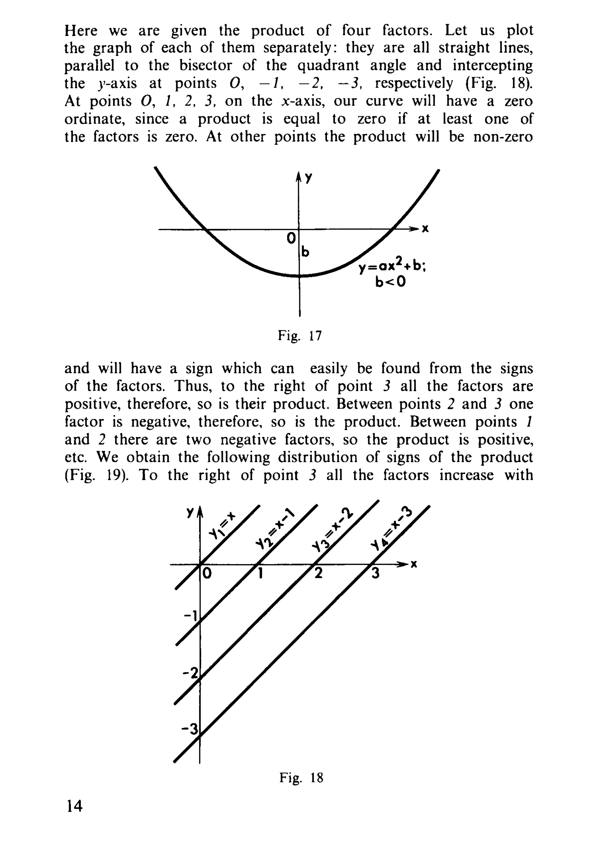
(b) When multiplying graphs pay attention to the points where
factors (at least one of them) become zero; remember the rule of
signs between those points.
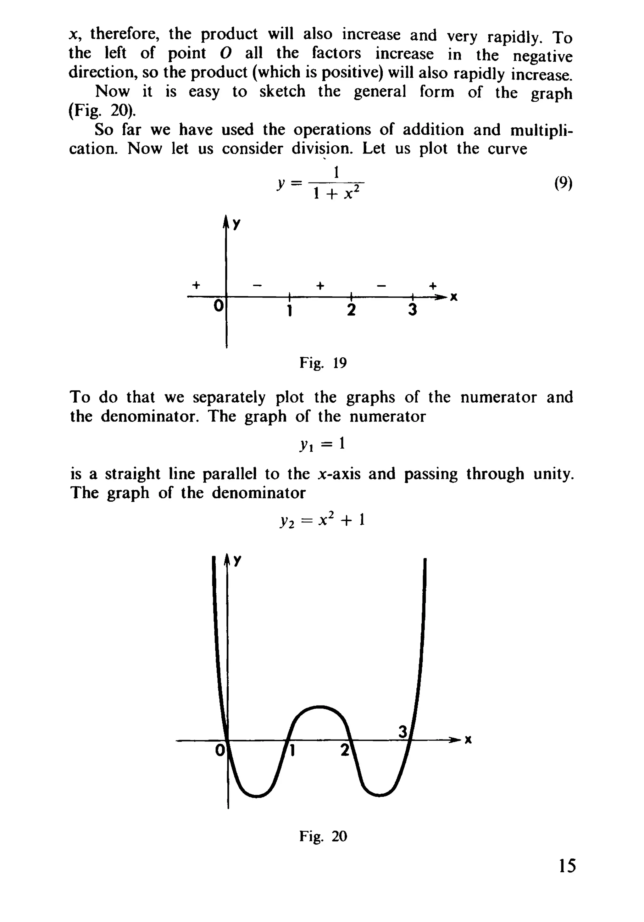
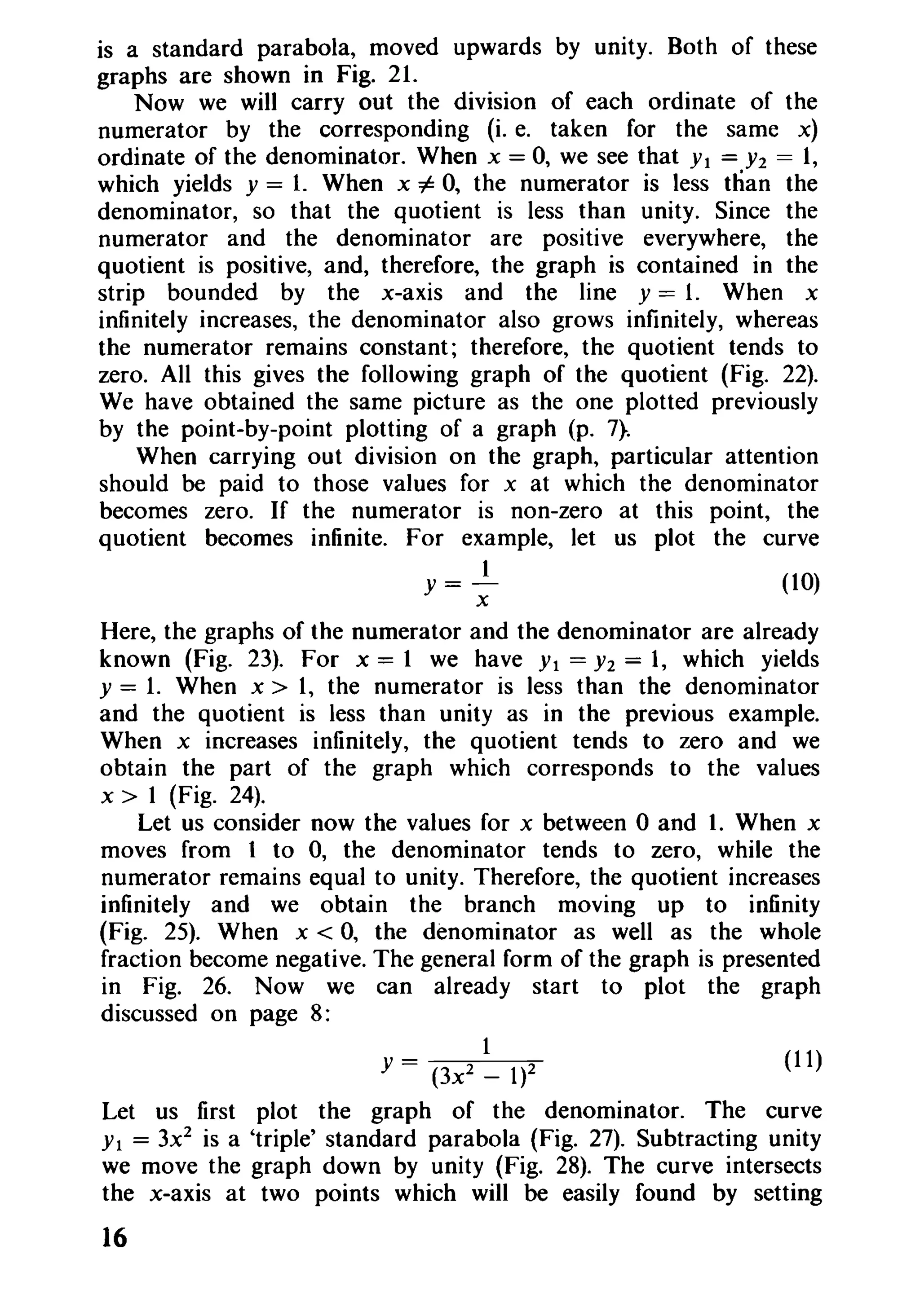
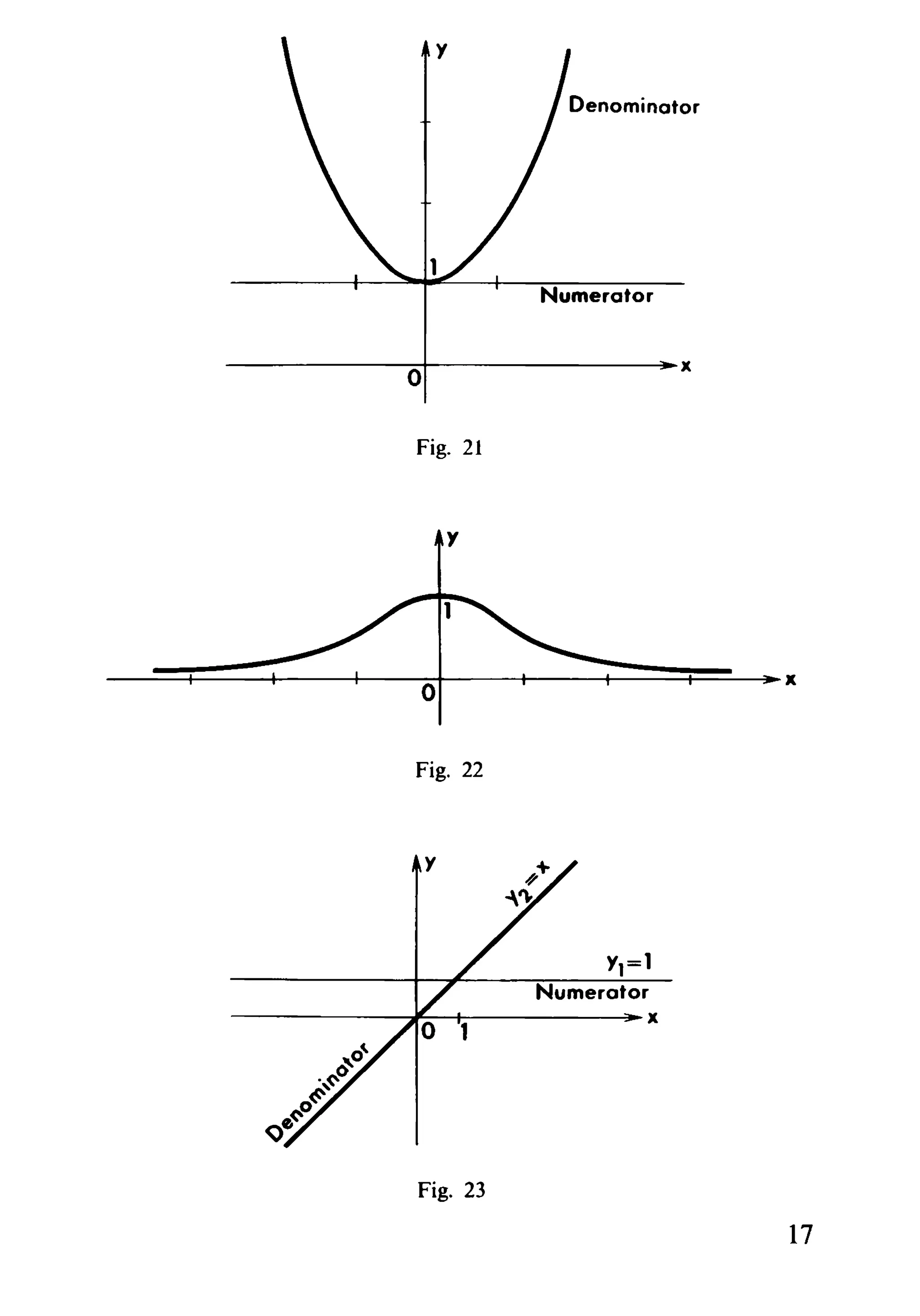
(c) When dividing graphs pay attention to the points where
denominator vanishes. If at those points numerator is non-zero,
the branches of the curve will move to infinity - up or down
depending on the signs of the numerator and the denominator.
(d) Pay attention to the behaviour of the curve when x
moves indefinitely to the right (to +(0) or to the left (to - oo].
Here we have only described the simplest operations which
may be carried out with graphs. To be more precise, we started
out with the simplest equation y = x and applied further the four
operations of arithmetic: addition, subtraction, multiplication, and
division. To these operations we could easily add the algebraic
operation - extracting roots.
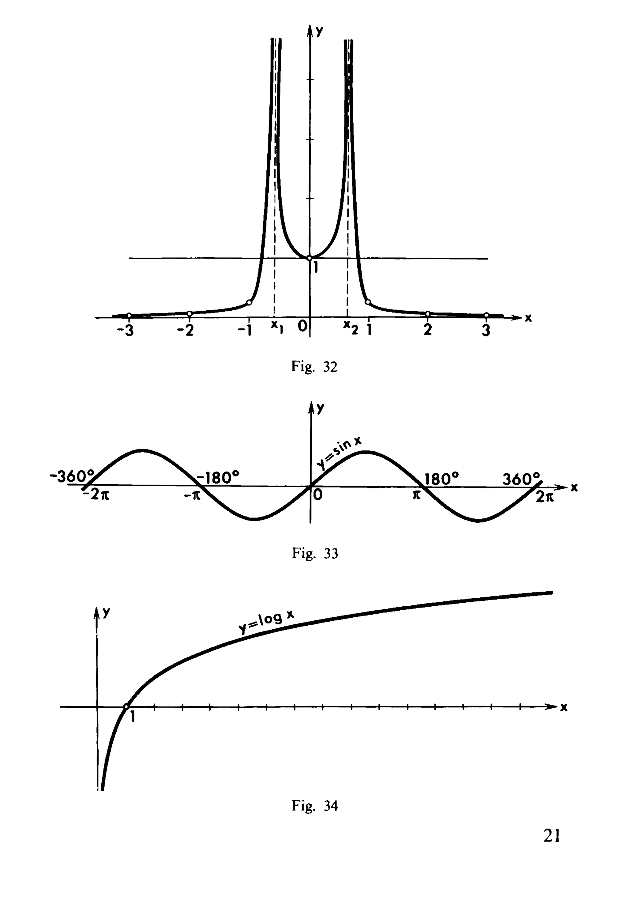
But more complicated operations - trigonometric and logarithmic
ones - can also be carried out with graphs. One only needs to
know the graphs of the simplest equations y = sin x (Fig. 33)
and y = logx (Fig. 34). Using the methods desribed above we can
plot graphs of any equations involving the symbols sin, log,
and algebraic and arithmetic operations.
It is very useful to learn how to plot all kinds of graphs.
However, by using the methods indicated above we will not be
able to answer many natural questions arising when one considers
some graphs. For example, we see on a certain graph that the
curve rises to some value Yo, then begins to move down; we say
in that case that it reaches its maximum value Yo at point Xo.
We may not be able to find the exact value of Xo with our
limited scope of methods. Other questions arise, for example, at
what angle the curve intersects the x- or the y-axis, whether it
22
25. is convex upward or downward. Our methods cannot give exact
answers to all of those questions. Here, a considerably more
serious knowledge of mathematical technique is required. The
methods which allow the study of the above properties of graphs
are contained in the branch of mathematics known as the differential
calculus.
*
* *
In conclusion solve some problems on graphs.
Plot the graphs of the following equations:
1. y = x2
+ X + 1. 3. y = x2
(x - 1).
2. y = x(x2
- 1).
x
5. Y=--l.
x-
4. y = x(x - 1)2
x 1
Hint. Single out the integral part: ---= 1 + --.x-I x-I
x2
6. y= --1.
x-
Hint. Single out the integral part.
x 3
7. y = --1-.
'x-
Hint. Single out the integral part.
8. y = ± ~.
Hint. The square root of negative numbers does not exist In
the real part.
9.y=±~
How to prove that this curve is a circle?
Hint. Recall the definition of a circle and the Pythagorean
theorem.
1ft y=±~.
23
26. Prove that the upper branch of the curve indefinitely approaches
the bisector of the quadrant angle when x ~ 00.
Hint. Vx2
+ 1 - x == 1
~+x·
11. y= ±xVx(l-x).
12. y= ±X2~.
13. y= 1~.
2 ± V1 - x2
14. Y == x 2/3 (1 - x)2/3 .
32. Recommended Literature
The Encyclopedia of Elementary Mathematics, Book 3, Gostekhizdat
(19.52), the article by V. L. Goncharov "Elementary Functions", Chaps.
1 and 2.
33. TO THE READER
Mir Publishers welcome your comments on the content,
translation and design of this book.
We would also be pleased to receive any proposals you
care to make about our future publications.
Our address is:
USSR., 129820., Moscow, 1-110, GSP
Pervy Rizhsky Pereulok, 2
Mir Publishers
Printed in the Union of Soviet Socialist Republics