The document discusses Binary Decision Diagrams (BDDs) and Ordered BDDs (OBDDs) which provide a more compact representation of Boolean functions compared to truth tables. It describes algorithms for reducing, applying logical operations, restricting variables, and checking satisfiability on BDDs/OBDDs. OBDDs ensure variables appear in the same order on all paths, allowing efficient equivalence checking. The document concludes with applications of OBDDs in symbolic model checking where sets of states are represented as OBDDs.

1. Binary Decision Diagrams
Presenter: Haroon Rashid
1
11/21/2014

2. Contents
Motivation
Binary Decision Diagrams (BDDs)
Ordered BDDs
Reduced OBDD algorithms
reduce
apply
restrict
exists
Applications of OBDDs
2
11/21/2014

3. Motivation: Boolean Function Representation
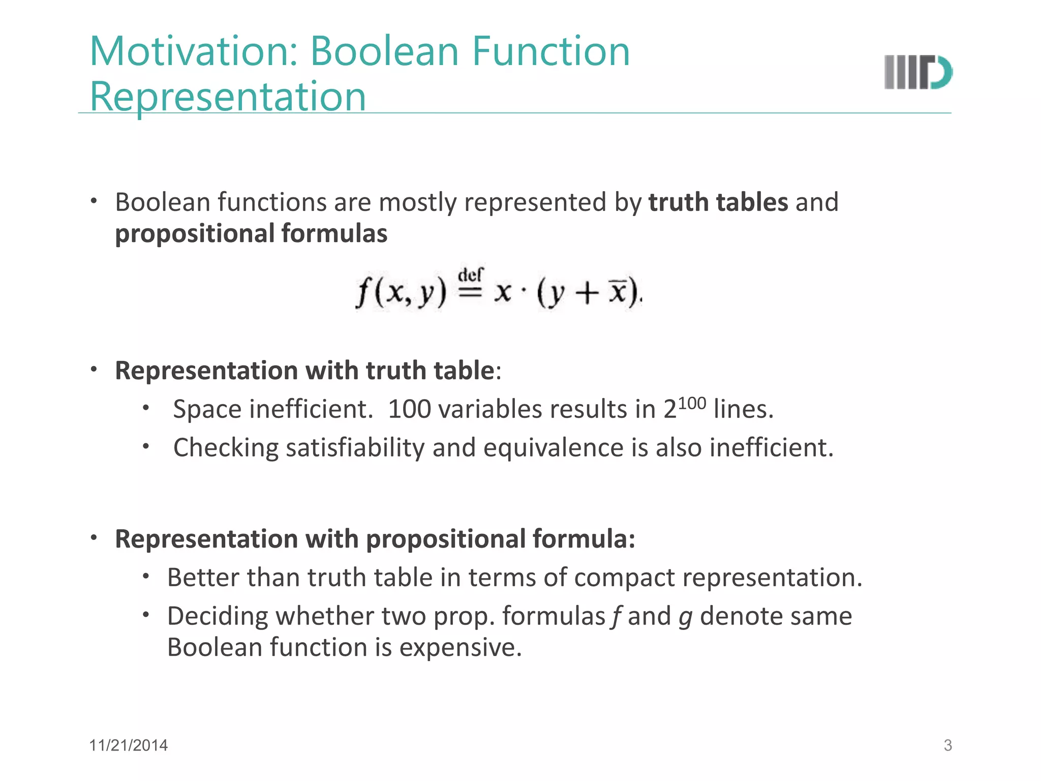
Boolean functions are mostly represented by truth tables and propositional formulas
Representation with truth table:
 Space inefficient. 100 variables results in 2100 lines.
 Checking satisfiability and equivalence is also inefficient.
Representation with propositional formula:
Better than truth table in terms of compact representation.
Deciding whether two prop. formulas f and g denote same Boolean function is expensive.
3
11/21/2014

4. Binary Decision Diagrams (BDDs)
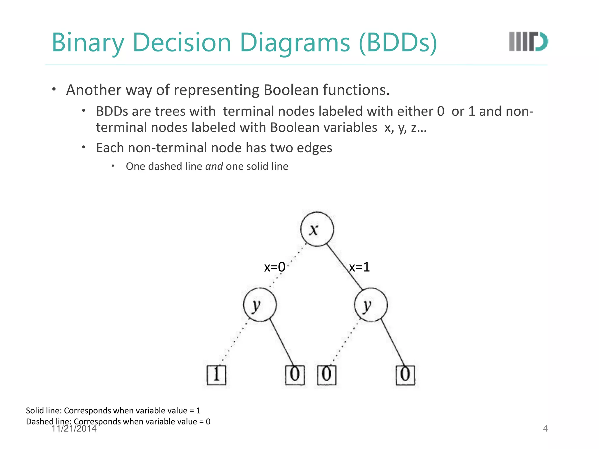
Another way of representing Boolean functions.
BDDs are trees with terminal nodes labeled with either 0 or 1 and non- terminal nodes labeled with Boolean variables x, y, z…
Each non-terminal node has two edges
One dashed line and one solid line
4
x=0
x=1
Solid line: Corresponds when variable value = 1 Dashed line: Corresponds when variable value = 0
11/21/2014

5. BDD functions
5
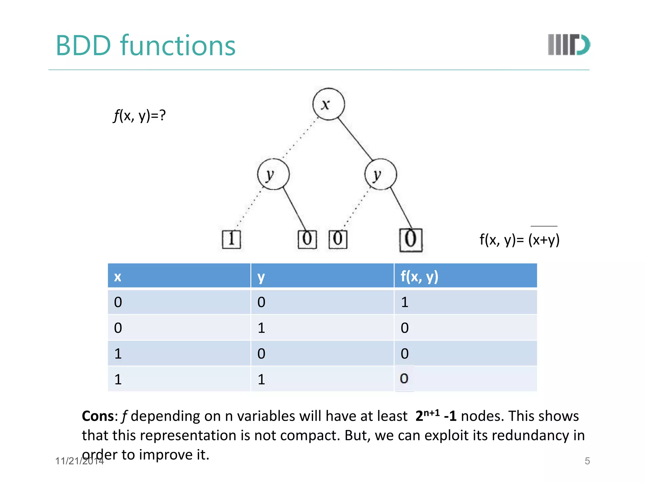
f(x, y)=?
x
y
f(x, y)
0
0
1
0
1
0
1
0
0
1
1
1
f(x, y)= (x+y)
Cons: f depending on n variables will have at least 2n+1 -1 nodes. This shows that this representation is not compact. But, we can exploit its redundancy in order to improve it.
11/21/2014

6. BDD Contraction
6
•[C1]: Removal of duplicate terminals
•[C2]: Removal of redundant tests
•[C3]: Removal of duplicate non-terminals
Duplicate Terminals
Duplicate Non-terminals Terminals
11/21/2014

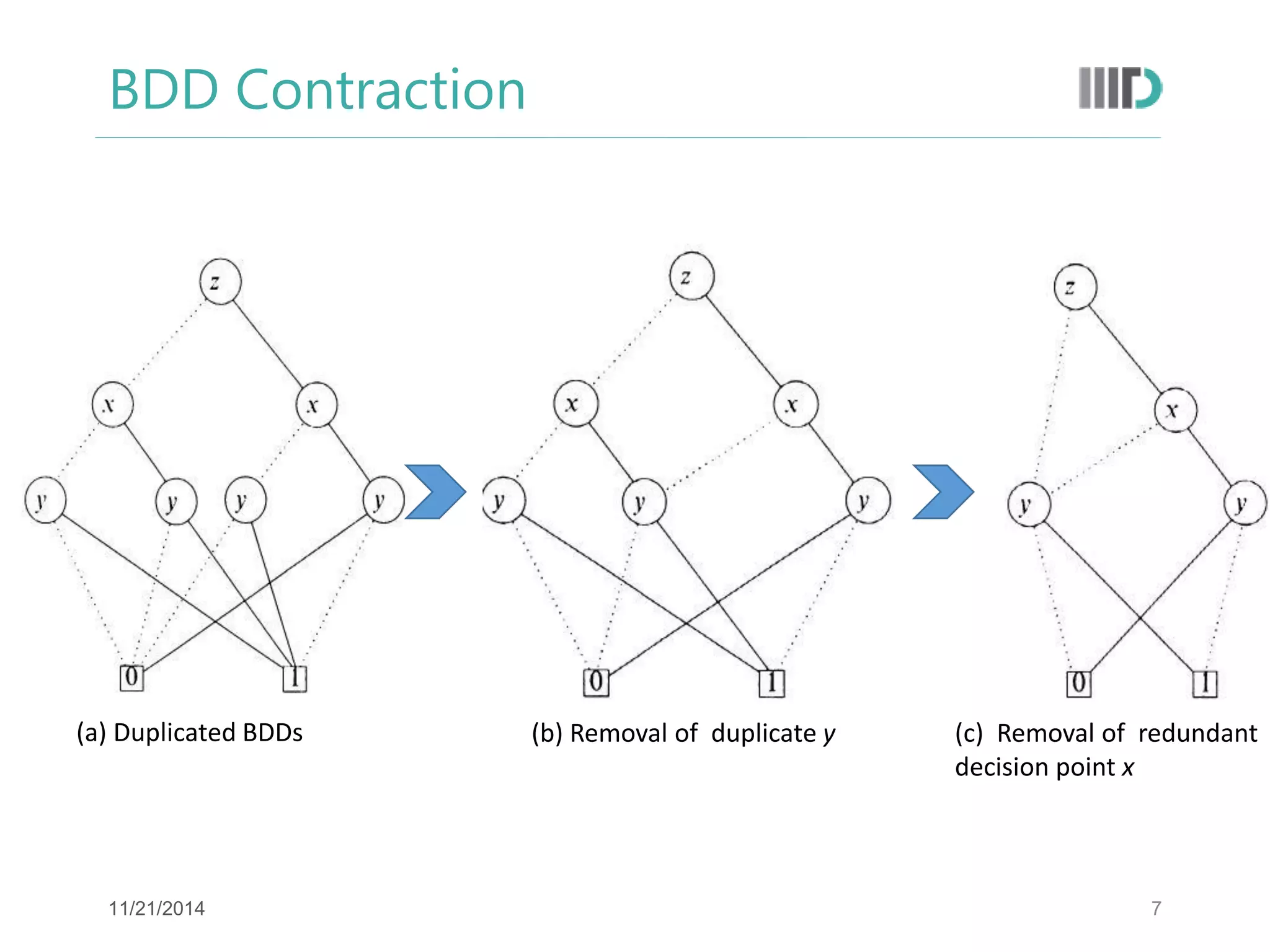
7. BDD Contraction
7
(a) Duplicated BDDs
(b) Removal of duplicate y
(c) Removal of redundant decision point x
11/21/2014

8. Satisfiability, Validity and operations (.,+)
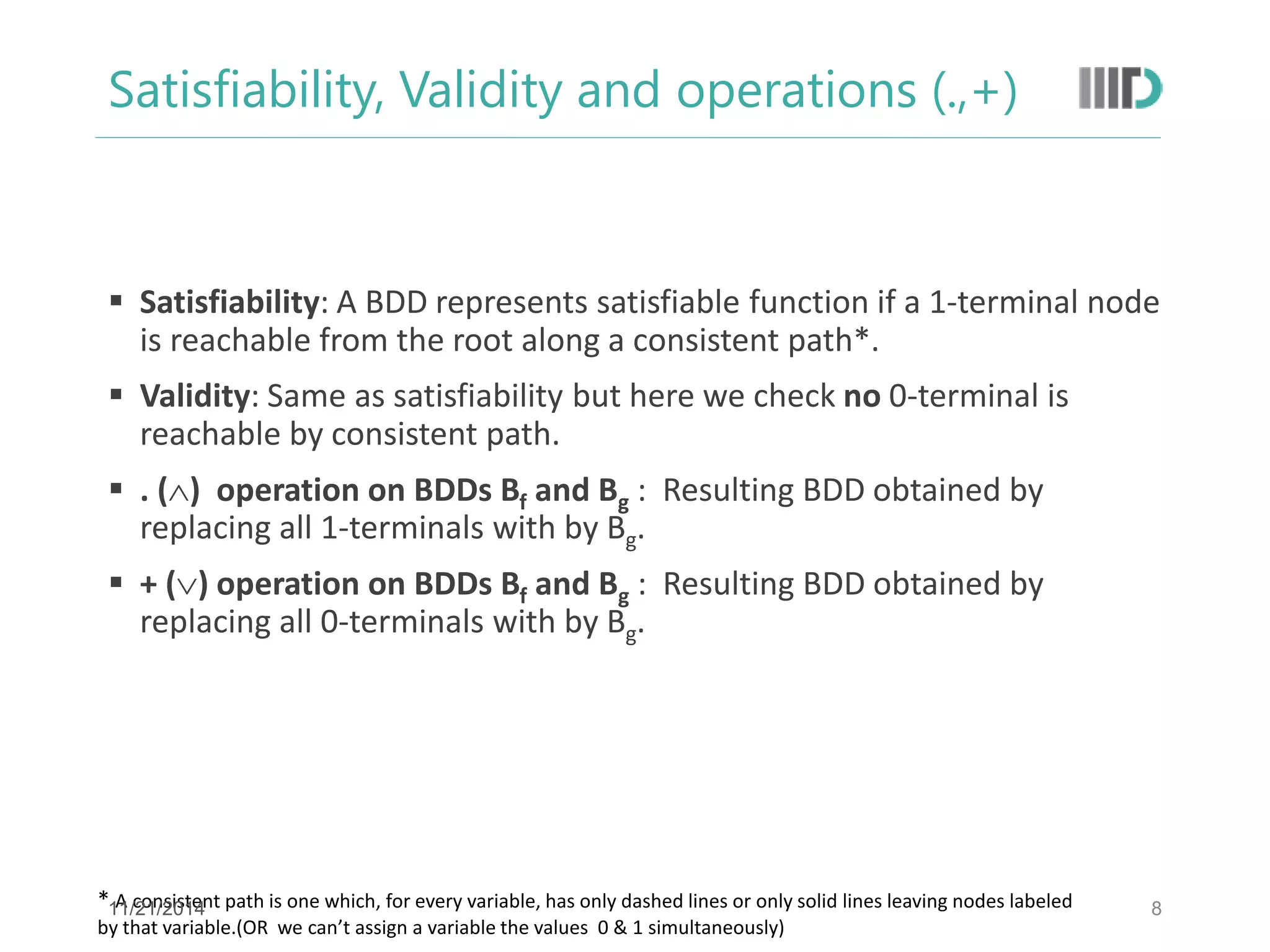
Satisfiability: A BDD represents satisfiable function if a 1-terminal node is reachable from the root along a consistent path*.
Validity: Same as satisfiability but here we check no 0-terminal is reachable by consistent path.
. () operation on BDDs Bf and Bg : Resulting BDD obtained by replacing all 1-terminals with by Bg.
+ () operation on BDDs Bf and Bg : Resulting BDD obtained by replacing all 0-terminals with by Bg.
8
* A consistent path is one which, for every variable, has only dashed lines or only solid lines leaving nodes labeled by that variable.(OR we can’t assign a variable the values 0 & 1 simultaneously)
11/21/2014

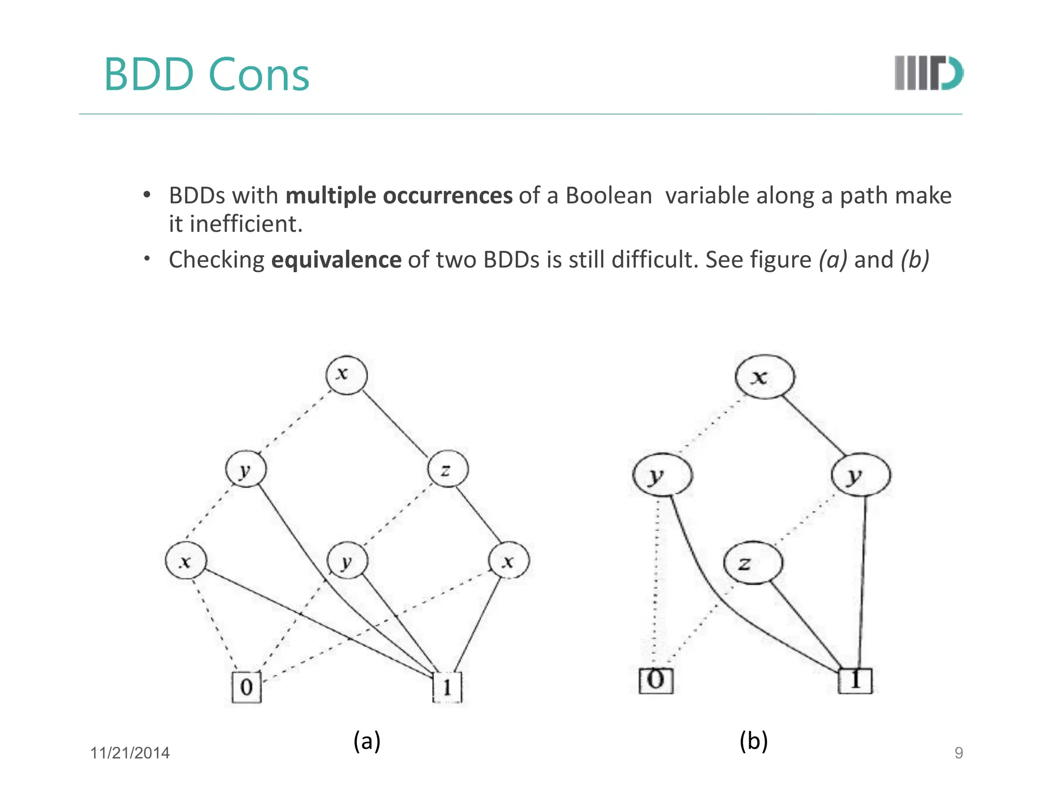
9. BDD Cons
•BDDs with multiple occurrences of a Boolean variable along a path make it inefficient.
Checking equivalence of two BDDs is still difficult. See figure (a) and (b)
9
(a)
(b)
11/21/2014

10. Ordered BDDs
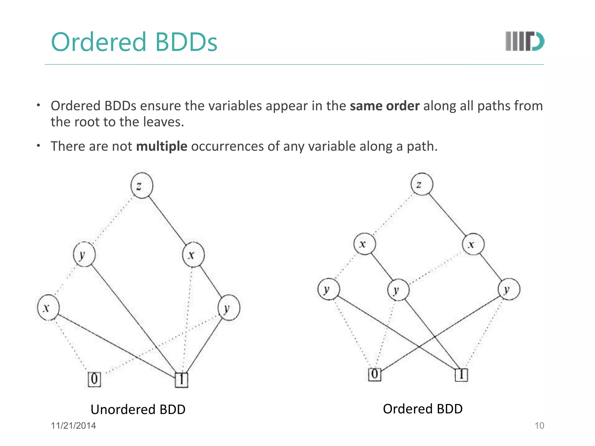
Ordered BDDs ensure the variables appear in the same order along all paths from the root to the leaves.
There are not multiple occurrences of any variable along a path.
10
Unordered BDD
Ordered BDD
11/21/2014

11. Ordered BDDS cont..
With OBDDs we cannot have more than one BDD representing the same function, i.e., one function -> one OBDD.
Follows that checking equivalence with OBDDs is immediate.
OBDDS for f = (x1+x2 ). (x3+x4 ). (x5+x6 )
11
Ordering: [x1, x2, x3, x4, x5, x6 ]
Ordering: [x1, x3, x5, x2, x4, x6 ]
11/21/2014

12. Reduced OBDDs Algorithm: reduce
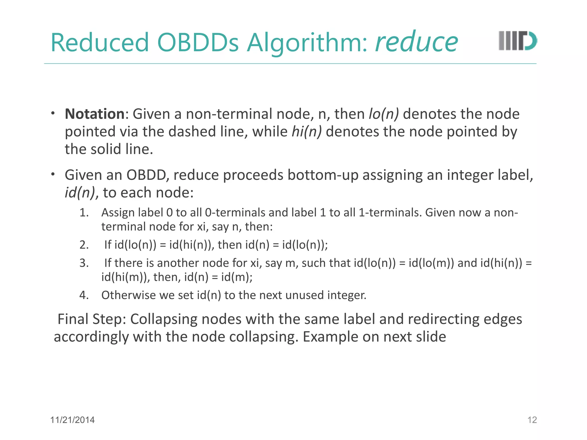
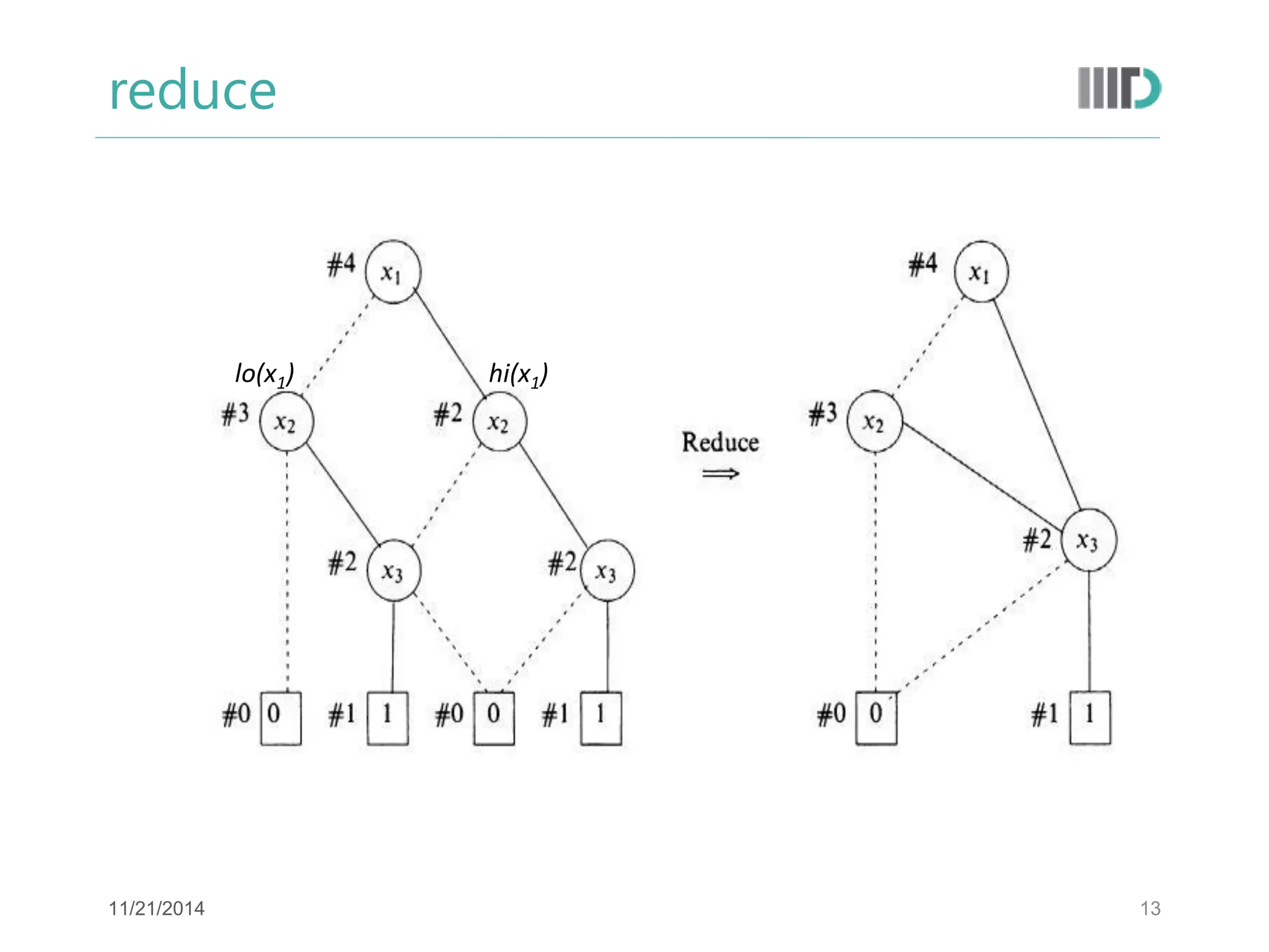
Notation: Given a non-terminal node, n, then lo(n) denotes the node pointed via the dashed line, while hi(n) denotes the node pointed by the solid line.
Given an OBDD, reduce proceeds bottom-up assigning an integer label, id(n), to each node:
1.Assign label 0 to all 0-terminals and label 1 to all 1-terminals. Given now a non- terminal node for xi, say n, then:
2. If id(lo(n)) = id(hi(n)), then id(n) = id(lo(n));
3. If there is another node for xi, say m, such that id(lo(n)) = id(lo(m)) and id(hi(n)) = id(hi(m)), then, id(n) = id(m);
4.Otherwise we set id(n) to the next unused integer.
Final Step: Collapsing nodes with the same label and redirecting edges accordingly with the node collapsing. Example on next slide
12
11/21/2014

13. reduce
13
lo(x1)
hi(x1)
11/21/2014

14. Algorithm apply
apply is used to implement operations like ., + on Boolean functions
Definition: Let β be a formula and x a variable. We denote by β[0/x] (β[1/x]) the formula obtained by replacing all occurrences of x in β by 0 (1).
Lemma [Shannon Expansion]: Let β be a formula and x a variable, then:
β = x . β[0/x] + x. β[1/x]
The function apply is based on Shannon Expansion for α op β :
α op β = x. (α .[0/x] op β[0/x] ) + x. (α .[1/x] op β[1/x] )
14
11/21/2014

15. Algorithm apply
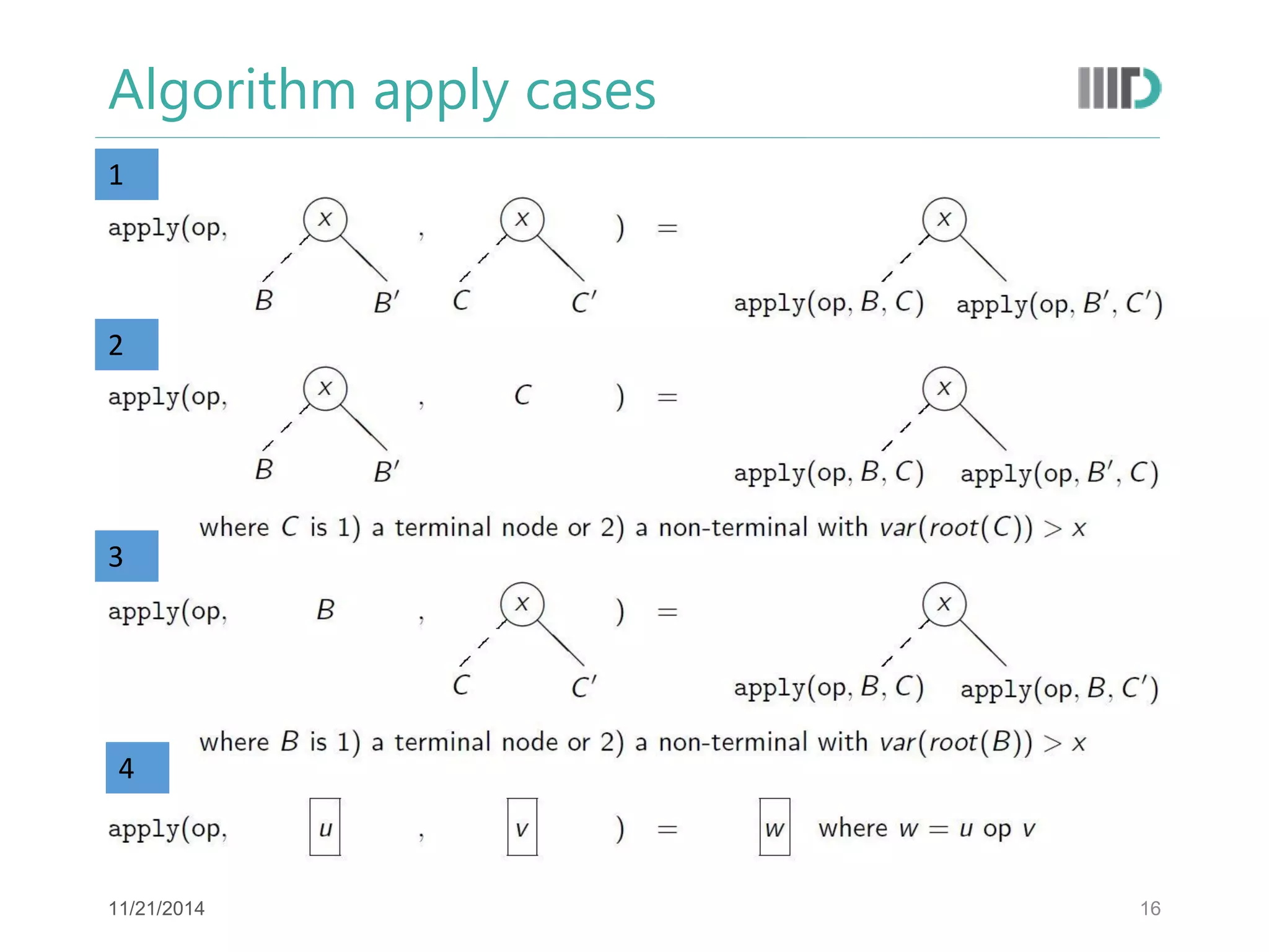
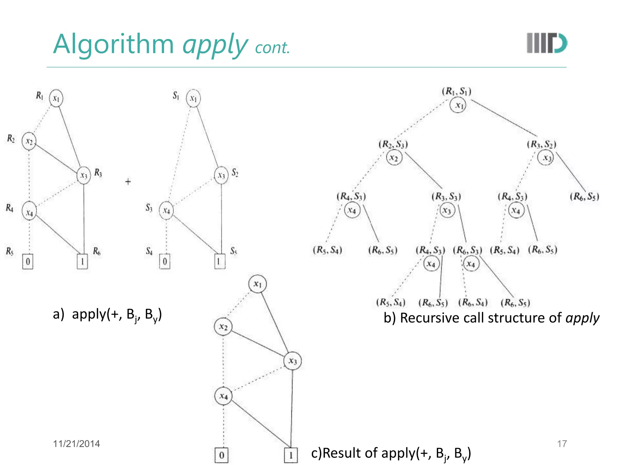
apply (op, Bj, By) proceeds from the roots downward.
Let rj, ry be the roots of Bj, By respectively:
 If both rj, ry are terminal nodes, then,
apply(op, Bj, By) = B(rj op ry)
If both roots are xi-nodes, then create an xi-node with a dashed line to apply(op, Blo(rj), Blo(ry)) and a solid line to apply(op, Bhi(rj), Bhi(ry))
If rj is an xi-node, but ry is a terminal node or an xj-node with j > i (i.e., y[0/xi] ≡ y[1/xi] ≡ y), then create an xi-node with dashed line to
apply(op, Blo(rj), By) and solid line to apply(op, Bhi(rj), By)
If ry is an xi-node, but rj is a terminal node or an xj-node with j > i, is handled as above.
15
11/21/2014

16. Algorithm apply cases
16
1
2
3
4
11/21/2014

17. Algorithm apply cont.
17
a) apply(+, Bj, By)
b) Recursive call structure of apply
c)Result of apply(+, Bj, By)
11/21/2014

18. Algorithm restrict
Given an OBDD Bf representing Boolean formula f, algorithm restrict(0, x, Bf) computes reduced OBDD representing f [0/x] as:
 Bf[0/x] = restrict(0, x, Bf).
For each node n labeled with x, then:
1. Incoming edges are redirected to lo(n)
2. n is removed.
 Bf[1/x] = restrict(1, x, Bf).
Same as above, but redirecting incoming edges to hi(n)
18
11/21/2014

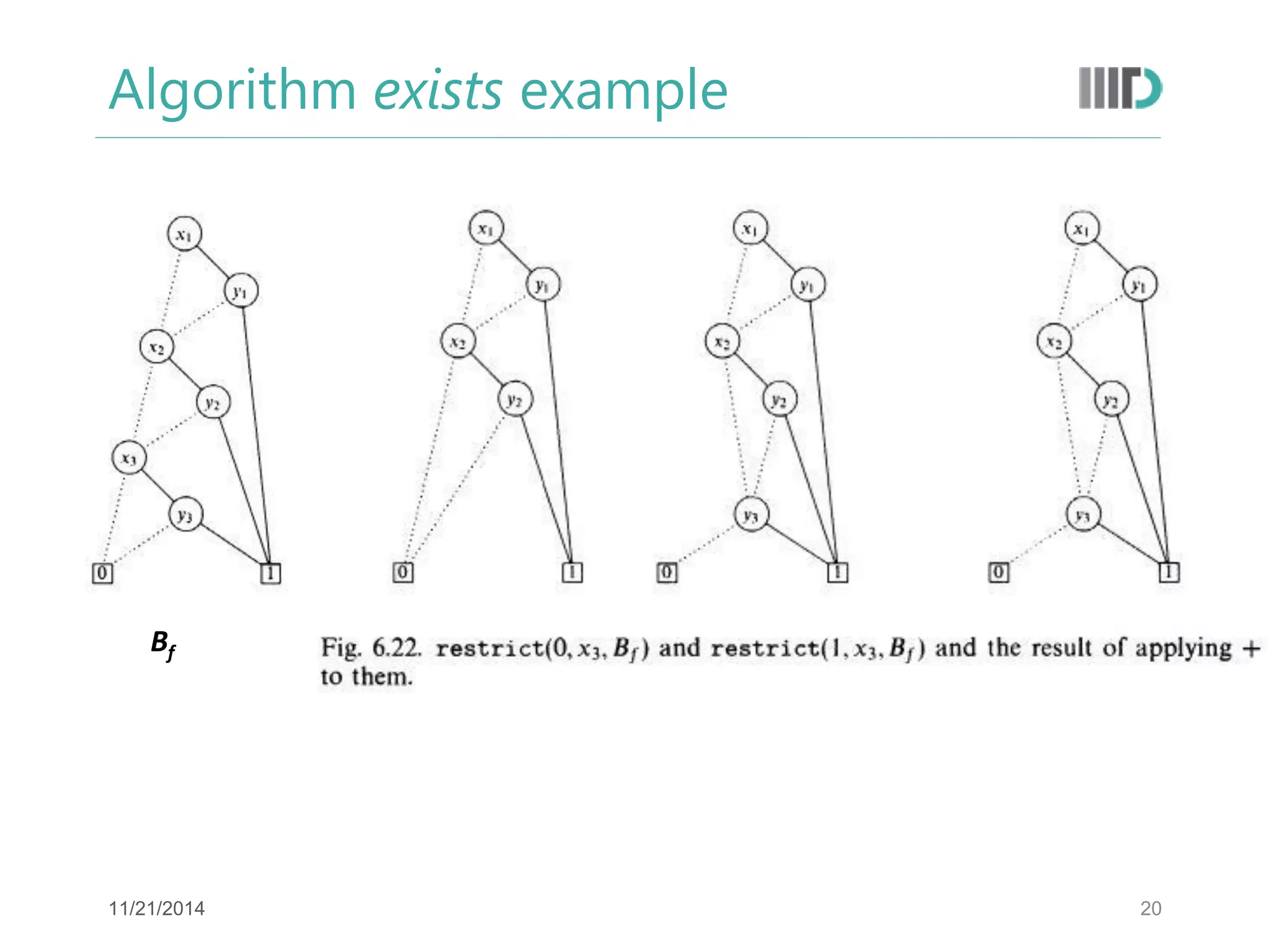
19. Algorithm exists [apply+restrict]
exists is used to perform operation on Boolean function while relaxing constraint on some variable.
We write (∃x. ƒ) for the Boolean function ƒ with the constraint on x relaxed and it can be expressed as:
∃x. ƒ = ƒ [0/x]+ ƒ[1/x]
i.e., there exists x on which the constraint is relaxed
The exists algorithm can be implemented in terms of algorithms apply and restrict as
∃x. ƒ = apply(+, restrict(0, x, Bf), restrict(1, x, Bf))
19
11/21/2014

20. Algorithm exists example
20
Bf
11/21/2014

21. OBDDs Application
Symbolic Model Checking
Model checking using OBDDs is called symbolic model checking
OBDDs allow systems with a large space to be verified.
Normally, Labeling algorithm takes a CTL formula and returns a set of states manipulating intermediate set of states.
The algorithm is changed by storing set of states as OBDD's and then manipulating them.
21
11/21/2014

22. Symbolic Representation
Three states X1, X2, X3:
{000,001,010,011} represented as first bit false: ┐X1
With five state variables X1, X2, X3, X4, X5:
{00000,00001,00010,00011,00100,00101,00110, 00111, ,…, 01111} still represented as first bit false: ┐X1
22
11/21/2014

23. Conclusion
BDDs and OBDDs
Application of various algorithms
Application of OBDDs in model checking
23
11/21/2014

24. References
Logics in Computer Science, Modelling and Reasoning about Systems, Chapter 6, M. Huth and M. Ryan.
Slides of Alessandro Artale, http://www.inf.unibz.it/~artale/FM/slide7.pdf
24
11/21/2014

25. Questions ?
25
11/21/2014