Download as PDF, PPTX


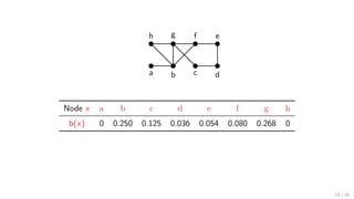
![Domain Knowledge / Modeling: Assume that
1) every node wants to communicate with every node; and
2) communication progresses along Shortest Paths (SPs).
Then, the higher the no. of SPs that a node v belongs to, the more important v is.
Definition
For each node x ∈ V , the betweeness b(x) of x is:
b(x) =
1
n(n − 1) u=x=v∈V
σuv (x)
σuv
∈ [0, 1]
• σuv : number of SPs from u to v, u, v ∈ V ;
• σuv (x): number of SPs from u to v that go through x.
I.e., b(x) is weighted fraction of SPs that go through x, among all SPs in G.
13 / 24](https://image.slidesharecdn.com/riondato-algorithmicdatascience-mitu-slides-180723155908/85/Algorithmic-Data-Science-Theory-Practice-18-320.jpg)


![Theory + Practice:
Get rid of “theoretical elegance” while maintaining correctness.
Let
gS(x, y) = 2 exp −2 x2
(y − 2RF (S))2
+ exp − ((1 − x)y + 2xRF (S))
φ
2RF (S)
(1 − x)y + 2xRF (S)
− 1 .
Then compute
min
x,ξ
ξ
s.t. gS(x, ξ) ≤ η
ξ ∈ (2RF (S), 1]
x ∈ (0, 1)
and check if ξ < ε.
21 / 24](https://image.slidesharecdn.com/riondato-algorithmicdatascience-mitu-slides-180723155908/85/Algorithmic-Data-Science-Theory-Practice-43-320.jpg)


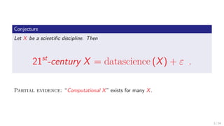
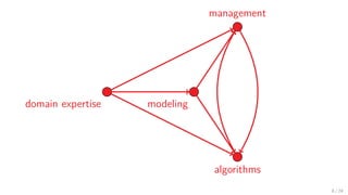
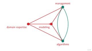
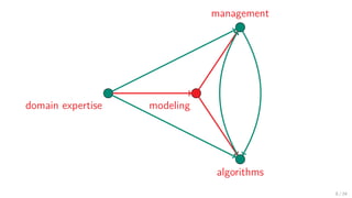
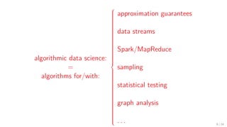
The document discusses the concept of algorithmic data science, which combines theoretical and practical approaches in the field of data science. It emphasizes the necessity of domain expertise, mathematical modeling, and algorithms to solve various scientific questions while proposing methods for efficient data representation and approximations. Additionally, it highlights the importance of sampling techniques for achieving probabilistic approximations in graph analysis.