The document provides a comprehensive guide on query tuning in PostgreSQL, detailing essential commands for diagnosis, execution plans, and optimization techniques. It explains the importance of various system and database settings that affect query performance, as well as the methodology for interpreting execution plans. Additionally, it discusses common pitfalls in query design and how to refine queries for improved efficiency.

1. Basic Query Tuning Primer Pg West 2009 2009-10-17

2. Basic tool kit for query tuning For Diagnosis: EXPLAIN and EXPLAIN ANALYZE

3. Query pg_class

4. Query pg_stats

5. SET enable_[nestloop|hashagg|...] = [on|off]

6. SET [random_page|...]_cost = [n]

7. RESET all

8. Postgres server logs May need to adjust log_* GUCS such as: log_temp_files, log_lock_waits, log_min_duration_statement, log_checkpoints, log_statement_stats, etc. auto_explain (new contrib module in Pg 8.4)

9. Occasionally helpful: gdb, dtrace, sar, iostat -x, etc. For Remedy: ANALYZE [table]

10. ALTER TABLE [table] ALTER COLUMN [column] SET STATISTICS [n]

11. SET default_statistics_target = [n], work_mem = [n]

12. CREATE INDEX

13. Reorganize the SQL (e.g. filter large tables directly, avoid joins, refactor to temp tables or WITH clause, etc.)

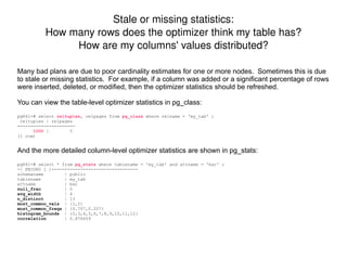
14. Rarely appropriate: SET [gucs], table-level autovac storage-params, denormalize columns, partition large table

15. System tuning is not query tuning Relevance: System tuning affects all queries, but it optimizes for an aggregate workload, not an individual query. The overall performance of a system is the product of many factors, including but not limited to: Hardware platform: cpu speed/count, memory speed/amount, disk type/count, raid layout, controller model

16. System settings: kernel cache page size, tcp buffer size, dirty page flush policy, io scheduler, etc.

17. Filesystem settings: type, readahead, direct/buffered io, extent size, journaling policy, internal/external journal, atime/mtime maint., existence of snapshots, etc.

18. Postgres settings: version, GUCS (default_statistics_target, shared_buffers, temp_buffers, work_mem, wal_buffers, *_cost, enable_*, effective_cache_size, fsync), WAL on separate disks, etc.

19. Total workload: cumulative effect of all tasks running at a particular point in time, all of which compete for resources (e.g. cpu, memory, cache, disk I/O, locks).

20. Accumulated state: contents of caches (Pg, kernel, controller), physical file fragmentation on disk, optimizer statistics (specific to cluster; not portable via pg_dump)

21. What is an execution plan? To see a query's execution plan, use the EXPLAIN command before the query. To also run the query and capture how much time was spent in each step of the plan, use EXPLAIN ANALYZE . Original SQL: pg841=# select count(*) from orders where created_ts >= '2009-09-01'::timestamp ; count ------- 65472 (1 row) Execution plan with estimated costs and row-counts: pg841=# explain select count(*) from orders where created_ts >= '2009-09-01'::timestamp ; QUERY PLAN ------------------------------------------------------------------------------------ Aggregate (cost=2100.85..2100.86 rows=1 width=0) -> Seq Scan on orders (cost=0.00..1937.00 rows= 65538 width=0) Filter: (created_ts >= '2009-09-01 00:00:00'::timestamp without time zone) (3 rows) Execution plan with actual runtimes and row-counts: pg841=# explain analyze select count(*) from orders where created_ts >= '2009-09-01'::timestamp ; QUERY PLAN ------------------------------------------------------------------------------------------------------------------- Aggregate (cost=2100.85..2100.86 rows=1 width=0) (actual time=251.210..251.212 rows=1 loops=1) -> Seq Scan on orders (cost=0.00..1937.00 rows= 65538 width=0) (actual time=0.018..140.495 rows= 65472 loops=1) Filter: (created_ts >= '2009-09-01 00:00:00'::timestamp without time zone) Total runtime: 251.269 ms (4 rows)

22. Each step in the execution plan is a node in a tree hierarchy. The leftmost (“top”) node pulls data from its children, which do the same for their children. Nodes with no children start working first, since they gather the data from tables or indexes to be processed by the rest of the plan nodes. Run Order QUERY PLAN ------- --------------------------------------------------------------------------------------------------------------- 4th HashAggregate (cost= 1119.28 ..1120.75 rows=98 width=12) 3rd -> Nested Loop (cost= 0.00 ..1118.79 rows=98 width=12) 1st -> Index Scan using idx_order_details_product_id on order_details (cost= 0.00 ..397.99 rows=98 width=8) Index Cond: (product_id = 1000) 2nd -> Index Scan using orders_pkey on orders (cost= 0.00 ..7.34 rows=1 width=12) Index Cond: (orders.order_id = order_details.order_id) Filter: (orders.created_ts >= '2009-09-01 00:00:00'::timestamp without time zone) (7 rows) Reading an execution plan: In what order do the nodes run?

23. The two numbers for “cost” and “actual time” represent when the 1st and last rows will be output by that node. Different kinds of nodes have different amounts of lag between when it receives its first input and when it produces its first output. This “startup cost” is implied by the difference in the first cost value of the node vs. its slowest-starting child . Here, the Hash node has high startup cost – it cannot feed data to its parent ( Hash Join ) until it receives and processes all of the data from its child Seq Scan node. So the Seq Scan node's final cost ( 1937.00 ) becomes the Hash node's initial cost ( 1937.00 ). In practice, the child's actual completion time ( 151.703 ) is a lower bound for the Hash node's first-output time ( 288.962 ). QUERY PLAN ------------------------------------------------------------------------------------------------------------------------- Hash Join ( cost= 3013.22 .. 45974.93 rows=651270 width=12) ( actual time= 289.152 .. 6297.282 rows=654720 loops=1) Hash Cond: (order_details.order_id = orders.order_id) -> Seq Scan on order_details ( cost= 0.00 .. 14902.00 rows=1000000 width=12) ( actual time= 0.037 .. 2026.802 rows=1000000 loops=1) -> Hash ( cost= 1937.00 .. 1937.00 rows=65538 width=8) ( actual time= 288.962 .. 288.962 rows=65472 loops=1) -> Seq Scan on orders ( cost= 0.00 .. 1937.00 rows=65538 width=8) ( actual time= 0.014 .. 151.703 rows=65472 loops=1) Filter: (created_ts >= '2009-09-01 00:00:00'::timestamp without time zone) Total runtime: 7349.662 ms (7 rows) Reading an execution plan: What do the numbers mean for "cost" and "actual time"?

24. Access methods are used by leaf nodes to pull data from tables/indexes. Join methods specify which type of algorithm will be used to implement each of the query's joins. QUERY PLAN ------------------------------------------------------------------------------------------------------ Sort (cost=248.54..248.79 rows=99 width=8) Sort Key: o.order_id -> Nested Loop (cost=4.34..245.26 rows=99 width=8) -> Nested Loop (cost=4.34..234.94 rows=10 width=4) -> Seq Scan on customers c (cost=0.00..194.00 rows=1 width=4) Filter: (name = 'JOHN DOE'::text) -> Bitmap Heap Scan on orders o (cost=4.34..40.82 rows=10 width=8) Recheck Cond: (o.cust_id = c.cust_id) -> Bitmap Index Scan on idx_orders_cust_id (cost=0.00..4.34 rows=10 width=0) Index Cond: (o.cust_id = c.cust_id) -> Index Scan using order_details_pk on order_details od (cost=0.00..0.91 rows=10 width=8) Index Cond: (od.order_id = o.order_id) (12 rows) QUERY PLAN ---------------------------------------------------------------------------------------------------------------------- Aggregate (cost=18850.37..18850.38 rows=1 width=8) -> Hash Join (cost=53.18..18801.97 rows=9679 width=8) Hash Cond: (od.order_id = o.order_id) -> Seq Scan on order_details od (cost=0.00..14902.00 rows=1000000 width=8) -> Hash (cost=41.00..41.00 rows=974 width=4) -> Index Scan using pidx_orders_order_id_not_shipped on orders o (cost=0.00..41.00 rows=974 width=4) Filter: is_paid (7 rows) Reading an execution plan: What are access methods and join methods?

25. Create and ANALYZE a small toy table. pg841=# create temp table my_tab1 as select * from orders limit 100 ; SELECT pg841=# analyze my_tab1 ; ANALYZE EXPLAIN a simple query against it. pg841=# explain select * from my_tab1 where created_ts > '2009-10-14 08:14:26'::timestamp - '1 day'::interval ; QUERY PLAN ------------------------------------------------------------------------------------ Seq Scan on my_tab1 (cost=0.00.. 2.25 rows=17 width=25) Filter: (created_ts > '2009-10-13 08:14:26' ::timestamp without time zone) (2 rows) The planner was able to combine the filter's two literals. The table is accessed by SeqScan, since there are no indexes yet on this temp table. Add an index, force the planner not to SeqScan, and compare the same query's cost estimates for IndexScan versus SeqScan. pg841=# create index idx_my_tab1_test on my_tab1 ( created_ts ) ; CREATE INDEX pg841=# set enable_seqscan = off ; SET pg841=# explain select * from my_tab1 where created_ts > '2009-10-14 08:14:26'::timestamp - '1 day'::interval ; QUERY PLAN ---------------------------------------------------------------------------------------- Index Scan using idx_my_tab1_test on my_tab1 ( cost =0.00.. 8.55 rows=17 width=25) Index Cond: (created_ts > '2009-10-13 08:14:26'::timestamp without time zone) (2 rows) pg841=# reset all ; RESET The optimizer prefers (assigns a lower cost) to SeqScan this table because it is so tiny (1 block). An IndexScan would require reading a 2nd block (the index itself) and doing extra comparisons. Play with small toy queries.

26. Run your query with EXPLAIN (or if practical, EXPLAIN ANALYZE), and look for nodes where the cost, row-count, or actual_time significantly increases compared to its children. In this example, the SQL is missing its join criteria. The estimated cost and row-count skyrocket in the Nested Loop node, because it is returning the cross-product of all rows from both its input nodes. pg841=# explain pg841-# select pg841-# customers.cust_id as customer_id, pg841-# max(customers.name) as customer_name, pg841-# count(distinct orders.order_id) as num_orders, pg841-# max(orders.shipped_ts) as latest_shipment_datetime pg841-# from orders, customers , products /* THIS JOIN TO “products” IS SPURIOUS */ pg841-# where pg841-# orders.cust_id = customers.cust_id pg841-# and orders.created_ts >= now() - '30 days'::interval pg841-# group by pg841-# customers.cust_id pg841-# order by num_orders desc pg841-# limit 10 pg841-# ; QUERY PLAN ----------------------------------------------------------------------------------------------------------------------- Limit ( cost =15307415.27.. 15307415.29 rows=10 width=29) -> Sort ( cost =15307415.27.. 15307440.27 rows=10000 width=29) Sort Key: (count(DISTINCT orders.order_id)) -> GroupAggregate ( cost =185.03.. 15307199.17 rows=10000 width=29) -> Nested Loop ( cost =185.03.. 10207124.17 rows=509990000 width=29) -> Merge Join ( cost =0.03.. 7139.17 rows=50999 width=29) Merge Cond: (customers.cust_id = orders.cust_id) -> Index Scan using customers_pkey on customers ( cost =0.00.. 318.48 rows=10000 width=17) -> Index Scan using idx_orders_cust_id on orders ( cost =0.00.. 6158.23 rows=50999 width=16) Filter: (orders.created_ts >= (now() - '30 days'::interval)) -> Materialize ( cost =185.00.. 285.00 rows=10000 width=0) -> Seq Scan on products ( cost =0.00.. 175.00 rows=10000 width=0) (12 rows) What does a "bad plan" look like? Does it imply possible tune-ups?

27. Rerun the modified query with EXPLAIN to confirm that it looks better. The final cost estimate is much lower, and there are no more huge jumps in cost from one step to the next. pg841=# explain pg841-# select pg841-# customers.cust_id as customer_id, pg841-# max(customers.name) as customer_name, pg841-# count(distinct orders.order_id) as num_orders, pg841-# max(orders.shipped_ts) as latest_shipment_datetime pg841-# from orders, customers pg841-# where pg841-# orders.cust_id = customers.cust_id pg841-# and orders.created_ts >= now() - '30 days'::interval pg841-# group by pg841-# customers.cust_id pg841-# order by num_orders desc pg841-# limit 10 pg841-# ; QUERY PLAN ---------------------------------------------------------------------------------------------------- Limit ( cost =10243.47.. 10243.50 rows=10 width=29) -> Sort (cost=10243.47..10268.47 rows=10000 width=29) Sort Key: (count(DISTINCT orders.order_id)) -> GroupAggregate (cost=9214.91..10027.37 rows=10000 width=29) -> Sort (cost=9214.91..9342.40 rows=50997 width=29) Sort Key: customers.cust_id -> Hash Join (cost=294.00..4005.92 rows=50997 width=29) Hash Cond: (orders.cust_id = customers.cust_id) -> Seq Scan on orders (cost=0.00..2437.00 rows=50997 width=16) Filter: (created_ts >= (now() - '30 days'::interval)) -> Hash (cost=169.00..169.00 rows=10000 width=17) -> Seq Scan on customers (cost=0.00..169.00 rows=10000 width=17) (12 rows) After previewing the new plan with EXPLAIN, run EXPLAIN ANALYZE to confirm runtime is better. Retest after rewriting the query to remove the spurious join...

28. Here's a trivial query joining 2 tables. pg841=# explain select count(*) from my_tab1 inner join my_tab2 using (key) ; QUERY PLAN --------------------------------------------------------------------------------------- Aggregate (cost=42.26..42.27 rows=1 width=0) -> Nested Loop (cost=0.00..42.01 rows=100 width=0) -> Seq Scan on my_tab1 (cost=0.00..2.00 rows=100 width=4) -> Index Scan using idx_my_tab2 on my_tab2 (cost=0.00..0.39 rows=1 width=4) Index Cond: (my_tab2.key = my_tab1.key) (5 rows) Notice that the Nested Loop node does not specify any join conditions, even though the SQL does. The Nested Loop is effectively cross-joining its 2 inputs. Why would it do that, when the SQL says to join on column key ? Because the join condition has been pushed down into child #2's index filter. So for each row from child #1 ( Seq Scan ), the parent ( Nested Loop ) calls child #2 ( Index Scan ), passing it info from child #1's row. If this session forbids the use of indexes, the join filter won't be pushed down. pg841=# set enable_indexscan = off ; SET pg841=# set enable_bitmapscan = off ; SET pg841=# explain select count(*) from my_tab1 inner join my_tab2 using (key) ; QUERY PLAN --------------------------------------------------------------------------- Aggregate (cost=229.35..229.36 rows=1 width=0) -> Nested Loop (cost=2.10..229.10 rows=100 width=0) Join Filter: (my_tab1.key = my_tab2.key) -> Seq Scan on my_tab1 (cost=0.00..2.00 rows=100 width=4) -> Materialize (cost=2.10..3.10 rows=100 width=4) -> Seq Scan on my_tab2 (cost=0.00..2.00 rows=100 width=4) (6 rows) pg841=# reset all ; RESET Join Conditions can sometimes be implemented by a child node.

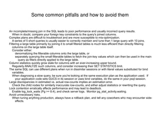
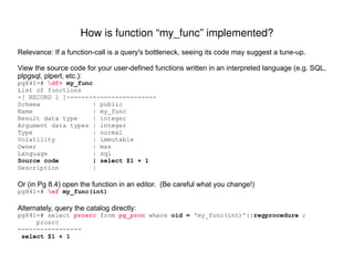
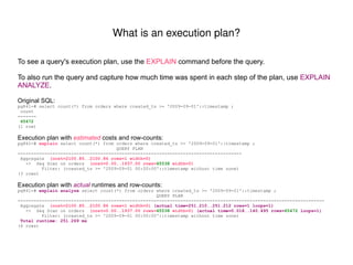
29. Stale or missing statistics: When was my table last analyzed? Review the last time when each table was analyzed (either manually or by autovacuum). Use your knowledge of how and when your data changes to decide if the statistics are likely to be out of date. pg841=# select pg841-# schemaname, pg841-# relname, pg841-# last_analyze as last_manual, pg841-# last_autoanalyze as last_auto, pg841-# greatest (last_analyze, last_autoanalyze) pg841-# from pg841-# pg_stat_user_tables pg841-# where pg841-# relname = 'my_tab' pg841-# ; -[ RECORD 1 ]------------------------------ schemaname | public relname | my_tab last_manual | 2009-10-03 18:45:57.627593-07 last_auto | 2009-10-03 23:08:32.914092-07 greatest | 2009-10-03 23:08:32.914092-07

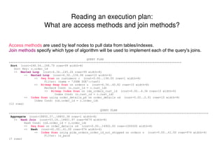
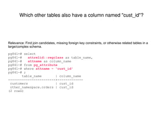
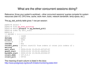
30. Stale or missing statistics: How many rows does the optimizer think my table has? How are my columns' values distributed? Many bad plans are due to poor cardinality estimates for one or more nodes. Sometimes this is due to stale or missing statistics. For example, if a column was added or a significant percentage of rows were inserted, deleted, or modified, then the optimizer statistics should be refreshed. You can view the table-level optimizer statistics in pg_class: pg841=# select reltuples , relpages from pg_class where relname = 'my_tab' ; reltuples | relpages -----------+---------- 1000 | 5 (1 row) And the more detailed column-level optimizer statistics are shown in pg_stats: pg841=# select * from pg_stats where tablename = 'my_tab' and attname = 'bar' ; -[ RECORD 1 ]-----+--------------------------- schemaname | public tablename | my_tab attname | bar null_frac | 0 avg_width | 4 n_distinct | 13 most_common_vals | {1,2} most_common_freqs | {0.707,0.207} histogram_bounds | {0,3,4,5,6,7,8,9,10,11,12} correlation | 0.876659

31. A new index is usually helpful if it greatly reduces the number of rows the query must visit. This table has an index for all possible combinations of its columns. pg841=# \d my_tab Table "public.my_tab" Column | Type | Modifiers --------+---------+----------- foo | integer | bar | integer | Indexes: "idx_my_tab_bar" btree (bar) "idx_my_tab_bar_foo" btree (bar, foo) "idx_my_tab_foo" btree (foo) "idx_my_tab_foo_bar" btree (foo, bar) At least 1 is unnecessary, and up to 2 could be dropped without forcing any query to use a Seq Scan. pg841=# explain select * from my_tab where foo = 10 and bar = 10 ; QUERY PLAN --------------------------------------------------------------------------------- Index Scan using idx_my_tab_bar_foo on my_tab (cost=0.00..8.27 rows=1 width=8) Index Cond: ((bar = 10) AND (foo = 10)) (2 rows) pg841=# drop index idx_my_tab_bar_foo ; DROP INDEX pg841=# drop index idx_my_tab_foo_bar ; DROP INDEX pg841=# explain select * from my_tab where foo = 10 and bar = 10 ; QUERY PLAN ----------------------------------------------------------------------------- Index Scan using idx_my_tab_foo on my_tab (cost=0.00..8.27 rows=1 width=8) Index Cond: (foo = 10) Filter: (bar = 10) (3 rows) When will adding a new index improve query performance?