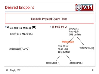
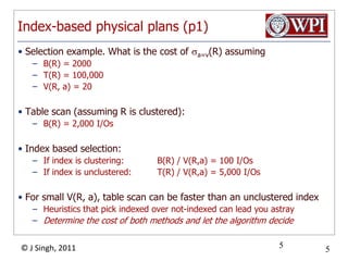
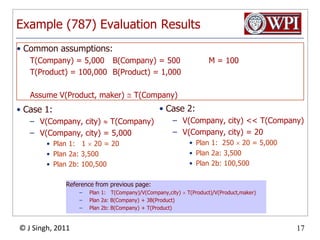
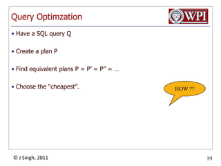
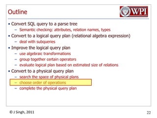
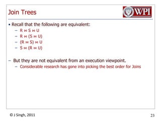
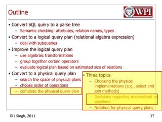
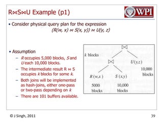
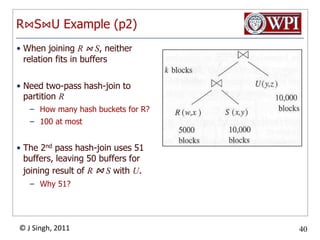
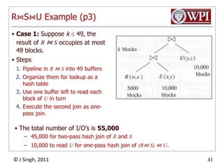
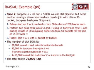
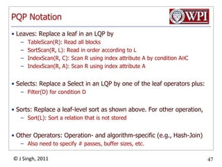
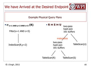
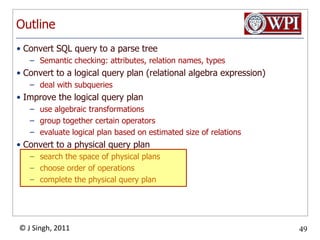
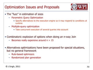
CS 542 Database Management SystemsQuery OptimizationJ Singh March 28, 2011
OutlineConvert SQL query to a parse treeSemantic checking: attributes, relation names, typesConvert to a logical query plan (relational algebra expression)deal with subqueriesImprove the logical query planuse algebraic transformationsgroup together certain operatorsevaluate logical plan based on estimated size of relations Convert to a physical query plansearch the space of physical plans choose order of operationscomplete the physical query plan
Desired Endpoint x=1 AND y=2 AND z<5 (R)R ⋈ S ⋈ UExample Physical Query Planstwo-passhash-join101 buffersFilter(x=1 AND z<5)materializeIndexScan(R,y=2)two-passhash-join101 buffersTableScan(U)TableScan(R)TableScan(S)
Physical Plan SelectionThe particular operation being performedSize of intermediate results, as derived last week (sec 16.4 of book)Physical Operator Implementation used, e.g., one- or two-passOperation ordering, esp. Join orderingOperation output: materialized or pipelined.Governed by disk I/O, which in turn is governed by
Index-based physical plans (p1)Selection example. What is the cost of a=v(R) assumingB(R) = 2000T(R) = 100,000V(R, a) = 20Table scan (assuming R is clustered):B(R) = 2,000 I/OsIndex based selection:If index is clustering: 	B(R) / V(R,a) = 100 I/OsIf index is unclustered: 	T(R) / V(R,a) = 5,000 I/OsFor small V(R, a), table scan can be faster than an unclustered indexHeuristics that pick indexed over not-indexed can lead you astrayDetermine the cost of both methods and let the algorithm decide5
Index-based physical plans (p2)Example: Join if S has an index on the join attributeFor each tuplein R, fetch corresponding tuple(s) from SAssume R is clustered. Cost:If index on S is clustering:	B(R) + T(R) B(S) / V(S,a)If index on S is unclustered:	B(R) + T(R) T(S) / V(S,a)Another case: when R is output of another Iterator. Cost:B(R) is accounted for in the iteratorIf index on S is clustering:	T(R) B(S) / V(S,a)If index on S is unclustered:	T(R) T(S) / V(S,a)If S is not indexed but fits in memory: B(S)A number of other cases
Index-based physical plans (p3)Index Based Join ifboth R and S have a sorted index (B+ tree) on the join attributeThen perform a merge join called zig-zag joinCost: B(R) + B(S)
Grand Summary of Physical Plans (p1)Scans and SelectsIndex: N = None, C = Clustering, NC = Non-clustered
Grand Summary of Physical Plans (p2)JoinsIndex: N = None, C = Clustering, NC = Non-clusteredRelation fits in memory: F = Yes, NF = No
Physical plans at non-leaf Operators (p1)What if the input of the operator is from another operator?For Select, cost= 0.Cost of pipelining is assumed to be zeroThe number of tuples emitted is reducedFor Join, when R is from an operator and S from a table:B(R) is accounted for in the iteratorIf index on S is clustering:	T(R) B(S) / V(S,a)If index on S is unclustered:	T(R) T(S) / V(S,a)If S is not indexed but fits in memory: B(S)If S is not indexed and doesn’t fit: k*B(S) for k chunksIf S is not indexed and doesn’t fit: 3*B(S) for sort- or hash-join
Physical plans at non-leaf Operators (p2)For Join, when R and S are both from operators, cost depends on whether the result are sorted by the Join attribute(s)If yes, we use the zig-zag algorithm and the cost is zero. Why?If either relation will fit in memory, the cost is zero. Why?At most, the cost is 2*(B(R) + B(S)). Why?
Example (787)Product(pname, maker), Company(cname, city)Select Product.pnameFrom  Product, CompanyWhere Product.maker=Company.cname    and  Company.city = “Seattle”How do we execute this query ?
Example (787)Product(pname, maker), Company(cname, city)Select Product.pnameFrom  Product, CompanyWhere Product.maker=Company.cname    and  Company.city = “Seattle”Logical PlanClustering Indices:Product.pnameCompany.cnameUnclustered Indices:Product.makerCompany.citymaker=cnamescity=“Seattle”Product(pname,maker)Company(cname,city)
Example (787) Physical PlansPhysical Plan 1Physical Plans 2a and 2bMerge-joinIndex-basedjoinIndex-basedselectionmaker=cnamescity=“Seattle”cname=makerscity=“Seattle”Product(pname,maker)Company(cname,city)Product(pname,maker)Company(cname,city)Index-scanScan and sort (2a)index scan (2b)
Evaluate (787) Physical PlansPhysical Plan 1Tuples:T(city='Seattle'(Company)) = T(Company) / V(Company, City)Cost:T(city='Seattle'(Company))  * T(Product) / V(Product, maker)or, simplifying,T(Company) / V(Company, City) * T(Product) / V(Product, maker)Total Cost:2a: 3B(Product) + B(Company)2b: T(Product) + B(Company)Merge-joinmaker=cnamescity=“Seattle”Product(pname,maker)Company(cname,city)Index-scanScan and sort (2a)index scan (2b)
Final EvaluationPlan Costs:Plan 1: T(Company) / V(Company, city)  T(Product)/V(Product, maker)Plan 2a: B(Company) + 3B(Product)Plan 2b: B(Company) + T(Product)Which is better?It depends on the data
Example (787) Evaluation ResultsCommon assumptions:T(Company) = 5,000	B(Company) = 500	M = 100T(Product) = 100,000	B(Product) = 1,000Assume V(Product, maker)  T(Company)Case 2: V(Company, city) << T(Company)V(Company, city) = 20Plan 1:  250  20 = 5,000Plan 2a: 3,500Plan 2b: 100,500Case 1: V(Company, city)  T(Company)V(Company, city) = 5,000 Plan 1:   1  20 = 20Plan 2a: 3,500Plan 2b: 100,500Reference from previous page:Plan 1:   T(Company)/V(Company,city)  T(Product)/V(Product,maker)
Plan 2a: B(Company) + 3B(Product)
Plan 2b: B(Company) + T(Product)LessonsNeed to consider several physical planseven for one, simple logical planNo magic “best” plan: depends on the dataIn order to make the right choiceneed to have statistics over the datathe B’s, the T’s, the V’s
Query OptimzationHave a SQL query QCreate a plan PFind equivalent plans P = P’ = P’’ = … Choose the “cheapest”.  HOW ??
Logical Query PlanSELECT  P.buyerFROM Purchase P, Person QWHERE P.buyer=Q.name ANDQ.city=‘seattle’ AND Q.phone > ‘5430000’ PlanbuyerCity=‘seattle’  phone>’5430000’Buyer=nameIn class:find a “better” plan P’PersonPurchase
CS 542 Database Management SystemsQuery Optimization – Choosing the Order of OperationsJ Singh March 28, 2011
OutlineConvert SQL query to a parse treeSemantic checking: attributes, relation names, typesConvert to a logical query plan (relational algebra expression)deal with subqueriesImprove the logical query planuse algebraic transformationsgroup together certain operatorsevaluate logical plan based on estimated size of relations Convert to a physical query plansearch the space of physical plans choose order of operationscomplete the physical query plan
Join TreesRecall that the following are equivalent:R ⋈ S ⋈ U
R ⋈ (S ⋈ U)
(R ⋈ S) ⋈ U
S ⋈ (R ⋈ U)
But they are not equivalent from an execution viewpoint.Considerable research has gone into picking the best order for Joins
Join TreesR1 ⋈R2 ⋈ …⋈RnJoin tree:DefinitionsA plan = a join treeA partial plan = a subtree of a join treeR3R1R2R424
Left & Right Join ArgumentsThe argument relations in joins determine the cost of the joinIn Physical Query Plans, the left argument of the join is Called the build relationAssumed to be smallerStored in main-memory
Left & Right Join ArgumentsThe right argument of the join isCalled the probe relation Read a block at a timeIts tuples are matched with those of build relationThe join algorithms which distinguish between the arguments are:One-pass joinNested-loop joinIndex join
Types of Join TreesRight deepLeft deep:BushyR3R4R1R2R5R3R2R4R5R2R4R3R1Many different orders, very important to pick the right oneR5R1
Optimization AlgorithmsHeuristic basedCost basedDynamic programming: System RRule-based optimizations: DB2, SQL-Server
Dynamic ProgrammingGiven: a query  R1 ⋈R2 ⋈… ⋈RnAssume we have a function cost() that gives us the cost of a join treeFind the best join tree for the query
Dynamic ProgrammingProblem StatementGiven: a query  R1 ⋈ R2 ⋈… ⋈RnAssume we have a function cost() that gives us the cost of a join treeFind the best join tree for the queryIdea: for each subset of {R1, …, Rn}, compute the best plan for that subsetAlgorithm: In increasing order of set cardinality, compute the cost forStep 1: for {R1}, {R2}, …, {Rn}Step 2: for {R1,R2}, {R1,R3}, …, {Rn-1, Rn}…Step n: for {R1, …, Rn}It is a bottom-up strategySkipping further details of the algorithmRead from book if interestedWill not be on the exam
Dynamic Programming AlgorithmWhen computing R1 ⋈ R2 ⋈ … ⋈ Rn,Best Plan (R1 ⋈ R2 ⋈ … ⋈ Rn) = min cost plan ofBest Plan (R2 ⋈ R3 ⋈ … ⋈ Rn) ⋈ R1
Best Plan (R1 ⋈ R3 ⋈ … ⋈ Rn) ⋈ R2
…
Best Plan (R1 ⋈ R2 ⋈ … ⋈ Rn-1) ⋈ RnReducing the Search Space Left-deep trees vsBushy treesCombinatoric explosion of the number of possible treesComputing the cost of all possible trees is not feasibleFor a 6-way Join, we can haveMore than 30,000 bushy trees6!, or 720 left-deep treesLeft-deep trees leave their result in memory, making it possible to pipeline efficientlyTrees without Cartesian productExample:  R(A,B) ⋈S(B,C) ⋈ T(C,D)Plan: (R(A,B) ⋈T(C,D)) ⋈S(B,C) has a Cartesian productMost query optimizers will not consider it
OutlineConvert SQL query to a parse treeSemantic checking: attributes, relation names, typesConvert to a logical query plan (relational algebra expression)deal with subqueriesImprove the logical query planuse algebraic transformationsgroup together certain operatorsevaluate logical plan based on estimated size of relations Convert to a physical query plansearch the space of physical plans choose order of operationscomplete the physical query planThree topicsChoosing the physical implementations (e.g., select and join methods)Decisions regarding materialized vs pipelinedNotation for physical query plans
Choosing a Selection MethodAlgorithm for each selection operator1. Can we use an created index on an attribute?If yes, index-scan. (Otherwise table-scan)2. After retrieving all condition-satisfied tuples in (1), filter them with the remaining selection conditionsIn other words,When computing c1  c2  …  cn(R), we index-scan on ci, then filter the result on all other ci, where j  i.The next 2 pages show an example where we examine several options and pick the best one
Selection Method Example (p1)Selection: x=1  y=2  z < 5 (R)Where parameters of R are:	T(R) = 5,000		B(R) = 200	V(R, x) = 100		V(R, y) = 500Relation R is clusteredx and y have non-clustering indicesz is a clustering index
Selection Method Example (p2)Selection options:Table-scan  filter x, y, z. Cost isB(R) =  200since R is clustered.Use index on x =1  filter on y, z.  Cost is 50 sinceT(R) / V(R, x) is (5000/100) = 50 tuples, x is not clustering.Use index on y =2  filter on x, z.  Cost is 10 sinceT(R) / V(R, y) is (5000/500) = 10 tuples, y is not clustering.Index-scan on clustering index w/ z < 5 filter x ,y.  Cost is about B(R)/3 = 67Therefore:First retrieve all tuples with y = 2 (option 3)Then filter for x and z
OutlineConvert SQL query to a parse treeSemantic checking: attributes, relation names, typesConvert to a logical query plan (relational algebra expression)deal with subqueriesImprove the logical query planuse algebraic transformationsgroup together certain operatorsevaluate logical plan based on estimated size of relations Convert to a physical query plansearch the space of physical plans choose order of operationscomplete the physical query planThree topicsChoosing the physical implementations (e.g., select and join methods)Decisions regarding materialized vs pipelinedNotation for physical query plans
Pipelining Versus MaterializationMaterializationstore (intermediate) result of each operations on disk PipeliningInterleave the execution of several operations, the tuples produced by one operation are passed directly to the operations that used itstore (intermediate) result of each operations on buffer, which is implemented on main memoryPrefer Pipelining where possibleSometimes not possible, as the following example showsNext few pages, a fully worked-out example
R⋈S⋈U Example (p1)Consider physical query plan for the expression(R(w, x) ⋈ S(x, y)) ⋈ U(y, z)AssumptionR occupies 5,000 blocks, S and U each 10,000 blocks.The intermediate result R ⋈ S occupies k blocks for some k.Both joins will be implemented as hash-joins, either one-pass or two-pass depending on kThere are 101 buffers available.
R⋈S⋈U Example (p2)When joining R ⋈ S, neither relation fits in buffersNeed two-pass hash-join to partition RHow many hash buckets for R?100 at mostThe 2nd pass hash-join uses 51 buffers, leaving 50 buffers for joining result of R ⋈ S with U.Why 51?
R⋈S⋈U Example (p3)Case 1: Suppose k 49, the result of R ⋈ S occupies at most 49 blocks. Steps Pipeline in R ⋈ S into 49 buffersOrganize them for lookup as a hash tableUse one buffer left to read each block of U in turnExecute the second join as one-pass join.The total number of I/O’s is 55,00045,000 for two-pass hash join of R and S10,000 to read U for one-pass hash join of (R⋈ S) ⋈U.
R⋈S⋈U Example (p4)Case 2: suppose k > 49 but < 5,000, we can still pipeline, but need another strategy where intermediate results join with U in a 50-bucket, two-pass hash-join. Steps are:Before start on R ⋈ S, we hash U into 50 buckets of 200 blocks each.Perform two-pass hash join of R and U using 51 buffers as case 1, and placing results in 50 remaining buffers to form 50 buckets for the join of  R ⋈ S with U.Finally, join R ⋈ S with U bucket by bucket. The number of disk I/O’s is:20,000 to read U and write its tuples into buckets45,000 for two-pass hash-join R ⋈ Sk to write out the buckets of R ⋈ Sk+10,000 to read the buckets of R ⋈ S and U in the final joinThe total cost is 75,000+2k.
R⋈S⋈U Example (p5)Case 3: k > 5,000, we cannot perform two-pass join in 50 buffers available if result of R ⋈ S is pipelined. We are forced to materialize the relation R ⋈ S. The number of disk I/O’s is:45,000 for two-pass hash-join R and Sk to store R ⋈ S on disk30,000 + 3k for two-pass join of U in R ⋈ SThe total cost is 75,000+4k.
R⋈S⋈U Example (p6)In summary, costs of physical plan as function of R ⋈ S size.Pause and ReflectIt’s all about the expected size of the intermediate result R ⋈ SWhat would have happened if We guessed 45 but had 55? 		Guessed 55 but only had 45?Guessed 4,500 but had 5,500?	Guessed 5,500 but only had 4,500?
OutlineConvert SQL query to a parse treeSemantic checking: attributes, relation names, typesConvert to a logical query plan (relational algebra expression)deal with subqueriesImprove the logical query planuse algebraic transformationsgroup together certain operatorsevaluate logical plan based on estimated size of relations Convert to a physical query plansearch the space of physical plans choose order of operationscomplete the physical query planThree topicsChoosing the physical implementations (e.g., select and join methods)Decisions regarding materialized vs pipelinedNotation for physical query plans
Notation for Physical Query PlansSeveral types of operators: Operators for leaves(Physical) operators for Selection(Physical) Sorts OperatorsOther Relational-Algebra OperationsIn practice, each DBMS uses its own internal notation for physical query plans
PQP NotationLeaves:Replace a leaf in an LQP byTableScan(R): Read all blocksSortScan(R, L): Read in order according to LIndexScan(R, C): Scan R using index attribute A by condition ACIndexScan(R, A): Scan R using index attribute ASelects: Replace a Select in an LQP by one of the leaf operators plus:Filter(D) for condition DSorts: Replace a leaf-level sort as shown above. For other operation,Sort(L): Sort a relation that is not storedOther Operators: Operation- and algorithm-specific (e.g., Hash-Join)Also need to specify # passes, buffer sizes, etc.
We have Arrived at the Desired Endpoint x=1 AND y=2 AND z<5 (R)R ⋈ S ⋈ UExample Physical Query Planstwo-passhash-join101 buffersFilter(x=1 AND z<5)materializeIndexScan(R,y=2)two-passhash-join101 buffersTableScan(U)TableScan(R)TableScan(S)
OutlineConvert SQL query to a parse treeSemantic checking: attributes, relation names, typesConvert to a logical query plan (relational algebra expression)deal with subqueriesImprove the logical query planuse algebraic transformationsgroup together certain operatorsevaluate logical plan based on estimated size of relations Convert to a physical query plansearch the space of physical plans choose order of operationscomplete the physical query plan
Optimization Issues and ProposalsThe “fuzz” in estimation of sizesParametric Query OptimizationSpecify alternatives to the execution engine so it may respond to conditions at runtimeMultiple-query optimizationTake concurrent execution of several queries into accountCombinatoric explosion of options when doing an n-way JoinBecomes really expensive around n > 15Alternatives optimizations have been proposed for special situations, but no general frameworkRule-based optimizersRandomized plan generation
CS 542 Database Management SystemsDistributed Query ExecutionSource: Carsten Binnig, Univ of Zurich, 2006J Singh March 28, 2011
MotivationAlgorithms based on Semi-Joins have been proposed as techniques for query optimizationThey shine in Distributed and Parallel DatabasesGood opportunity to explore them in that contextSemi-join by example:Semi-join formal definition:
Distributed / Parallel Join ProcessingScenario:How to compute A ⋈B?Table A resides on Node 1Table B resides on Node 2Node 1Node 2Table ATable B
Naïve approach (1)Idea: Use standard join and fetch table page-wise from remote node if necessary (send- and receive-operators)Example:Join is executed on node 2 using a Nested-Loop-JoinOuter loop: Request page of table A from node 1 (remote)Inner loop: For each page iterate over table B and produce output=> Random access of pages on node 1 (due to network delay)Node 1Node 2RequestTable APage A1Table BSend
Naïve approach (2)Idea: Ship one table completely to the other nodeExample:Ship complete table A from node 1 to node 2Join table A and B locally on node 2Avoid random page access on node 1Node 1Node 2Table ATable ATable BShip
Naïve Approach: ImplicationsProblems:High cost for shipping dataNetwork cost roughly the same as I/O cost for a hard disk (or even worse because of unpredictability of network delay)Shipping A roughly equivalent to a full table scan(Trivial) Optimizations:Ship always smaller table to the other sideIf query contains a selection, apply selection before sending ANote: bigger table may become the smaller table (after selection)
Semi-join Approach (p1)Idea: Before shipping a table, reduce to data that is shipped to those tuples that are only relevant for joinExample: Join on A.id=B.id and table A should be shipped to node 2Node 1Node 2Table ATable B
Semi-join Approach (p2)(1) Compute projection B.id of table B on node 2(2) Ship column B.id to node 1Node 1Node 2Table ATable BShip
Semi-join Approach (p3)(3) Execute semi-join of B.id and table A on A.id=B.id (to select only relevant tuples of table A => table A’)(4) Send result of semi-join (table A’) to node 2Node 1Node 2Table ATable BTable A’Ship

CS 542 -- Query Optimization

  • 1.
    CS 542 DatabaseManagement SystemsQuery OptimizationJ Singh March 28, 2011
  • 2.
    OutlineConvert SQL queryto a parse treeSemantic checking: attributes, relation names, typesConvert to a logical query plan (relational algebra expression)deal with subqueriesImprove the logical query planuse algebraic transformationsgroup together certain operatorsevaluate logical plan based on estimated size of relations Convert to a physical query plansearch the space of physical plans choose order of operationscomplete the physical query plan
  • 3.
    Desired Endpoint x=1AND y=2 AND z<5 (R)R ⋈ S ⋈ UExample Physical Query Planstwo-passhash-join101 buffersFilter(x=1 AND z<5)materializeIndexScan(R,y=2)two-passhash-join101 buffersTableScan(U)TableScan(R)TableScan(S)
  • 4.
    Physical Plan SelectionTheparticular operation being performedSize of intermediate results, as derived last week (sec 16.4 of book)Physical Operator Implementation used, e.g., one- or two-passOperation ordering, esp. Join orderingOperation output: materialized or pipelined.Governed by disk I/O, which in turn is governed by
  • 5.
    Index-based physical plans(p1)Selection example. What is the cost of a=v(R) assumingB(R) = 2000T(R) = 100,000V(R, a) = 20Table scan (assuming R is clustered):B(R) = 2,000 I/OsIndex based selection:If index is clustering: B(R) / V(R,a) = 100 I/OsIf index is unclustered: T(R) / V(R,a) = 5,000 I/OsFor small V(R, a), table scan can be faster than an unclustered indexHeuristics that pick indexed over not-indexed can lead you astrayDetermine the cost of both methods and let the algorithm decide5
  • 6.
    Index-based physical plans(p2)Example: Join if S has an index on the join attributeFor each tuplein R, fetch corresponding tuple(s) from SAssume R is clustered. Cost:If index on S is clustering: B(R) + T(R) B(S) / V(S,a)If index on S is unclustered: B(R) + T(R) T(S) / V(S,a)Another case: when R is output of another Iterator. Cost:B(R) is accounted for in the iteratorIf index on S is clustering: T(R) B(S) / V(S,a)If index on S is unclustered: T(R) T(S) / V(S,a)If S is not indexed but fits in memory: B(S)A number of other cases
  • 7.
    Index-based physical plans(p3)Index Based Join ifboth R and S have a sorted index (B+ tree) on the join attributeThen perform a merge join called zig-zag joinCost: B(R) + B(S)
  • 8.
    Grand Summary ofPhysical Plans (p1)Scans and SelectsIndex: N = None, C = Clustering, NC = Non-clustered
  • 9.
    Grand Summary ofPhysical Plans (p2)JoinsIndex: N = None, C = Clustering, NC = Non-clusteredRelation fits in memory: F = Yes, NF = No
  • 10.
    Physical plans atnon-leaf Operators (p1)What if the input of the operator is from another operator?For Select, cost= 0.Cost of pipelining is assumed to be zeroThe number of tuples emitted is reducedFor Join, when R is from an operator and S from a table:B(R) is accounted for in the iteratorIf index on S is clustering: T(R) B(S) / V(S,a)If index on S is unclustered: T(R) T(S) / V(S,a)If S is not indexed but fits in memory: B(S)If S is not indexed and doesn’t fit: k*B(S) for k chunksIf S is not indexed and doesn’t fit: 3*B(S) for sort- or hash-join
  • 11.
    Physical plans atnon-leaf Operators (p2)For Join, when R and S are both from operators, cost depends on whether the result are sorted by the Join attribute(s)If yes, we use the zig-zag algorithm and the cost is zero. Why?If either relation will fit in memory, the cost is zero. Why?At most, the cost is 2*(B(R) + B(S)). Why?
  • 12.
    Example (787)Product(pname, maker),Company(cname, city)Select Product.pnameFrom Product, CompanyWhere Product.maker=Company.cname and Company.city = “Seattle”How do we execute this query ?
  • 13.
    Example (787)Product(pname, maker),Company(cname, city)Select Product.pnameFrom Product, CompanyWhere Product.maker=Company.cname and Company.city = “Seattle”Logical PlanClustering Indices:Product.pnameCompany.cnameUnclustered Indices:Product.makerCompany.citymaker=cnamescity=“Seattle”Product(pname,maker)Company(cname,city)
  • 14.
    Example (787) PhysicalPlansPhysical Plan 1Physical Plans 2a and 2bMerge-joinIndex-basedjoinIndex-basedselectionmaker=cnamescity=“Seattle”cname=makerscity=“Seattle”Product(pname,maker)Company(cname,city)Product(pname,maker)Company(cname,city)Index-scanScan and sort (2a)index scan (2b)
  • 15.
    Evaluate (787) PhysicalPlansPhysical Plan 1Tuples:T(city='Seattle'(Company)) = T(Company) / V(Company, City)Cost:T(city='Seattle'(Company)) * T(Product) / V(Product, maker)or, simplifying,T(Company) / V(Company, City) * T(Product) / V(Product, maker)Total Cost:2a: 3B(Product) + B(Company)2b: T(Product) + B(Company)Merge-joinmaker=cnamescity=“Seattle”Product(pname,maker)Company(cname,city)Index-scanScan and sort (2a)index scan (2b)
  • 16.
    Final EvaluationPlan Costs:Plan1: T(Company) / V(Company, city)  T(Product)/V(Product, maker)Plan 2a: B(Company) + 3B(Product)Plan 2b: B(Company) + T(Product)Which is better?It depends on the data
  • 17.
    Example (787) EvaluationResultsCommon assumptions:T(Company) = 5,000 B(Company) = 500 M = 100T(Product) = 100,000 B(Product) = 1,000Assume V(Product, maker)  T(Company)Case 2: V(Company, city) << T(Company)V(Company, city) = 20Plan 1: 250  20 = 5,000Plan 2a: 3,500Plan 2b: 100,500Case 1: V(Company, city)  T(Company)V(Company, city) = 5,000 Plan 1: 1  20 = 20Plan 2a: 3,500Plan 2b: 100,500Reference from previous page:Plan 1: T(Company)/V(Company,city)  T(Product)/V(Product,maker)
  • 18.
    Plan 2a: B(Company)+ 3B(Product)
  • 19.
    Plan 2b: B(Company)+ T(Product)LessonsNeed to consider several physical planseven for one, simple logical planNo magic “best” plan: depends on the dataIn order to make the right choiceneed to have statistics over the datathe B’s, the T’s, the V’s
  • 20.
    Query OptimzationHave aSQL query QCreate a plan PFind equivalent plans P = P’ = P’’ = … Choose the “cheapest”. HOW ??
  • 21.
    Logical Query PlanSELECT P.buyerFROM Purchase P, Person QWHERE P.buyer=Q.name ANDQ.city=‘seattle’ AND Q.phone > ‘5430000’ PlanbuyerCity=‘seattle’ phone>’5430000’Buyer=nameIn class:find a “better” plan P’PersonPurchase
  • 22.
    CS 542 DatabaseManagement SystemsQuery Optimization – Choosing the Order of OperationsJ Singh March 28, 2011
  • 23.
    OutlineConvert SQL queryto a parse treeSemantic checking: attributes, relation names, typesConvert to a logical query plan (relational algebra expression)deal with subqueriesImprove the logical query planuse algebraic transformationsgroup together certain operatorsevaluate logical plan based on estimated size of relations Convert to a physical query plansearch the space of physical plans choose order of operationscomplete the physical query plan
  • 24.
    Join TreesRecall thatthe following are equivalent:R ⋈ S ⋈ U
  • 25.
    R ⋈ (S⋈ U)
  • 26.
  • 27.
    S ⋈ (R⋈ U)
  • 28.
    But they arenot equivalent from an execution viewpoint.Considerable research has gone into picking the best order for Joins
  • 29.
    Join TreesR1 ⋈R2⋈ …⋈RnJoin tree:DefinitionsA plan = a join treeA partial plan = a subtree of a join treeR3R1R2R424
  • 30.
    Left & RightJoin ArgumentsThe argument relations in joins determine the cost of the joinIn Physical Query Plans, the left argument of the join is Called the build relationAssumed to be smallerStored in main-memory
  • 31.
    Left & RightJoin ArgumentsThe right argument of the join isCalled the probe relation Read a block at a timeIts tuples are matched with those of build relationThe join algorithms which distinguish between the arguments are:One-pass joinNested-loop joinIndex join
  • 32.
    Types of JoinTreesRight deepLeft deep:BushyR3R4R1R2R5R3R2R4R5R2R4R3R1Many different orders, very important to pick the right oneR5R1
  • 33.
    Optimization AlgorithmsHeuristic basedCostbasedDynamic programming: System RRule-based optimizations: DB2, SQL-Server
  • 34.
    Dynamic ProgrammingGiven: aquery R1 ⋈R2 ⋈… ⋈RnAssume we have a function cost() that gives us the cost of a join treeFind the best join tree for the query
  • 35.
    Dynamic ProgrammingProblem StatementGiven:a query R1 ⋈ R2 ⋈… ⋈RnAssume we have a function cost() that gives us the cost of a join treeFind the best join tree for the queryIdea: for each subset of {R1, …, Rn}, compute the best plan for that subsetAlgorithm: In increasing order of set cardinality, compute the cost forStep 1: for {R1}, {R2}, …, {Rn}Step 2: for {R1,R2}, {R1,R3}, …, {Rn-1, Rn}…Step n: for {R1, …, Rn}It is a bottom-up strategySkipping further details of the algorithmRead from book if interestedWill not be on the exam
  • 36.
    Dynamic Programming AlgorithmWhencomputing R1 ⋈ R2 ⋈ … ⋈ Rn,Best Plan (R1 ⋈ R2 ⋈ … ⋈ Rn) = min cost plan ofBest Plan (R2 ⋈ R3 ⋈ … ⋈ Rn) ⋈ R1
  • 37.
    Best Plan (R1⋈ R3 ⋈ … ⋈ Rn) ⋈ R2
  • 38.
  • 39.
    Best Plan (R1⋈ R2 ⋈ … ⋈ Rn-1) ⋈ RnReducing the Search Space Left-deep trees vsBushy treesCombinatoric explosion of the number of possible treesComputing the cost of all possible trees is not feasibleFor a 6-way Join, we can haveMore than 30,000 bushy trees6!, or 720 left-deep treesLeft-deep trees leave their result in memory, making it possible to pipeline efficientlyTrees without Cartesian productExample: R(A,B) ⋈S(B,C) ⋈ T(C,D)Plan: (R(A,B) ⋈T(C,D)) ⋈S(B,C) has a Cartesian productMost query optimizers will not consider it
  • 40.
    OutlineConvert SQL queryto a parse treeSemantic checking: attributes, relation names, typesConvert to a logical query plan (relational algebra expression)deal with subqueriesImprove the logical query planuse algebraic transformationsgroup together certain operatorsevaluate logical plan based on estimated size of relations Convert to a physical query plansearch the space of physical plans choose order of operationscomplete the physical query planThree topicsChoosing the physical implementations (e.g., select and join methods)Decisions regarding materialized vs pipelinedNotation for physical query plans
  • 41.
    Choosing a SelectionMethodAlgorithm for each selection operator1. Can we use an created index on an attribute?If yes, index-scan. (Otherwise table-scan)2. After retrieving all condition-satisfied tuples in (1), filter them with the remaining selection conditionsIn other words,When computing c1  c2  …  cn(R), we index-scan on ci, then filter the result on all other ci, where j  i.The next 2 pages show an example where we examine several options and pick the best one
  • 42.
    Selection Method Example(p1)Selection: x=1  y=2  z < 5 (R)Where parameters of R are: T(R) = 5,000 B(R) = 200 V(R, x) = 100 V(R, y) = 500Relation R is clusteredx and y have non-clustering indicesz is a clustering index
  • 43.
    Selection Method Example(p2)Selection options:Table-scan  filter x, y, z. Cost isB(R) = 200since R is clustered.Use index on x =1  filter on y, z. Cost is 50 sinceT(R) / V(R, x) is (5000/100) = 50 tuples, x is not clustering.Use index on y =2  filter on x, z. Cost is 10 sinceT(R) / V(R, y) is (5000/500) = 10 tuples, y is not clustering.Index-scan on clustering index w/ z < 5 filter x ,y. Cost is about B(R)/3 = 67Therefore:First retrieve all tuples with y = 2 (option 3)Then filter for x and z
  • 44.
    OutlineConvert SQL queryto a parse treeSemantic checking: attributes, relation names, typesConvert to a logical query plan (relational algebra expression)deal with subqueriesImprove the logical query planuse algebraic transformationsgroup together certain operatorsevaluate logical plan based on estimated size of relations Convert to a physical query plansearch the space of physical plans choose order of operationscomplete the physical query planThree topicsChoosing the physical implementations (e.g., select and join methods)Decisions regarding materialized vs pipelinedNotation for physical query plans
  • 45.
    Pipelining Versus MaterializationMaterializationstore(intermediate) result of each operations on disk PipeliningInterleave the execution of several operations, the tuples produced by one operation are passed directly to the operations that used itstore (intermediate) result of each operations on buffer, which is implemented on main memoryPrefer Pipelining where possibleSometimes not possible, as the following example showsNext few pages, a fully worked-out example
  • 46.
    R⋈S⋈U Example (p1)Considerphysical query plan for the expression(R(w, x) ⋈ S(x, y)) ⋈ U(y, z)AssumptionR occupies 5,000 blocks, S and U each 10,000 blocks.The intermediate result R ⋈ S occupies k blocks for some k.Both joins will be implemented as hash-joins, either one-pass or two-pass depending on kThere are 101 buffers available.
  • 47.
    R⋈S⋈U Example (p2)Whenjoining R ⋈ S, neither relation fits in buffersNeed two-pass hash-join to partition RHow many hash buckets for R?100 at mostThe 2nd pass hash-join uses 51 buffers, leaving 50 buffers for joining result of R ⋈ S with U.Why 51?
  • 48.
    R⋈S⋈U Example (p3)Case1: Suppose k 49, the result of R ⋈ S occupies at most 49 blocks. Steps Pipeline in R ⋈ S into 49 buffersOrganize them for lookup as a hash tableUse one buffer left to read each block of U in turnExecute the second join as one-pass join.The total number of I/O’s is 55,00045,000 for two-pass hash join of R and S10,000 to read U for one-pass hash join of (R⋈ S) ⋈U.
  • 49.
    R⋈S⋈U Example (p4)Case2: suppose k > 49 but < 5,000, we can still pipeline, but need another strategy where intermediate results join with U in a 50-bucket, two-pass hash-join. Steps are:Before start on R ⋈ S, we hash U into 50 buckets of 200 blocks each.Perform two-pass hash join of R and U using 51 buffers as case 1, and placing results in 50 remaining buffers to form 50 buckets for the join of R ⋈ S with U.Finally, join R ⋈ S with U bucket by bucket. The number of disk I/O’s is:20,000 to read U and write its tuples into buckets45,000 for two-pass hash-join R ⋈ Sk to write out the buckets of R ⋈ Sk+10,000 to read the buckets of R ⋈ S and U in the final joinThe total cost is 75,000+2k.
  • 50.
    R⋈S⋈U Example (p5)Case3: k > 5,000, we cannot perform two-pass join in 50 buffers available if result of R ⋈ S is pipelined. We are forced to materialize the relation R ⋈ S. The number of disk I/O’s is:45,000 for two-pass hash-join R and Sk to store R ⋈ S on disk30,000 + 3k for two-pass join of U in R ⋈ SThe total cost is 75,000+4k.
  • 51.
    R⋈S⋈U Example (p6)Insummary, costs of physical plan as function of R ⋈ S size.Pause and ReflectIt’s all about the expected size of the intermediate result R ⋈ SWhat would have happened if We guessed 45 but had 55? Guessed 55 but only had 45?Guessed 4,500 but had 5,500? Guessed 5,500 but only had 4,500?
  • 52.
    OutlineConvert SQL queryto a parse treeSemantic checking: attributes, relation names, typesConvert to a logical query plan (relational algebra expression)deal with subqueriesImprove the logical query planuse algebraic transformationsgroup together certain operatorsevaluate logical plan based on estimated size of relations Convert to a physical query plansearch the space of physical plans choose order of operationscomplete the physical query planThree topicsChoosing the physical implementations (e.g., select and join methods)Decisions regarding materialized vs pipelinedNotation for physical query plans
  • 53.
    Notation for PhysicalQuery PlansSeveral types of operators: Operators for leaves(Physical) operators for Selection(Physical) Sorts OperatorsOther Relational-Algebra OperationsIn practice, each DBMS uses its own internal notation for physical query plans
  • 54.
    PQP NotationLeaves:Replace aleaf in an LQP byTableScan(R): Read all blocksSortScan(R, L): Read in order according to LIndexScan(R, C): Scan R using index attribute A by condition ACIndexScan(R, A): Scan R using index attribute ASelects: Replace a Select in an LQP by one of the leaf operators plus:Filter(D) for condition DSorts: Replace a leaf-level sort as shown above. For other operation,Sort(L): Sort a relation that is not storedOther Operators: Operation- and algorithm-specific (e.g., Hash-Join)Also need to specify # passes, buffer sizes, etc.
  • 55.
    We have Arrivedat the Desired Endpoint x=1 AND y=2 AND z<5 (R)R ⋈ S ⋈ UExample Physical Query Planstwo-passhash-join101 buffersFilter(x=1 AND z<5)materializeIndexScan(R,y=2)two-passhash-join101 buffersTableScan(U)TableScan(R)TableScan(S)
  • 56.
    OutlineConvert SQL queryto a parse treeSemantic checking: attributes, relation names, typesConvert to a logical query plan (relational algebra expression)deal with subqueriesImprove the logical query planuse algebraic transformationsgroup together certain operatorsevaluate logical plan based on estimated size of relations Convert to a physical query plansearch the space of physical plans choose order of operationscomplete the physical query plan
  • 57.
    Optimization Issues andProposalsThe “fuzz” in estimation of sizesParametric Query OptimizationSpecify alternatives to the execution engine so it may respond to conditions at runtimeMultiple-query optimizationTake concurrent execution of several queries into accountCombinatoric explosion of options when doing an n-way JoinBecomes really expensive around n > 15Alternatives optimizations have been proposed for special situations, but no general frameworkRule-based optimizersRandomized plan generation
  • 58.
    CS 542 DatabaseManagement SystemsDistributed Query ExecutionSource: Carsten Binnig, Univ of Zurich, 2006J Singh March 28, 2011
  • 59.
    MotivationAlgorithms based onSemi-Joins have been proposed as techniques for query optimizationThey shine in Distributed and Parallel DatabasesGood opportunity to explore them in that contextSemi-join by example:Semi-join formal definition:
  • 60.
    Distributed / ParallelJoin ProcessingScenario:How to compute A ⋈B?Table A resides on Node 1Table B resides on Node 2Node 1Node 2Table ATable B
  • 61.
    Naïve approach (1)Idea:Use standard join and fetch table page-wise from remote node if necessary (send- and receive-operators)Example:Join is executed on node 2 using a Nested-Loop-JoinOuter loop: Request page of table A from node 1 (remote)Inner loop: For each page iterate over table B and produce output=> Random access of pages on node 1 (due to network delay)Node 1Node 2RequestTable APage A1Table BSend
  • 62.
    Naïve approach (2)Idea:Ship one table completely to the other nodeExample:Ship complete table A from node 1 to node 2Join table A and B locally on node 2Avoid random page access on node 1Node 1Node 2Table ATable ATable BShip
  • 63.
    Naïve Approach: ImplicationsProblems:Highcost for shipping dataNetwork cost roughly the same as I/O cost for a hard disk (or even worse because of unpredictability of network delay)Shipping A roughly equivalent to a full table scan(Trivial) Optimizations:Ship always smaller table to the other sideIf query contains a selection, apply selection before sending ANote: bigger table may become the smaller table (after selection)
  • 64.
    Semi-join Approach (p1)Idea:Before shipping a table, reduce to data that is shipped to those tuples that are only relevant for joinExample: Join on A.id=B.id and table A should be shipped to node 2Node 1Node 2Table ATable B
  • 65.
    Semi-join Approach (p2)(1)Compute projection B.id of table B on node 2(2) Ship column B.id to node 1Node 1Node 2Table ATable BShip
  • 66.
    Semi-join Approach (p3)(3)Execute semi-join of B.id and table A on A.id=B.id (to select only relevant tuples of table A => table A’)(4) Send result of semi-join (table A’) to node 2Node 1Node 2Table ATable BTable A’Ship