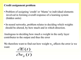
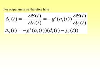
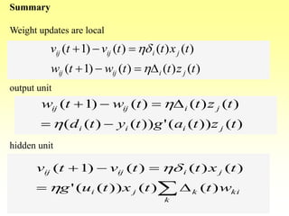
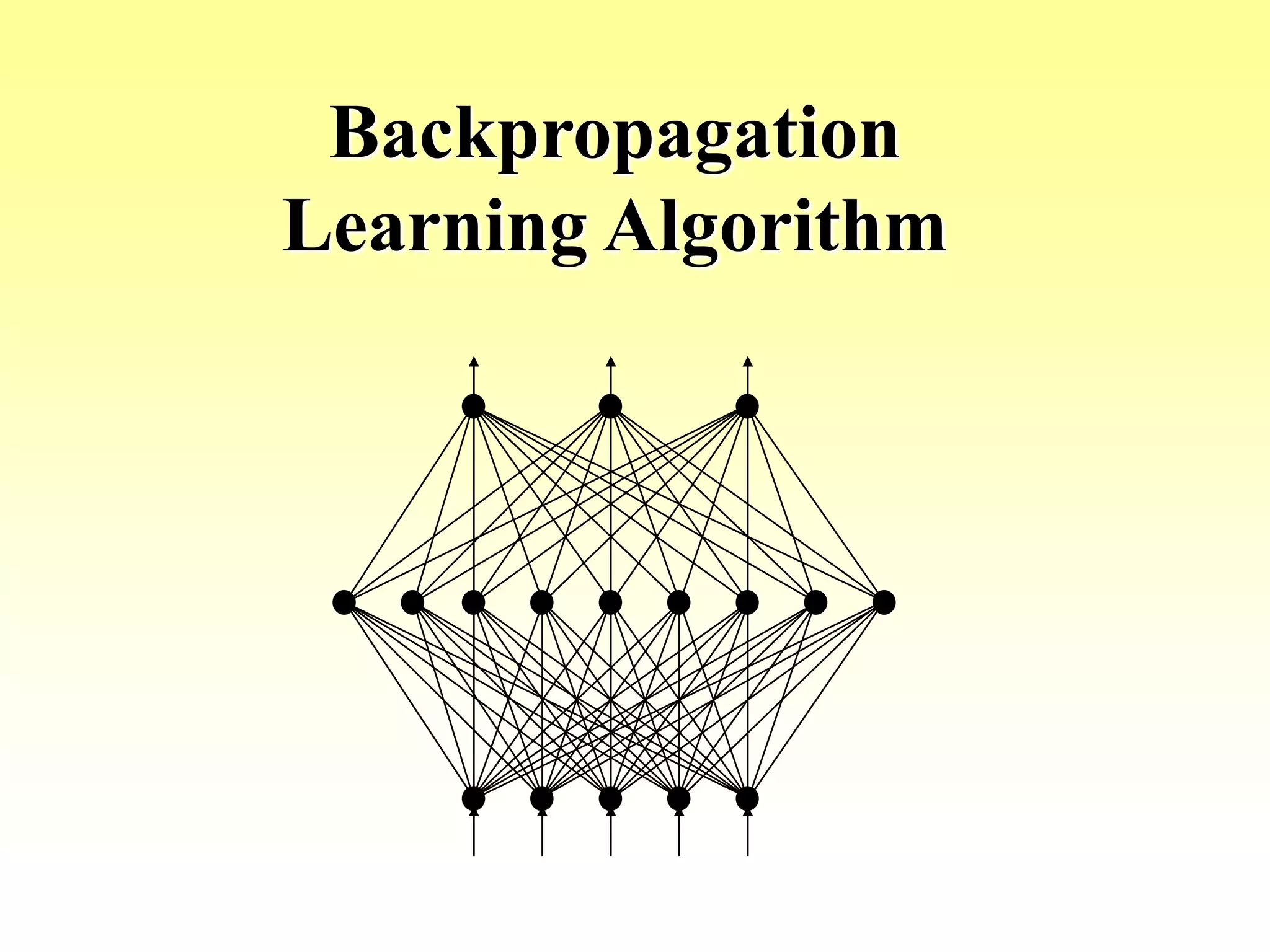
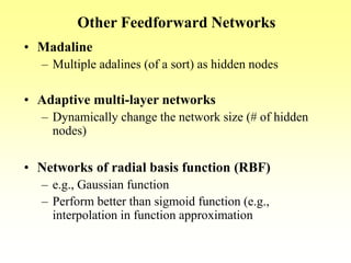
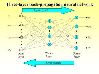
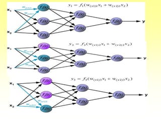
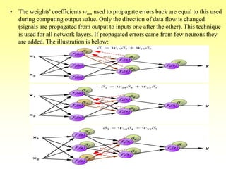
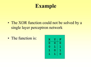
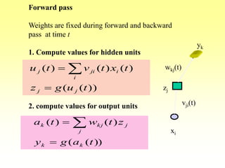
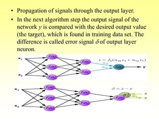
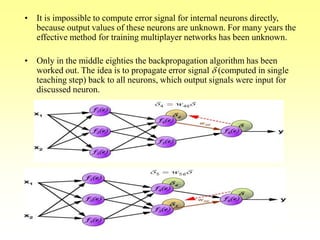
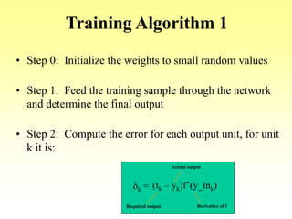
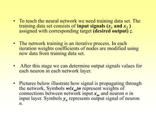
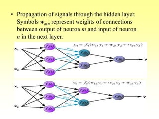
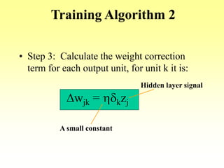
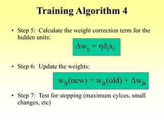
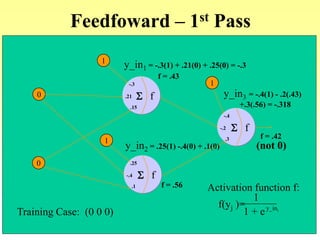
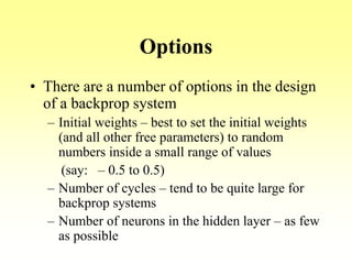
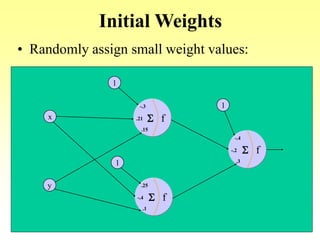
The document provides an overview of backpropagation, a common algorithm used to train multi-layer neural networks. It discusses: - How backpropagation works by calculating error terms for output nodes and propagating these errors back through the network to adjust weights. - The stages of feedforward activation and backpropagation of errors to update weights. - Options like initial random weights, number of training cycles and hidden nodes. 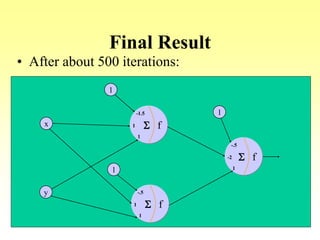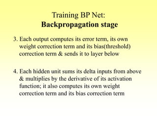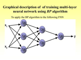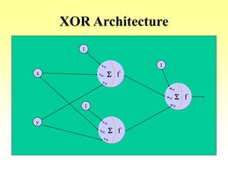- An example of using backpropagation to train a network to learn the XOR function over multiple training passes of forward passing and backward error propagation and weight updating.

1. Backpropagation
Learning Algorithm

2. The backpropagation algorithm was used to train the
multi layer perception MLP
MLP used to describe any general Feedforward (no
recurrent connections) Neural Network FNN
However, we will concentrate on nets with units
arranged in layers
x1
xn

3. Architecture of BP Nets
• Multi-layer, feed-forward networks have the following
characteristics:
-They must have at least one hidden layer
– Hidden units must be non-linear units (usually with sigmoid
activation functions)
– Fully connected between units in two consecutive layers, but no
connection between units within one layer.
– For a net with only one hidden layer, each hidden unit receives
input from all input units and sends output to all output units
– Number of output units need not equal number of input units
– Number of hidden units per layer can be more or less than
input or output units

4. Other Feedforward Networks
• Madaline
– Multiple adalines (of a sort) as hidden nodes
• Adaptive multi-layer networks
– Dynamically change the network size (# of hidden
nodes)
• Networks of radial basis function (RBF)
– e.g., Gaussian function
– Perform better than sigmoid function (e.g.,
interpolation in function approximation

5. Introduction to Backpropagation
• In 1969 a method for learning in multi-layer network,
Backpropagation (or generalized delta rule) , was invented by
Bryson and Ho.
• It is best-known example of a training algorithm. Uses training
data to adjust weights and thresholds of neurons so as to
minimize the networks errors of prediction.
• Slower than gradient descent .
• Easiest algorithm to understand
• Backpropagation works by applying the gradient descent
rule to a feedforward network.

6. • How many hidden layers and hidden units per layer?
– Theoretically, one hidden layer (possibly with many
hidden units) is sufficient for any L2 functions
– There is no theoretical results on minimum necessary #
of hidden units (either problem dependent or
independent)
– Practical rule :
•n = # of input units; p = # of hidden units
•For binary/bipolar data: p = 2n
•For real data: p >> 2n
– Multiple hidden layers with fewer units may be trained
faster for similar quality in some applications

7. Training a BackPropagation Net
• Feedforward training of input patterns
– each input node receives a signal, which is broadcast to all of the
hidden units
– each hidden unit computes its activation which is broadcast to all
output nodes
• Back propagation of errors
– each output node compares its activation with the desired output
– based on these differences, the error is propagated back to all
previous nodes Delta Rule
• Adjustment of weights
– weights of all links computed simultaneously based on the errors
that were propagated back

8. Three-layer back-propagation neural network
Input
layer
xi
x1
x2
xn
1
2
i
n
Output
layer
1
2
k
l
yk
y1
y2
yl
Input signals
Error signals
wjk
Hidden
layer
wij
1
2
j
m

9. Generalized delta rule
• Delta rule only works for the output layer.
• Backpropagation, or the generalized delta
rule, is a way of creating desired values for
hidden layers

10. Description of Training BP Net:
Feedforward Stage
1. Initialize weights with small, random values
2. While stopping condition is not true
– for each training pair (input/output):
• each input unit broadcasts its value to all hidden
units
• each hidden unit sums its input signals & applies
activation function to compute its output signal
• each hidden unit sends its signal to the output units
• each output unit sums its input signals & applies its
activation function to compute its output signal

11. Training BP Net:
Backpropagation stage
3. Each output computes its error term, its own
weight correction term and its bias(threshold)
correction term & sends it to layer below
4. Each hidden unit sums its delta inputs from above
& multiplies by the derivative of its activation
function; it also computes its own weight
correction term and its bias correction term

12. Training a Back Prop Net:
Adjusting the Weights
5. Each output unit updates its weights and bias
6. Each hidden unit updates its weights and bias
– Each training cycle is called an epoch. The
weights are updated in each cycle
– It is not analytically possible to determine where
the global minimum is. Eventually the algorithm
stops in a low point, which may just be a local
minimum.

13. How long should you train?
• Goal: balance between correct responses for
training patterns & correct responses for new
patterns (memorization v. generalization)
• In general, network is trained until it reaches an
acceptable error rate (e.g. 95%)
• If train too long, you run the risk of overfitting

14. Graphical description of of training multi-layer
neural network using BP algorithm
To apply the BP algorithm to the following FNN

15. • To teach the neural network we need training data set. The
training data set consists of input signals (x1 and x2 )
assigned with corresponding target (desired output) z.
• The network training is an iterative process. In each
iteration weights coefficients of nodes are modified using
new data from training data set.
• After this stage we can determine output signals values for
each neuron in each network layer.
• Pictures below illustrate how signal is propagating through
the network, Symbols w(xm)n represent weights of
connections between network input xm and neuron n in
input layer. Symbols yn represents output signal of neuron
n.

17. • Propagation of signals through the hidden layer.
Symbols wmn represent weights of connections
between output of neuron m and input of neuron
n in the next layer.

18. • Propagation of signals through the output layer.
• In the next algorithm step the output signal of the
network y is compared with the desired output value
(the target), which is found in training data set. The
difference is called error signal d of output layer
neuron.

19. • It is impossible to compute error signal for internal neurons directly,
because output values of these neurons are unknown. For many years the
effective method for training multiplayer networks has been unknown.
• Only in the middle eighties the backpropagation algorithm has been
worked out. The idea is to propagate error signal d (computed in single
teaching step) back to all neurons, which output signals were input for
discussed neuron.

20. • The weights' coefficients wmn used to propagate errors back are equal to this used
during computing output value. Only the direction of data flow is changed
(signals are propagated from output to inputs one after the other). This technique
is used for all network layers. If propagated errors came from few neurons they
are added. The illustration is below:

21. • When the error
signal for each
neuron is
computed, the
weights
coefficients of
each neuron input
node may be
modified. In
formulas below
df(e)/de represents
derivative of
neuron activation
function (which
weights are
modified).

23. Coefficient h affects network teaching speed. There are a few techniques
to select this parameter. The first method is to start teaching process with
large value of the parameter. While weights coefficients are being
established the parameter is being decreased gradually.
The second, more complicated, method starts teaching with small
parameter value. During the teaching process the parameter is being
increased when the teaching is advanced and then decreased again in the
final stage.

24. Training Algorithm 1
• Step 0: Initialize the weights to small random values
• Step 1: Feed the training sample through the network
and determine the final output
• Step 2: Compute the error for each output unit, for unit
k it is:
dk = (tk – yk)f’(y_ink)
Required output
Actual output
Derivative of f

25. Training Algorithm 2
• Step 3: Calculate the weight correction
term for each output unit, for unit k it is:
Dwjk = hdkzj
A small constant
Hidden layer signal

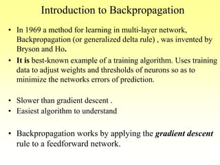
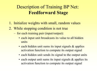
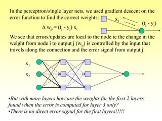
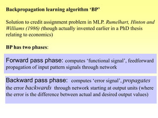
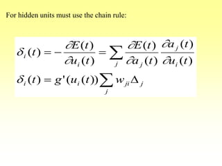
26. Training Algorithm 3
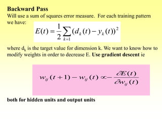
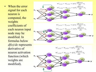
• Step 4: Propagate the delta terms (errors) back
through the weights of the hidden units where
the delta input for the jth hidden unit is:
d_inj =
dkwjk
Sk=1
m
The delta term for the jth hidden unit is:
dj = d_injf’(z_inj)
where
f’(z_inj)= f(z_inj)[1- f(z_inj)]

27. Training Algorithm 4
• Step 5: Calculate the weight correction term for the
hidden units:
• Step 6: Update the weights:
• Step 7: Test for stopping (maximum cylces, small
changes, etc)
Dwij = hdjxi
wjk(new) = wjk(old) + Dwjk

28. Options
• There are a number of options in the design
of a backprop system
– Initial weights – best to set the initial weights
(and all other free parameters) to random
numbers inside a small range of values
(say: – 0.5 to 0.5)
– Number of cycles – tend to be quite large for
backprop systems
– Number of neurons in the hidden layer – as few
as possible

29. Example
• The XOR function could not be solved by a
single layer perceptron network
• The function is: X Y F
0 0 0
0 1 1
1 0 1
1 1 0

30. XOR Architecture
x
y
fv21 S
v11
v31
fv22 S
v12
v32
fw21 S
w11
w31
1
1
1

31. Initial Weights
• Randomly assign small weight values:
x
y
f.21 S
-.3
.15
f-.4 S
.25
.1
f-.2 S
-.4
.3
1
1
1

32. Feedfoward – 1st Pass
x
y
f.21 S
-.3
.15
f-.4 S
.25
.1
f-.2 S
-.4
.3
1
1
1
Training Case: (0 0 0)
0
0
1
1
y_in1 = -.3(1) + .21(0) + .25(0) = -.3
f(yj )= y_ini
1
1 + e
Activation function f:
f = .43
y_in2 = .25(1) -.4(0) + .1(0)
f = .56
1
y_in3 = -.4(1) - .2(.43)
+.3(.56) = -.318
f = .42
(not 0)

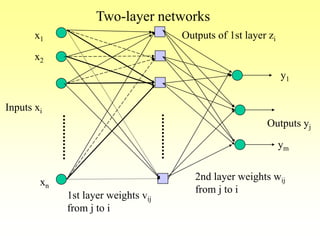
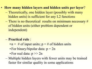
33. Backpropagate
0
0
f.21 S
-.3
.15
f-.4 S
.25
.1
f-.2 S
-.4
.3
1
1
1
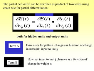
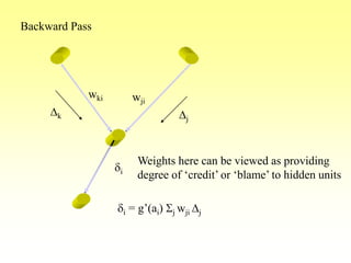
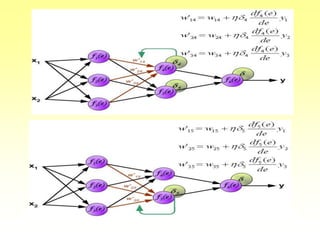
d3 = (t3 – y3)f’(y_in3)
=(t3 – y3)f(y_in3)[1- f(y_in3)]
d3 = (0 – .42).42[1-.42]
= -.102
d_in1 = d3w13 = -.102(-.2) = .02
d1 = d_in1f’(z_in1) = .02(.43)(1-.43)
= .005
d_in2 = d3w12 = -.102(.3) = -.03
d2 = d_in2f’(z_in2) = -.03(.56)(1-.56)
= -.007

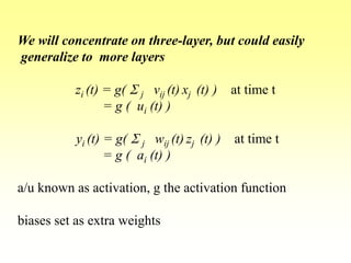
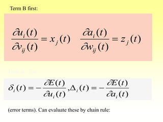
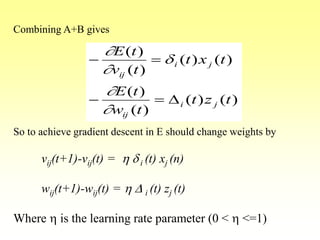
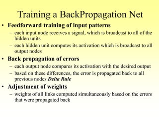
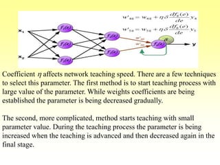
34. Update the Weights – First Pass
0
0
f.21 S
-.3
.15
f-.4 S
.25
.1
f-.2 S
-.4
.3
1
1
1
d3 = (t3 – y3)f’(y_in3)
=(t3 – y3)f(y_in3)[1- f(y_in3)]
d3 = (0 – .42).42[1-.42]
= -.102
d_in1 = d3w13 = -.102(-.2) = .02
d1 = d_in1f’(z_in1) = .02(.43)(1-.43)
= .005
d_in2 = d3w12 = -.102(.3) = -.03
d2 = d_in2f’(z_in2) = -.03(.56)(1-.56)
= -.007

35. Final Result
• After about 500 iterations:
x
y
f1 S
-1.5
1
f1 S
-.5
1
f-2 S
-.5
1
1
1
1

36. More details for
gradient descent method + MLP
to whom may have interest

37. In the perceptron/single layer nets, we used gradient descent on the
error function to find the correct weights:
D wji = (tj - yj) xi
We see that errors/updates are local to the node ie the change in the
weight from node i to output j (wji) is controlled by the input that
travels along the connection and the error signal from output j
x1
x2
•But with more layers how are the weights for the first 2 layers
found when the error is computed for layer 3 only?
•There is no direct error signal for the first layers!!!!!
?
x1
(tj - yj)

38. Credit assignment problem
• Problem of assigning ‘credit’ or ‘blame’ to individual elements
involved in forming overall response of a learning system
(hidden units)
• In neural networks, problem relates to deciding which weights
should be altered, by how much and in which direction.
Analogous to deciding how much a weight in the early layer
contributes to the output and thus the error
We therefore want to find out how weight wij affects the error ie we
want:
)(
)(
tw
tE
ij


39. Backpropagation learning algorithm ‘BP’
Solution to credit assignment problem in MLP
Rumelhart, Hinton and Williams (1986)
BP has two phases:
Forward pass phase: computes ‘functional signal’, feedforward
propagation of input pattern signals through
network

40. Backpropagation learning algorithm ‘BP’
Solution to credit assignment problem in MLP. Rumelhart, Hinton and
Williams (1986) (though actually invented earlier in a PhD thesis
relating to economics)
BP has two phases:
Forward pass phase: computes ‘functional signal’, feedforward
propagation of input pattern signals through network
Backward pass phase: computes ‘error signal’, propagates
the error backwards through network starting at output units (where
the error is the difference between actual and desired output values)

41. xn
x1
x2
Inputs xi
Outputs yj
Two-layer networks
y1
ym
2nd layer weights wij
from j to i
1st layer weights vij
from j to i
Outputs of 1st layer zi

42. We will concentrate on three-layer, but could easily
generalize to more layers
zi (t) = g( S j vij (t) xj (t) ) at time t
= g ( ui (t) )
yi (t) = g( S j wij (t) zj (t) ) at time t
= g ( ai (t) )
a/u known as activation, g the activation function
biases set as extra weights

43. Forward pass
Weights are fixed during forward and backward
pass at time t
1. Compute values for hidden units
2. compute values for output units
))((
)()()(
tugz
txtvtu
jj
i
ijij

 
))((
)()(
tagy
ztwta
kk
j
jkjk

 
xi
vji(t)
wkj(t)
zj
yk

44. Backward Pass
Will use a sum of squares error measure. For each training pattern
we have:
where dk is the target value for dimension k. We want to know how to
modify weights in order to decrease E. Use gradient descent ie
both for hidden units and output units


1
2
))()((
2
1
)(
k
kk tytdtE
)(
)(
)()1(
tw
tE
twtw
ij
ijij




45. )(
)(
)(
)(
)(
)(
tw
ta
ta
tE
tw
tE
ij
i
iij 






How error for pattern changes as function of change
in network input to unit j
How net input to unit j changes as a function of
change in weight w
both for hidden units and output units
Term A
Term B
The partial derivative can be rewritten as product of two terms using
chain rule for partial differentiation

46. Term A Let
)(
)(
)(,
)(
)(
)(
ta
tE
t
tu
tE
t
i
i
i
i




d D
(error terms). Can evaluate these by chain rule:
)(
)(
)(
)(
)(
)(
tz
tw
ta
tx
tv
tu
j
ij
i
j
ij
i





Term B first:

47. ))()())(((')(
)(
)(
))(('
)(
)(
)(
tytdtagt
ty
tE
tag
ta
tE
t
iiii
i
i
i
i
D
D




For output units we therefore have:

48. 

D

j
jjiii
i
j
j ji
i
wtugt
tu
ta
ta
tE
tu
tE
t
))((')(
)(
)(
)(
)(
)(
)(
)(
d






d
For hidden units must use the chain rule:

49. Backward Pass
Weights here can be viewed as providing
degree of ‘credit’ or ‘blame’ to hidden units
Dj
Dk
di
wki wji
di = g’(ai) Sj wji Dj

50. Combining A+B gives
So to achieve gradient descent in E should change weights by
vij(t+1)-vij(t) = h d i (t) xj (n)
wij(t+1)-wij(t) = h D i (t) zj (t)
Where h is the learning rate parameter (0 < h <=1)
)()(
)(
)(
)()(
)(
)(
tzt
tw
tE
txt
tv
tE
ji
ij
ji
ij
D



d



51. Summary
Weight updates are local
output unit
hidden unit
)()()()1(
)()()()1(
tzttwtw
txttvtv
jiijij
jiijij
D

h
hd
D

k
kikji
jiijij
wttxtug
txttvtv
)()())(('
)()()()1(
h
hd
)())(('))()((
)()()()1(
tztagtytd
tzttwtw
jiii
jiijij

D
h
h

52. End of slides