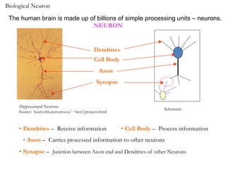
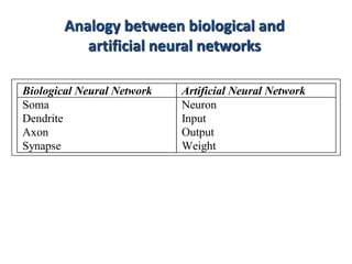
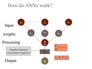
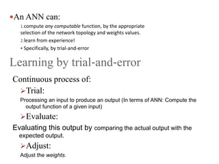
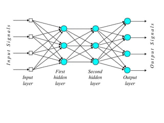
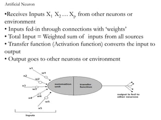
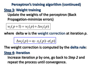
1. Neural networks are inspired by biological neural networks in the brain and are made up of simple processing units called neurons. 2. Artificial neural networks use a layer of input neurons that receive information and pass it through connections to other neurons. 3. A neural network learns through a process of trial and error adjustment of the weights between neurons to minimize errors between the network's output and the desired output.

1. Presented by Rauf Asadov
Neural Networks

2. The human brain is made up of billions of simple processing units – neurons.
NEURON
• Dendrites – Receive information
Biological Neuron
Hippocampal Neurons
Source: heart.cbl.utoronto.ca/ ~berj/projects.html
• Cell Body – Process information
• Axon – Carries processed information to other neurons
• Synapse – Junction between Axon end and Dendrites of other Neurons
Dendrites
Cell Body
Axon
Schematic
Synapse

4. Artificial Neuron
•Receives Inputs X1 X2 … Xp from other neurons or
environment
• Inputs fed-in through connections with ‘weights’
• Total Input = Weighted sum of inputs from all sources
• Transfer function (Activation function) converts the input to
output
• Output goes to other neurons or environment

5. Biological Neural Network Artificial Neural Network
Soma
Dendrite
Axon
Synapse
Neuron
Input
Output
Weight
Analogy between biological and
artificial neural networks

6. How do ANNs work?
Transfer Function
(Activation Function)
Output
x1x2xm
∑
y
Processing
Input
w1
w2wm
weights
. . . . . . . . . .
. .
f(vk)
. . . .
.

7. Activation functions of a neuron
Step function Sign function
+1
-1
0
+1
-1
0X
Y
X
Y
+1
-1
0 X
Y
Sigmoid function
+1
-1
0 X
Y
Linear function






0if,0
0if,1
X
X
Ystep






0if,1
0if,1
X
X
Y sign
X
sigmoid
e
Y


1
1 XY linear


8.  The neuron computes the weighted sum of the input
signals and compares the result with a threshold
value, . If the net input is less than the threshold,
the neuron output is –1. But if the net input is
greater than or equal to the threshold, the neuron
becomes activated and its output attains a value +1.
 The neuron uses the following transfer or activation
function:
 This type of activation function is called a sign
function.



n
i
iiwxX
1 





X
X
Y
if,1
if,1

9. Can a single neuron learn a task?
 In 1958, Frank Rosenblatt introduced a training
algorithm that provided the first procedure for
training a simple ANN: a perceptron.
 The perceptron is the simplest form of a neural
network. It consists of a single neuron with
adjustable synaptic weights and a hard limiter.

10. Threshold
Inputs
x1
x2
Output
Y
Hard
Limiter
w2
w1
Linear
Combiner

Single-layer two-input perceptron

11. 11
Perceptron
• Is a network with all inputs connected directly to the output.
This is called a single layer NN (Neural Network) or a
Perceptron Network.
• A perceptron is a single neuron that classifies a set of inputs into
one of two categories (usually 1 or -1)
• If the inputs are in the form of a grid, a perceptron can be used to
recognize visual images of shapes.
• The perceptron usually uses a step function, which returns 1 if the
weighted sum of inputs exceeds a threshold, and –1 otherwise.
 The operation of Rosenblatt’s perceptron is based on the
McCulloch and Pitts neuron model. The model consists of a
linear combiner followed by a hard limiter.
 The weighted sum of the inputs is applied to the hard limiter,
which produces an output equal to +1 if its input is positive and
1 if it is negative.

12. An ANN can:
1.compute any computable function, by the appropriate
selection of the network topology and weights values.
2.learn from experience!
 Specifically, by trial‐and‐error
Learning by trial‐and‐error
Continuous process of:
Trial:
Processing an input to produce an output (In terms of ANN: Compute the
output function of a given input)
Evaluate:
Evaluating this output by comparing the actual output with the
expected output.
Adjust:
Adjust the weights.

13. x2
x1
??
Or hyperplane in
n-dimensional space
x2= mx1+q
Perceptron learns a linear separator
This is an (hyper)-line in an n-dimensional
space, what is learnt
are the coefficients wi
Instances X(x1,x2..x2) such that:
Are classified as positive, else they are classified as
negative

14. Perceptron Training- Preparation
• First, inputs are given random weights (usually
between –0.5 and 0.5)
• In the case of an elementary perceptron, the n-
dimensional space is divided by a hyperplane
into two decision regions. (i.e If we have 2
results we can separate them with a line with
each group result on a different side of the line)
The hyperplane is defined by the linearly
separable function:
0
1


n
i
iiwx

15.  If at iteration p, the actual output is Y(p) and the
desired output is Yd (p), then the error is given by:
where p = 1, 2, 3, . . .
Iteration p here refers to the pth training example
presented to the perceptron.
 If the error, e(p), is positive, we need to increase
perceptron output Y(p), but if it is negative, we
need to decrease Y(p).
)()()( pYpYpe d 

16. The perceptron learning formula
where p = 1, 2, 3, . . .
 is the learning rate, a positive constant less than
unity.
)()()()1( pepxpwpw iii  

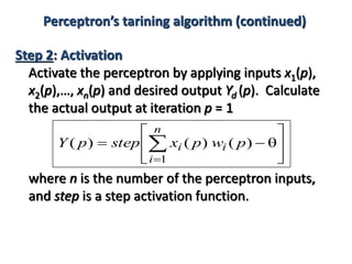
17. Step 1: Initialisation
Set initial weights w1, w2,…, wn and threshold 
to random numbers in the range [0.5, 0.5].
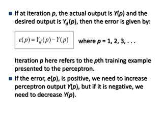
If the error, e(p), is positive, we need to increase
perceptron output Y(p), but if it is negative, we
need to decrease Y(p).
Perceptron’s training algorithm

18. Step 2: Activation
Activate the perceptron by applying inputs x1(p),
x2(p),…, xn(p) and desired output Yd (p). Calculate
the actual output at iteration p = 1
where n is the number of the perceptron inputs,
and step is a step activation function.
Perceptron’s tarining algorithm (continued)








 

n
i
ii pwpxsteppY
1
)()()(

19. Step 3: Weight training
Update the weights of the perceptron (Back
Propagation-minimize errors)
where delta w is the weight correction at iteration p.
The weight correction is computed by the delta rule:
Step 4: Iteration
Increase iteration p by one, go back to Step 2 and
repeat the process until convergence.
)()()1( pwpwpw iii 
Perceptron’s training algorithm (continued)
)()()( pepxpw ii 

20. X1
X2
W1
W2
X1 X2 Y Train
0 0 0
0 1 0
1 0 0
1 1 1
Perceptron’s training for AND logic gate
∑
Activation function

21. Example of perceptron learning: the logical operation AND
Inputs
x1 x2
0
0
1
1
0
1
0
1
0
0
0
Epoch
Desired
output
Yd
1
Initial
weights
w1 w2
1
0.3
0.3
0.3
0.2
0.1
0.1
0.1
0.1
0
0
1
0
Actual
output
Y
Error
e
0
0
1
1
Final
weights
w1 w2
0.3
0.3
0.2
0.3
0.1
0.1
0.1
0.0
0
0
1
1
0
1
0
1
0
0
0
2
1
0.3
0.3
0.3
0.2
0
0
1
1
0
0
1
0
0.3
0.3
0.2
0.2
0.0
0.0
0.0
0.0
0
0
1
1
0
1
0
1
0
0
0
3
1
0.2
0.2
0.2
0.1
0.0
0.0
0.0
0.0
0.0
0.0
0.0
0.0
0
0
1
0
0
0
1
1
0.2
0.2
0.1
0.2
0.0
0.0
0.0
0.1
0
0
1
1
0
1
0
1
0
0
0
4
1
0.2
0.2
0.2
0.1
0.1
0.1
0.1
0.1
0
0
1
1
0
0
1
0
0.2
0.2
0.1
0.1
0.1
0.1
0.1
0.1
0
0
1
1
0
1
0
1
0
0
0
5
1
0.1
0.1
0.1
0.1
0.1
0.1
0.1
0.1
0
0
0
1
0
0
0
0.1
0.1
0.1
0.1
0.1
0.1
0.1
0.1
0
Threshold:  = 0.2; learning rate:  = 0.1

22. Multilayer Perceptron
 A multilayer perceptron neural network
with one or more hidden layers.
 Hierarchical structure
 The network consists of an input layer of
source neurons, at least one middle or
hidden layer of computational neurons,
and an output layer of computational
neurons.

23. Input
layer
First
hidden
layer
Second
hidden
layer
Output
layer
OutputSignals
InputSignals

24. What does the middle layer hide?
 A hidden layer “hides” its desired output. Neurons
in the hidden layer cannot be observed through the
input/output behaviour of the network. There is no
obvious way to know what the desired output of
the hidden layer should be.
 Commercial ANNs incorporate three and sometimes
four layers, including one or two hidden layers.
Each layer can contain from 10 to 1000 neurons.
Experimental neural networks may have five or
even six layers, including three or four hidden
layers, and utilise millions of neurons.

25. Learning Paradigms
Supervised learning
Unsupervised learning
Reinforcement learning
In artificial neural networks, learning refers to the
method of modifying the weights of connections
between the nodes of a specified network.

26. Supervised learning
 This is what we have seen so far!
 A network is fed with a set of training samples
(inputs and corresponding output), and it uses
these samples to learn the general relationship
between the inputs and the outputs.
 This relationship is represented by the values of
the weights of the trained network.

27. Unsupervised learning
 No desired output is associated with the
training data!
 Faster than supervised learning
 Used to find out structures within data:
 Clustering
 Compression

28. Reinforcement learning
 Like supervised learning, but:
 Weights adjusting is not directly related to the error
value.
 The error value is used to randomly, shuffle weights!
 Relatively slow learning due to ‘randomness’.