Study material with basic information and worked out example on XOR problem

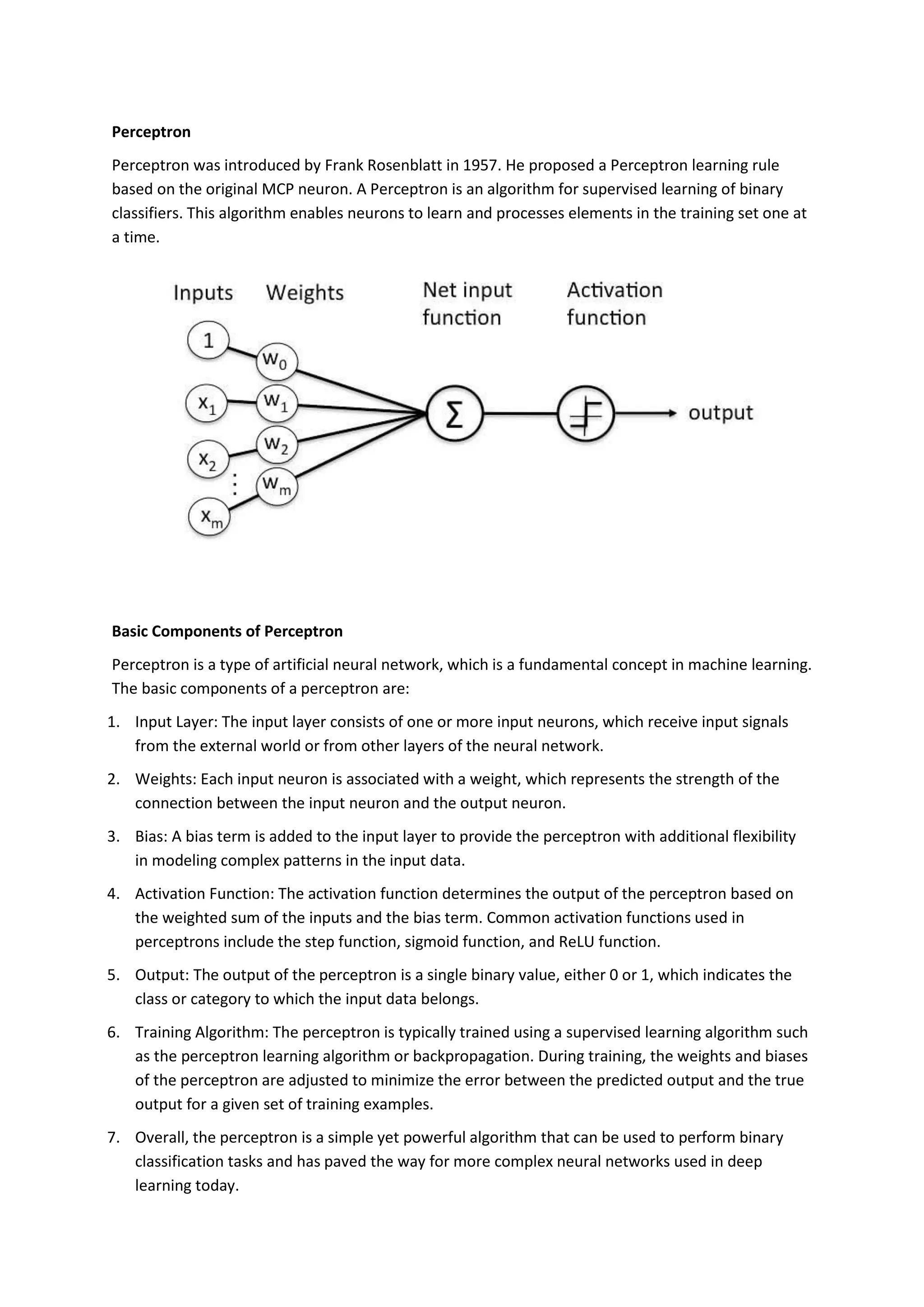
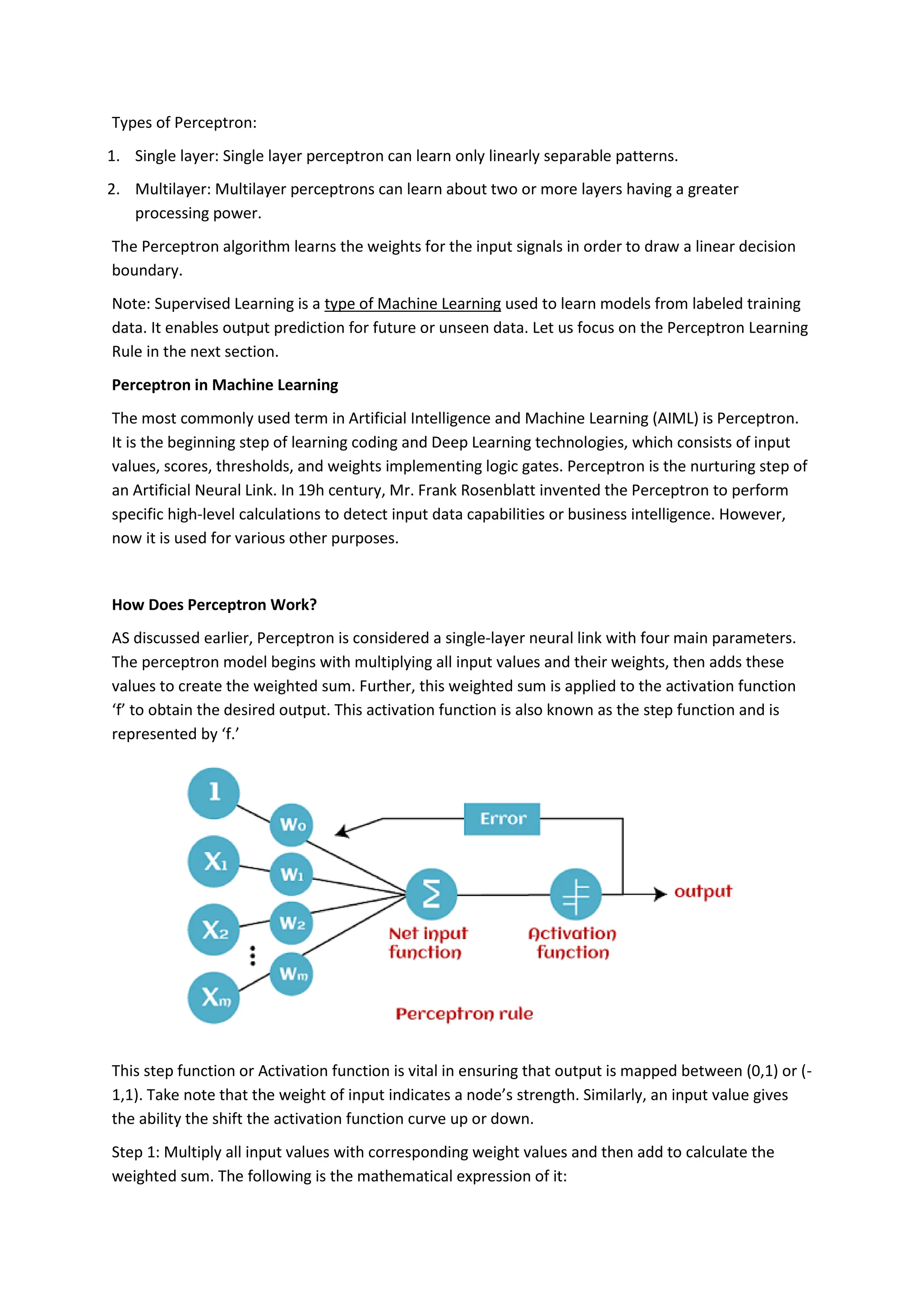
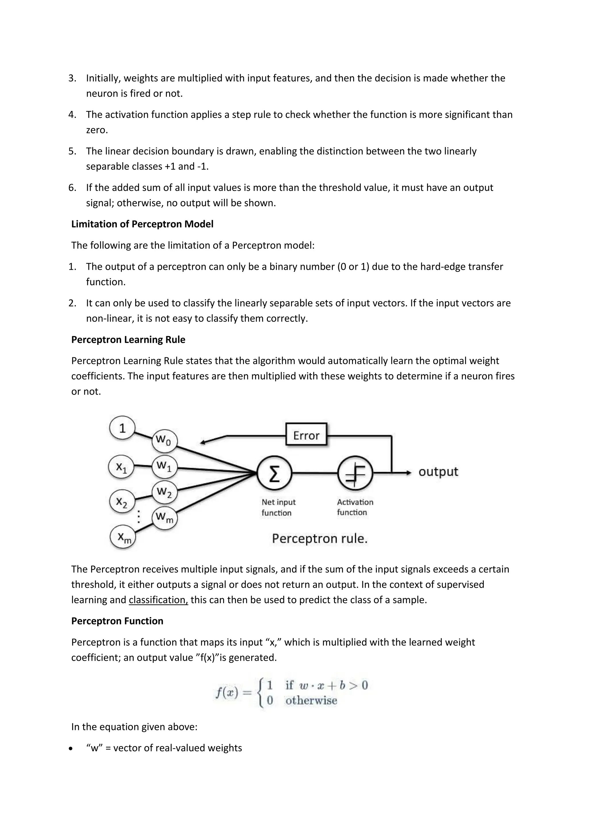
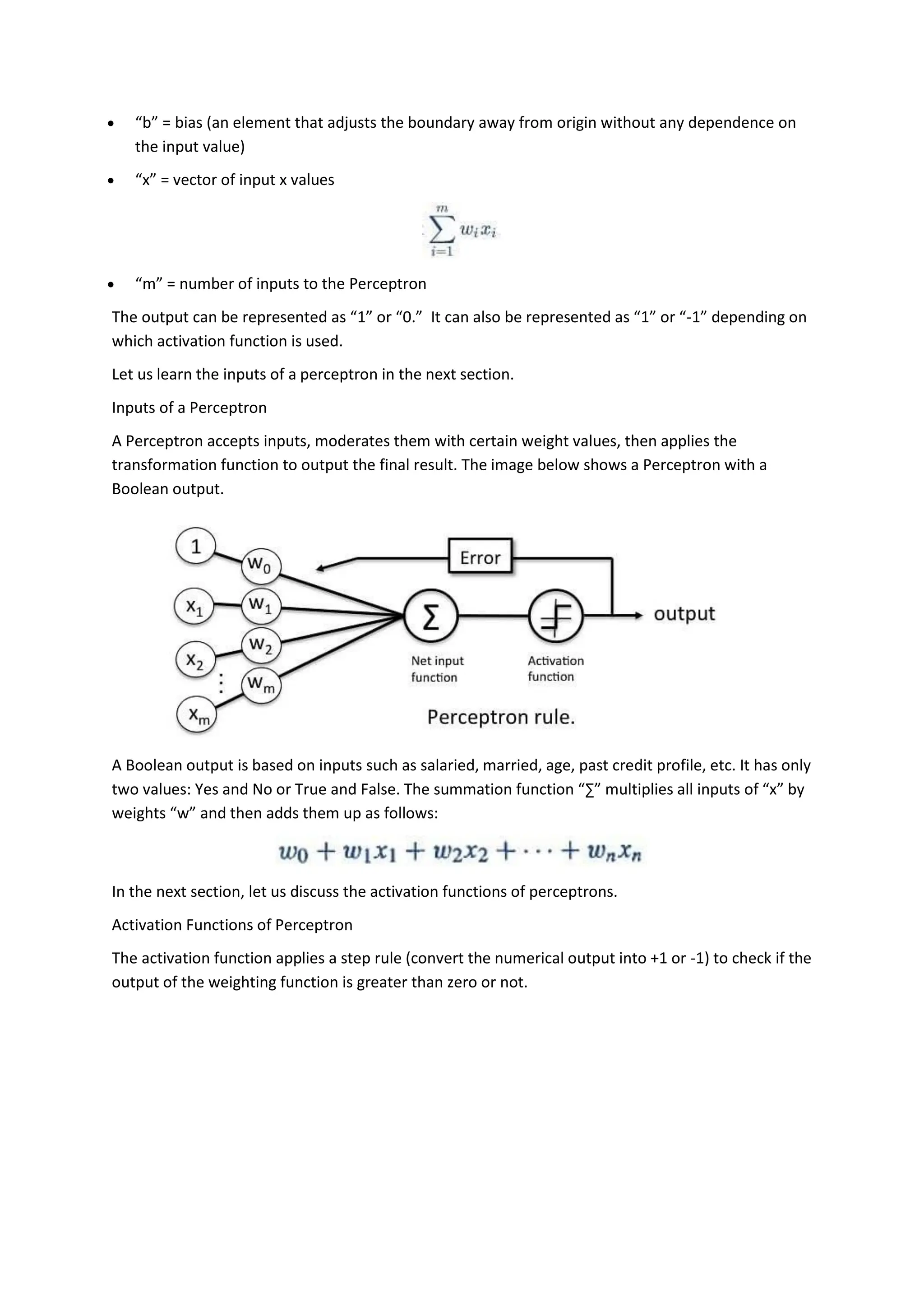
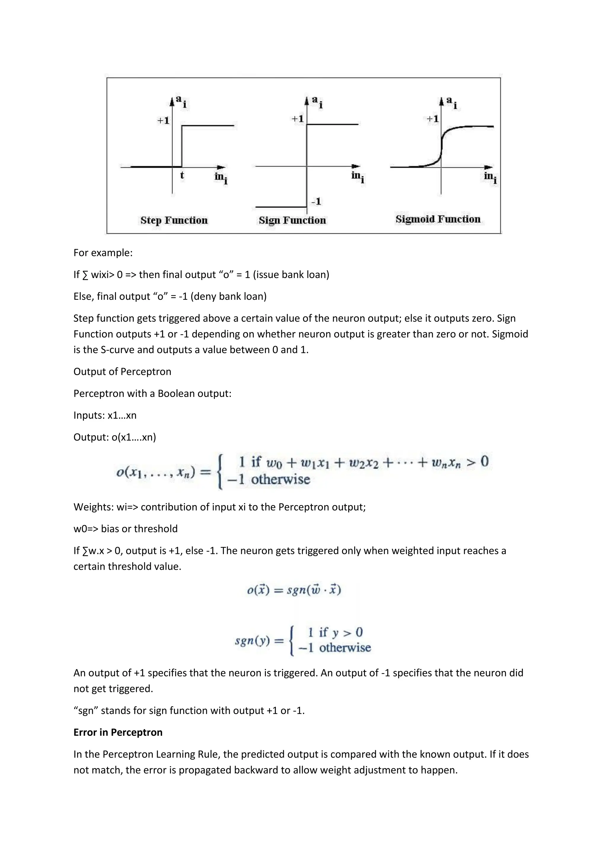
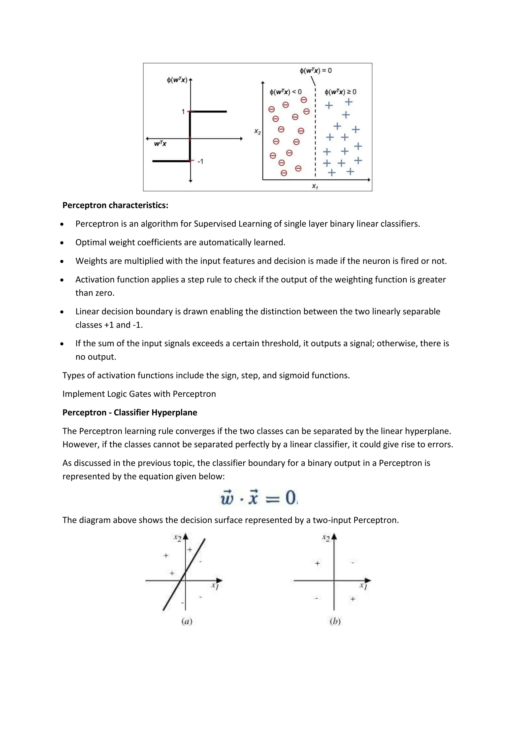
1. Perceptron
Perceptron was introduced by Frank Rosenblatt in 1957. He proposed a Perceptron learning rule
based on the original MCP neuron. A Perceptron is an algorithm for supervised learning of binary
classifiers. This algorithm enables neurons to learn and processes elements in the training set one at
a time.
Basic Components of Perceptron
Perceptron is a type of artificial neural network, which is a fundamental concept in machine learning.
The basic components of a perceptron are:
1. Input Layer: The input layer consists of one or more input neurons, which receive input signals
from the external world or from other layers of the neural network.
2. Weights: Each input neuron is associated with a weight, which represents the strength of the
connection between the input neuron and the output neuron.
3. Bias: A bias term is added to the input layer to provide the perceptron with additional flexibility
in modeling complex patterns in the input data.
4. Activation Function: The activation function determines the output of the perceptron based on
the weighted sum of the inputs and the bias term. Common activation functions used in
perceptrons include the step function, sigmoid function, and ReLU function.
5. Output: The output of the perceptron is a single binary value, either 0 or 1, which indicates the
class or category to which the input data belongs.
6. Training Algorithm: The perceptron is typically trained using a supervised learning algorithm such
as the perceptron learning algorithm or backpropagation. During training, the weights and biases
of the perceptron are adjusted to minimize the error between the predicted output and the true
output for a given set of training examples.
7. Overall, the perceptron is a simple yet powerful algorithm that can be used to perform binary
classification tasks and has paved the way for more complex neural networks used in deep
learning today.

2. Types of Perceptron:
1. Single layer: Single layer perceptron can learn only linearly separable patterns.
2. Multilayer: Multilayer perceptrons can learn about two or more layers having a greater
processing power.
The Perceptron algorithm learns the weights for the input signals in order to draw a linear decision
boundary.
Note: Supervised Learning is a type of Machine Learning used to learn models from labeled training
data. It enables output prediction for future or unseen data. Let us focus on the Perceptron Learning
Rule in the next section.
Perceptron in Machine Learning
The most commonly used term in Artificial Intelligence and Machine Learning (AIML) is Perceptron.
It is the beginning step of learning coding and Deep Learning technologies, which consists of input
values, scores, thresholds, and weights implementing logic gates. Perceptron is the nurturing step of
an Artificial Neural Link. In 19h century, Mr. Frank Rosenblatt invented the Perceptron to perform
specific high-level calculations to detect input data capabilities or business intelligence. However,
now it is used for various other purposes.
How Does Perceptron Work?
AS discussed earlier, Perceptron is considered a single-layer neural link with four main parameters.
The perceptron model begins with multiplying all input values and their weights, then adds these
values to create the weighted sum. Further, this weighted sum is applied to the activation function
‘f’ to obtain the desired output. This activation function is also known as the step function and is
represented by ‘f.’
This step function or Activation function is vital in ensuring that output is mapped between (0,1) or (-
1,1). Take note that the weight of input indicates a node’s strength. Similarly, an input value gives
the ability the shift the activation function curve up or down.
Step 1: Multiply all input values with corresponding weight values and then add to calculate the
weighted sum. The following is the mathematical expression of it:

3. ∑wi*xi = x1*w1 + x2*w2 + x3*w3+……..x4*w4
Add a term called bias ‘b’ to this weighted sum to improve the model’s performance.
Step 2: An activation function is applied with the above-mentioned weighted sum giving us an
output either in binary form or a continuous value as follows:
Y=f(∑wi*xi + b)
Types of Perceptron models
We have already discussed the types of Perceptron models in the Introduction. Here, we shall give a
more profound look at this:
1. Single Layer Perceptron model: One of the easiest ANN (Artificial Neural Networks) types consists
of a feed-forward network and includes a threshold transfer inside the model. The main objective
of the single-layer perceptron model is to analyze the linearly separable objects with binary
outcomes. A Single-layer perceptron can learn only linearly separable patterns.
2. Multi-Layered Perceptron model: It is mainly similar to a single-layer perceptron model but has
more hidden layers.
Forward Stage: From the input layer in the on stage, activation functions begin and terminate on the
output layer.
Backward Stage: In the backward stage, weight and bias values are modified per the model’s
requirement. The backstage removed the error between the actual output and demands originating
backward on the output layer. A multilayer perceptron model has a greater processing power and
can process linear and non-linear patterns. Further, it also implements logic gates such as AND, OR,
XOR, XNOR, and NOR.
Advantages:
 A multi-layered perceptron model can solve complex non-linear problems.
 It works well with both small and large input data.
 Helps us to obtain quick predictions after the training.
 Helps us obtain the same accuracy ratio with big and small data.
Disadvantages:
 In multi-layered perceptron model, computations are time-consuming and complex.
 It is tough to predict how much the dependent variable affects each independent variable.
 The model functioning depends on the quality of training.
Characteristics of the Perceptron Model
The following are the characteristics of a Perceptron Model:
1. It is a machine learning algorithm that uses supervised learning of binary classifiers.
2. In Perceptron, the weight coefficient is automatically learned.

4. 3. Initially, weights are multiplied with input features, and then the decision is made whether the
neuron is fired or not.
4. The activation function applies a step rule to check whether the function is more significant than
zero.
5. The linear decision boundary is drawn, enabling the distinction between the two linearly
separable classes +1 and -1.
6. If the added sum of all input values is more than the threshold value, it must have an output
signal; otherwise, no output will be shown.
Limitation of Perceptron Model
The following are the limitation of a Perceptron model:
1. The output of a perceptron can only be a binary number (0 or 1) due to the hard-edge transfer
function.
2. It can only be used to classify the linearly separable sets of input vectors. If the input vectors are
non-linear, it is not easy to classify them correctly.
Perceptron Learning Rule
Perceptron Learning Rule states that the algorithm would automatically learn the optimal weight
coefficients. The input features are then multiplied with these weights to determine if a neuron fires
or not.
The Perceptron receives multiple input signals, and if the sum of the input signals exceeds a certain
threshold, it either outputs a signal or does not return an output. In the context of supervised
learning and classification, this can then be used to predict the class of a sample.
Perceptron Function
Perceptron is a function that maps its input “x,” which is multiplied with the learned weight
coefficient; an output value ”f(x)”is generated.
In the equation given above:
 “w” = vector of real-valued weights

5.  “b” = bias (an element that adjusts the boundary away from origin without any dependence on
the input value)
 “x” = vector of input x values
 “m” = number of inputs to the Perceptron
The output can be represented as “1” or “0.” It can also be represented as “1” or “-1” depending on
which activation function is used.
Let us learn the inputs of a perceptron in the next section.
Inputs of a Perceptron
A Perceptron accepts inputs, moderates them with certain weight values, then applies the
transformation function to output the final result. The image below shows a Perceptron with a
Boolean output.
A Boolean output is based on inputs such as salaried, married, age, past credit profile, etc. It has only
two values: Yes and No or True and False. The summation function “∑” multiplies all inputs of “x” by
weights “w” and then adds them up as follows:
In the next section, let us discuss the activation functions of perceptrons.
Activation Functions of Perceptron
The activation function applies a step rule (convert the numerical output into +1 or -1) to check if the
output of the weighting function is greater than zero or not.

6. For example:
If ∑ wixi> 0 => then final output “o” = 1 (issue bank loan)
Else, final output “o” = -1 (deny bank loan)
Step function gets triggered above a certain value of the neuron output; else it outputs zero. Sign
Function outputs +1 or -1 depending on whether neuron output is greater than zero or not. Sigmoid
is the S-curve and outputs a value between 0 and 1.
Output of Perceptron
Perceptron with a Boolean output:
Inputs: x1…xn
Output: o(x1….xn)
Weights: wi=> contribution of input xi to the Perceptron output;
w0=> bias or threshold
If ∑w.x > 0, output is +1, else -1. The neuron gets triggered only when weighted input reaches a
certain threshold value.
An output of +1 specifies that the neuron is triggered. An output of -1 specifies that the neuron did
not get triggered.
“sgn” stands for sign function with output +1 or -1.
Error in Perceptron
In the Perceptron Learning Rule, the predicted output is compared with the known output. If it does
not match, the error is propagated backward to allow weight adjustment to happen.

7. Let us discuss the decision function of Perceptron in the next section.
Perceptron: Decision Function
A decision function φ(z) of Perceptron is defined to take a linear combination of x and w vectors.
The value z in the decision function is given by:
The decision function is +1 if z is greater than a threshold θ, and it is -1 otherwise.
This is the Perceptron algorithm.
Bias Unit
For simplicity, the threshold θ can be brought to the left and represented as w0x0, where w0= -θ
and x0= 1.
The value w0 is called the bias unit.
The decision function then becomes:
Output:
The figure shows how the decision function squashes wTx to either +1 or -1 and how it can be used
to discriminate between two linearly separable classes.

8. Perceptron characteristics:
 Perceptron is an algorithm for Supervised Learning of single layer binary linear classifiers.
 Optimal weight coefficients are automatically learned.
 Weights are multiplied with the input features and decision is made if the neuron is fired or not.
 Activation function applies a step rule to check if the output of the weighting function is greater
than zero.
 Linear decision boundary is drawn enabling the distinction between the two linearly separable
classes +1 and -1.
 If the sum of the input signals exceeds a certain threshold, it outputs a signal; otherwise, there is
no output.
Types of activation functions include the sign, step, and sigmoid functions.
Implement Logic Gates with Perceptron
Perceptron - Classifier Hyperplane
The Perceptron learning rule converges if the two classes can be separated by the linear hyperplane.
However, if the classes cannot be separated perfectly by a linear classifier, it could give rise to errors.
As discussed in the previous topic, the classifier boundary for a binary output in a Perceptron is
represented by the equation given below:
The diagram above shows the decision surface represented by a two-input Perceptron.

9. Observation:
 In Fig(a) above, examples can be clearly separated into positive and negative values; hence, they
are linearly separable. This can include logic gates like AND, OR, NOR, NAND.
 Fig (b) shows examples that are not linearly separable (as in an XOR gate).
 Diagram (a) is a set of training examples and the decision surface of a Perceptron that classifies
them correctly.
 Diagram (b) is a set of training examples that are not linearly separable, that is, they cannot be
correctly classified by any straight line.
 X1 and X2 are the Perceptron inputs.
In the next section, let us talk about logic gates.
What is Logic Gate?
Logic gates are the building blocks of a digital system, especially neural networks. In short, they are
the electronic circuits that help in addition, choice, negation, and combination to form complex
circuits. Using the logic gates, Neural Networks can learn on their own without you having to
manually code the logic. Most logic gates have two inputs and one output.
Each terminal has one of the two binary conditions, low (0) or high (1), represented by different
voltage levels. The logic state of a terminal changes based on how the circuit processes data.
Based on this logic, logic gates can be categorized into seven types:
 AND
 NAND
 OR
 NOR
 NOT
 XOR
 XNOR
Implementing Basic Logic Gates with Perceptron
The logic gates that can be implemented with Perceptron are discussed below.
1. AND
If the two inputs are TRUE (+1), the output of Perceptron is positive, which amounts to TRUE.
This is the desired behavior of an AND gate.
x1= 1 (TRUE), x2= 1 (TRUE)
w0 = -.8, w1 = 0.5, w2 = 0.5
=> o(x1, x2) => -.8 + 0.5*1 + 0.5*1 = 0.2 > 0

10. 2. OR
If either of the two inputs are TRUE (+1), the output of Perceptron is positive, which amounts to
TRUE.
This is the desired behavior of an OR gate.
x1 = 1 (TRUE), x2 = 0 (FALSE)
w0 = -.3, w1 = 0.5, w2 = 0.5
=> o(x1, x2) => -.3 + 0.5*1 + 0.5*0 = 0.2 > 0
3. XOR
A XOR gate, also called as Exclusive OR gate, has two inputs and one output.
The gate returns a TRUE as the output if and ONLY if one of the input states is true.
XOR Truth Table
Input Output
A B
0 0 0
0 1 1
1 0 1
1 1 0
XOR Gate with Neural Networks
Unlike the AND and OR gate, an XOR gate requires an intermediate hidden layer for preliminary
transformation in order to achieve the logic of an XOR gate.

11. An XOR gate assigns weights so that XOR conditions are met. It cannot be implemented with a single
layer Perceptron and requires Multi-layer Perceptron or MLP.
H represents the hidden layer, which allows XOR implementation.
I1, I2, H3, H4, O5are 0 (FALSE) or 1 (TRUE)
t3= threshold for H3; t4= threshold for H4; t5= threshold for O5
H3= sigmoid (I1*w13+ I2*w23–t3); H4= sigmoid (I1*w14+ I2*w24–t4)
O5= sigmoid (H3*w35+ H4*w45–t5);
Next up, let us learn more about the Sigmoid activation function!
Sigmoid Activation Function
The diagram below shows a Perceptron with sigmoid activation function. Sigmoid is one of the most
popular activation functions.
A Sigmoid Function is a mathematical function with a Sigmoid Curve (“S” Curve). It is a special case of
the logistic function and is defined by the function given below:
Here, value of z is:
Sigmoid Curve
The curve of the Sigmoid function called “S Curve” is shown here.

12. This is called a logistic sigmoid and leads to a probability of the value between 0 and 1.
This is useful as an activation function when one is interested in probability mapping rather than
precise values of input parameter t.
The sigmoid output is close to zero for highly negative input. This can be a problem in neural
network training and can lead to slow learning and the model getting trapped in local minima during
training. Hence, hyperbolic tangent is more preferable as an activation function in hidden layers of a
neural network.
Sigmoid Logic for Sample Data
Output
The Perceptron output is 0.888, which indicates the probability of output y being a 1.
If the sigmoid outputs a value greater than 0.5, the output is marked as TRUE. Since the output here
is 0.888, the final output is marked as TRUE.