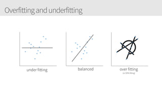
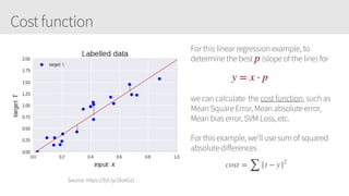
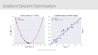
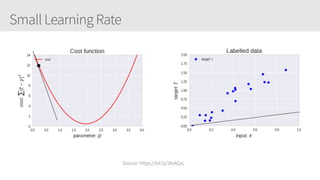
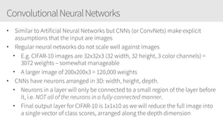
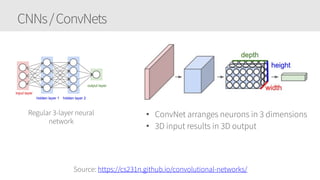
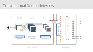
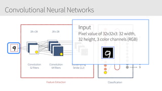
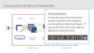
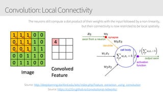
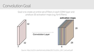
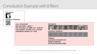
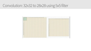
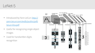
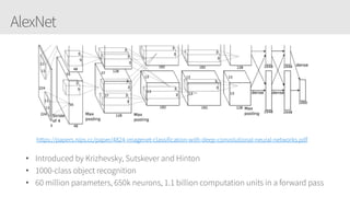
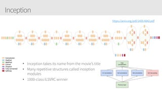
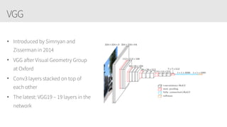
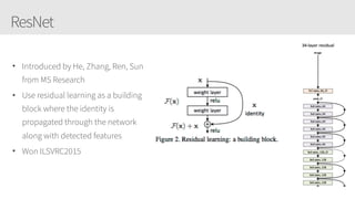
The document provides an overview of applying convolutional neural networks (CNNs), highlighting key topics such as CNN architectures, hyperparameters, cost functions, and backpropagation. It emphasizes the significance of unifying data science, engineering, and business with tools like Keras and Spark, while also featuring notable networks such as AlexNet and ResNet. Furthermore, it includes practical insights on optimizing learning rates and applying convolutions effectively in deep learning tasks.

1. Applying your
Convolutional Neural Networks

2. Logistics
• We can’t hear you…
• Recording will be available…
• Slides will be available…
• Code samples and notebooks will be available…
• Queue up Questions…

3. Accelerate innovation by unifying data science, engineering
and business
• Founded by the original creators of Apache Spark
• Contributes 75% of the open source code, 10x more than
any other company
• Trained 100k+ Spark users on the Databricks platform
VISION
WHO WE ARE
Unified Analytics Platform powered by Apache Spark™PRODUCT

4. Aboutourspeaker
Denny Lee
Technical Product Marketing Manager
Former:
• Senior Director of Data Sciences Engineering at SAP Concur
• Principal Program Manager at Microsoft
• Azure Cosmos DB Engineering Spark and Graph Initiatives
• Isotope Incubation Team (currently known as HDInsight)
• Bing’s Audience Insights Team
• Yahoo!’s 24TB Analysis Services cube

5. DeepLearningFundamentalsSeries
This is a three-part series:
• Introduction to Neural Networks
• Training Neural Networks
• Applying your Convolutional Neural Network
This series will be make use of Keras (TensorFlow backend) but as it is a
fundamentals series, we are focusing primarily on the concepts.

6. CurrentSession:ApplyingNeuralNetworks
• Diving further into CNNs
• CNN Architectures
• Convolutions at Work!

7. A quick review

8. Overfittingandunderfitting

9. Cost function
Source: https://bit.ly/2IoAGzL
For this linear regression example, to
determine the best (slope of the line) for
we can calculate the cost function, such as
Mean Square Error, Mean absolute error,
Mean bias error, SVM Loss, etc.
For this example, we’ll use sum of squared
absolute differences
y = x ⋅ p
p
cost =
∑
|t − y|2

10. Gradient Descent Optimization
Source: https://bit.ly/2IoAGzL

11. Small Learning Rate
Source: https://bit.ly/2IoAGzL

12. Small Learning Rate
Source: https://bit.ly/2IoAGzL

13. Small Learning Rate
Source: https://bit.ly/2IoAGzL

14. Small Learning Rate
Source: https://bit.ly/2IoAGzL

15. Hyperparameters:ActivationFunctions?
• Good starting point: ReLU
• Note many neural networks samples: Keras MNIST, TensorFlow CIFAR10 Pruning, etc.
• Note that each activation function has its own strengths and weaknesses. A good quote
on activation functions from CS231N summarizes the choice well:
“What neuron type should I use?” Use the ReLU non-linearity, be careful with your learning rates
and possibly monitor the fraction of “dead” units in a network. If this concerns you, give Leaky
ReLU or Maxout a try. Never use sigmoid. Try tanh, but expect it to work worse than ReLU/
Maxout.

16. SimplifiedTwo-LayerANN
Input Hidden Output
x1 → Apres Ski′er
x2 → Shredder
h1 → weather
h2 → powder
h3 → driving
Do I snowboard this weekend?

17. SimplifiedTwo-LayerANN
1
1
0.8
0.2
0.7
0.6
0.9
0.1
0.8
0.75
0.69
h1 = 𝜎(1𝑥0.8 + 1𝑥0.6) = 0.80
h2 = 𝜎(1𝑥0.2 + 1𝑥0.9) = 0.75
h3 = 𝜎(1𝑥0.7 + 1𝑥0.1) = 0.69

18. SimplifiedTwo-LayerANN
1
1
0.8
0.2
0.7
0.6
0.9
0.1
0.8
0.75
0.69
0.2
0.8
0.5
0.75
𝑜𝑢𝑡 = 𝜎(0.2𝑥0.8 + 0.8𝑥0.75 + 0.5𝑥0.69)
= 𝜎(1.105)
= 0.75

19. Backpropagation
Input Hidden Output
0.8
0.2
0.75

20. Backpropagation
Input Hidden Output
0.85
• Backpropagation: calculate the
gradient of the cost function in a
neural network
• Used by gradient descent optimization
algorithm to adjust weight of neurons
• Also known as backward propagation
of errors as the error is calculated and
distributed back through the network
of layers
0.10

21. Sigmoidfunction(continued)
Output is not zero-centered: During gradient
descent, if all values are positive then during
backpropagation the weights will become all
positive or all negative creating zig zagging
dynamics.
Source: https://bit.ly/2IoAGzL

22. LearningRateCallouts
• Too small, it may take too long to get minima
• Too large, it may skip the minima altogether

23. WhichOptimizer?
“In practice Adam is currently recommended as
the default algorithm to use, and often works
slightly better than RMSProp. However, it is often
also worth trying SGD+Nesterov Momentum as
an alternative..”
Andrej Karpathy, et al, CS231n
Source: https://goo.gl/2da4WY
Comparison of Adam to Other Optimization Algorithms Training a Multilayer Perceptron
Taken from Adam: A Method for Stochastic Optimization, 2015.

24. Optimizationonlosssurfacecontours
Adaptive algorithms converge
quickly and find the right direction
for the parameters.
In comparison, SGD is slow
Momentum-based methods
overshoot
Source: http://cs231n.github.io/neural-networks-3/#hyper
Image credit: Alec Radford

25. Optimizationonsaddlepoint
Notice how SGD gets stuck near the
top
Meanwhile adaptive techniques
optimize the fastest
Source: http://cs231n.github.io/neural-networks-3/#hyper
Image credit: Alec Radford

26. GoodReferences
• Suki Lau's Learning Rate Schedules and Adaptive Learning Rate Methods for
Deep Learning
• CS23n Convolutional Neural Networks for Visual Recognition
• Fundamentals of Deep Learning
• ADADELTA: An Adaptive Learning Rate Method
• Gentle Introduction to the Adam Optimization Algorithm for Deep Learning

27. Convolutional Networks

28. ConvolutionalNeuralNetworks
• Similar to Artificial Neural Networks but CNNs (or ConvNets) make explicit
assumptions that the input are images
• Regular neural networks do not scale well against images
• E.g. CIFAR-10 images are 32x32x3 (32 width, 32 height, 3 color channels) =
3072 weights – somewhat manageable
• A larger image of 200x200x3 = 120,000 weights
• CNNs have neurons arranged in 3D: width, height, depth.
• Neurons in a layer will only be connected to a small region of the layer before
it, i.e. NOT all of the neurons in a fully-connected manner.
• Final output layer for CIFAR-10 is 1x1x10 as we will reduce the full image into
a single vector of class scores, arranged along the depth dimension

29. CNNs/ConvNets
Regular 3-layer neural
network
• ConvNet arranges neurons in 3 dimensions
• 3D input results in 3D output
Source: https://cs231n.github.io/convolutional-networks/

30. Convolutional Neural Networks
28 x 28 28 x 28 14 x 14
Convolution
32 filters
Convolution
64 filters
Subsampling
Stride (2,2)
Feature Extraction Classification
0
1
8
9
FullyConnected
Dropout
Dropout

31. Convolutional Neural Networks
28 x 28 28 x 28 14 x 14
Convolution
32 filters
Convolution
64 filters
Subsampling
Stride (2,2)
Feature Extraction Classification
0
1
8
9
FullyConnected
Dropout
Dropout
Input
Pixel value of 32x32x3: 32 width,
32 height, 3 color channels (RGB)

32. Convolutional Neural Networks
28 x 28 28 x 28 14 x 14
Convolution
32 filters
Convolution
64 filters
Subsampling
Stride (2,2)
Feature Extraction Classification
0
1
8
9
FullyConnected
Dropout
Dropout
Convolutions
Compute output of neurons (dot
product between their weights)
connected to a small local region. If
we use 32 filters, then the output is
28x28x32 (using 5x5 filter)

33. Convolution:Kernel=Filter
During forward pass, we
slide over the image spatially
(i.e. convolve) each filter
across the width and height,
computing dot products.
Source: http://deeplearning.stanford.edu/wiki/index.php/Feature_extraction_using_convolution
kernel = filter = feature detector

34. Convolution:LocalConnectivity
Connect neurons to only a
small local region as it is
impractical to connect to all
neurons. Depth of filter =
depth of input volume.
Source: http://deeplearning.stanford.edu/wiki/index.php/Feature_extraction_using_convolution

35. Convolution:LocalConnectivity
Source: http://deeplearning.stanford.edu/wiki/index.php/Feature_extraction_using_convolution
Source: https://cs231n.github.io/convolutional-networks/
The neurons still compute a dot product of their weights with the input followed by a non-linearity,
but their connectivity is now restricted to be local spatially.

36. ConvolutionGoal
Goal is to create an entire set of filters in each CONV layer and
produce 2D activation maps (e.g. for 6 filters)
Source: http://cs231n.stanford.edu/slides/2017/cs231n_2017_lecture5.pdf

37. ConvolutionExamplewith8filters
Source: https://cs.stanford.edu/people/karpathy/convnetjs/demo/mnist.html

38. Convolution:32x32to28x28using5x5filter

39. Takingastride…
Stride = 1 Stride = 2
Stride = 3
Does not fit!
Output Size:
(N – F) / stride + 1
e.g. N = 7, F = 3:
Stride 1 = 5
Stride 2 = 3
Stride 3 = 2.33 (doh!)
Source: http://cs231n.stanford.edu/slides/2017/cs231n_2017_lecture5.pdf

40. Padding
0 0 0 0
0
0
0
0
Source: http://cs231n.stanford.edu/slides/2017/cs231n_2017_lecture5.pdf
Zero pad image border to preserve size spatially
Input: 7 x 7
Filter: 3 x 3
Stride = 1
Zero Pad = 1
Output: 7 x 7
0 0 0 0 0 0
0 0 0 0 0 0
0 0
0 0
0 0
0 0
Input: 7 x 7
Filter:5 x 5
Stride = 1
Zero Pad = 2
Output: 7 x 7
Common Practice:
• Stride = 1
• Filter size: F x F
• Zero Padding: (F – 1)/2

41. CalculateOutputSize
1 2 3 4 5 6 7 8 9 10 11 12 13 14 15 16 17 18 19 20 21 22 23 24 25 26 27 28 29 30 31 32
2
3
4
5
6
7
8
9
10
11
12
13
14
15
16
17
18
19
20
21
22
23
24
25
26
27
28
29
30
31
32
Input: 32 x 32 x 3
5 5x5 filters
Stride = 1
Padding = 2
Output Volume Size:
Source: http://cs231n.stanford.edu/slides/2017/
cs231n_2017_lecture5.pdf
(Input + 2) x Padding − Filter
Stride + 1
=
(32 + 2) x 2 − 5
1 + 1
= 32
32 x 32 x 5

42. 5 5x5 filters
CalculateOutputSize
1 2 3 4 5 6 7 8 9 10 11 12 13 14 15 16 17 18 19 20 21 22 23 24 25 26 27 28 29 30 31 32
2
3
4
5
6
7
8
9
10
11
12
13
14
15
16
17
18
19
20
21
22
23
24
25
26
27
28
29
30
31
32
Input: 32 x 32 x 3
Stride = 1
Padding = 2
Number of Parameters
Source: http://cs231n.stanford.edu/slides/2017/
cs231n_2017_lecture5.pdf
(Filter x Filter x Depth + 1)(# of Filters) =
(5 x 5 x 3 + 1) x (5) =
380

43. Convolutional Neural Networks
28 x 28 28 x 28 14 x 14
Convolution
32 filters
Convolution
64 filters
Subsampling
Stride (2,2)
Feature Extraction Classification
0
1
8
9
FullyConnected
Dropout
Dropout
Activation Function (ReLU)
Compute output of neurons (dot
product between their weights)
connected to a small local region. If
we use 32 filters, then the output is
28x28x32 (using 5x5 filter)

44. ReLUStep(LocalConnectivity)
Source: http://deeplearning.stanford.edu/wiki/index.php/Feature_extraction_using_convolution
Source: https://cs231n.github.io/convolutional-networks/
The neurons still compute a dot product of their weights with the input followed by a non-linearity,
but their connectivity is now restricted to be local spatially.

45. Convolutional Neural Networks
28 x 28 28 x 28 14 x 14
Convolution
32 filters
Convolution
64 filters
Subsampling
Stride (2,2)
Feature Extraction Classification
0
1
8
9
FullyConnected
Dropout
Dropout
Pooling
Perform down sampling operation
along spatial dimensions (w, h)
resulting in reduced volume,
e.g. 14x14x2.

46. Pooling=subsampling=reduceimagesize
Source: https://cs231n.github.io/convolutional-networks/#pool
• Commonly insert pooling
layers between
successive convolution
layers
• Reduces size spatially
• Reduces amount of
parameters
• Minimizes likelihood of
overfitting

47. Poolingcommonpractices
Source: https://cs231n.github.io/convolutional-networks/#pool
• Input:
• Output:
• Typically or
. (overlap pooling)
• Pooling with larger receptive fields
(. ) too destructive.
{𝐹 = 2, 𝑆 = 2}
W1 x H1 x D1
W2 x H2 x D2 where
W2 =
(W1 − F)
S
+ 1, D2 = D1
H2 =
(H1 − F)
S
+ 1
{F = 2, S = 2}
{F = 3, S = 2}
{F}

48. Stride,Pooling,Ohmy!
• Smaller strides = Larger Output
• Larger strides = Smaller Output (less overlaps)
• Less memory required (i.e. smaller volume)
• Minimizes overfitting
• Potentially use larger strides in convolution layer to reduce
number of pooling layers
• Larger strides = smaller output reduce in spatial size ala pooling
• ImageNet 2015 winner ResNet has only two pooling layers

49. Convolutional Neural Networks
28 x 28 28 x 28 14 x 14
Convolution
32 filters
Convolution
64 filters
Subsampling
Stride (2,2)
Feature Extraction Classification
0
1
8
9
FullyConnected
Dropout
Dropout
Fully Connected
Neurons in a fully connected layer
have full connections to all
activations in the previous layer, as
seen in regular Neural Networks.

50. Convolutional Neural Networks Layers
28 x 28 28 x 28 14 x 14
Convolution
32 filters
Convolution
64 filters
Subsampling
Stride (2,2)
Feature Extraction Classification
0
1
8
9
FullyConnected
Dropout
Dropout

51. https://cs.stanford.edu/people/karpathy/convnetjs/demo/mnist.html
ConvNetJS MNIST Demo

52. CNN Architectures

53. LeNet-5
• Introduced by Yann LeCun: http://
yann.lecun.com/exdb/publis/pdf/
lecun-01a.pdf
• Useful for recognizing single object
images
• Used for handwritten digits
recognition

54. AlexNet
• Introduced by Krizhevsky, Sutskever and Hinton
• 1000-class object recognition
• 60 million parameters, 650k neurons, 1.1 billion computation units in a forward pass
https://papers.nips.cc/paper/4824-imagenet-classification-with-deep-convolutional-neural-networks.pdf

55. Inception
https://arxiv.org/pdf/1409.4842.pdf
• Inception takes its name from the movie’s title
• Many repetitive structures called inception
modules
• 1000-class ILSVRC winner

56. VGG
• Introduced by Simnyan and
Zisserman in 2014
• VGG after Visual Geometry Group
at Oxford
• Conv3 layers stacked on top of
each other
• The latest: VGG19 – 19 layers in the
network

57. ResNet
• Introduced by He, Zhang, Ren, Sun
from MS Research
• Use residual learning as a building
block where the identity is
propagated through the network
along with detected features
• Won ILSVRC2015

58. Neurons … Activate!
DEMO

59. I’d like to thank…

60. GreatReferences
• Andrej Karparthy’s ConvNetJS MNIST Demo
• What is back propagation in neural networks?
• CS231n: Convolutional Neural Networks for Visual Recognition
• Syllabus and Slides | Course Notes | YouTube
• With particular focus on CS231n: Lecture 7: Convolution Neural Networks
• Neural Networks and Deep Learning
• TensorFlow

61. GreatReferences
• Deep Visualization Toolbox
• Back Propagation with TensorFlow
• TensorFrames: Google TensorFlow with Apache Spark
• Integrating deep learning libraries with Apache Spark
• Build, Scale, and Deploy Deep Learning Pipelines with Ease

62. Attribution
Tomek Drabas
Brooke Wenig
Timothee Hunter
Cyrielle Simeone

63. Q&A

64. What’s next?
State Of The Art Deep Learning On Apache Spark™
October 31, 2018 | 09:00 PDT
https://dbricks.co/2NqogIp