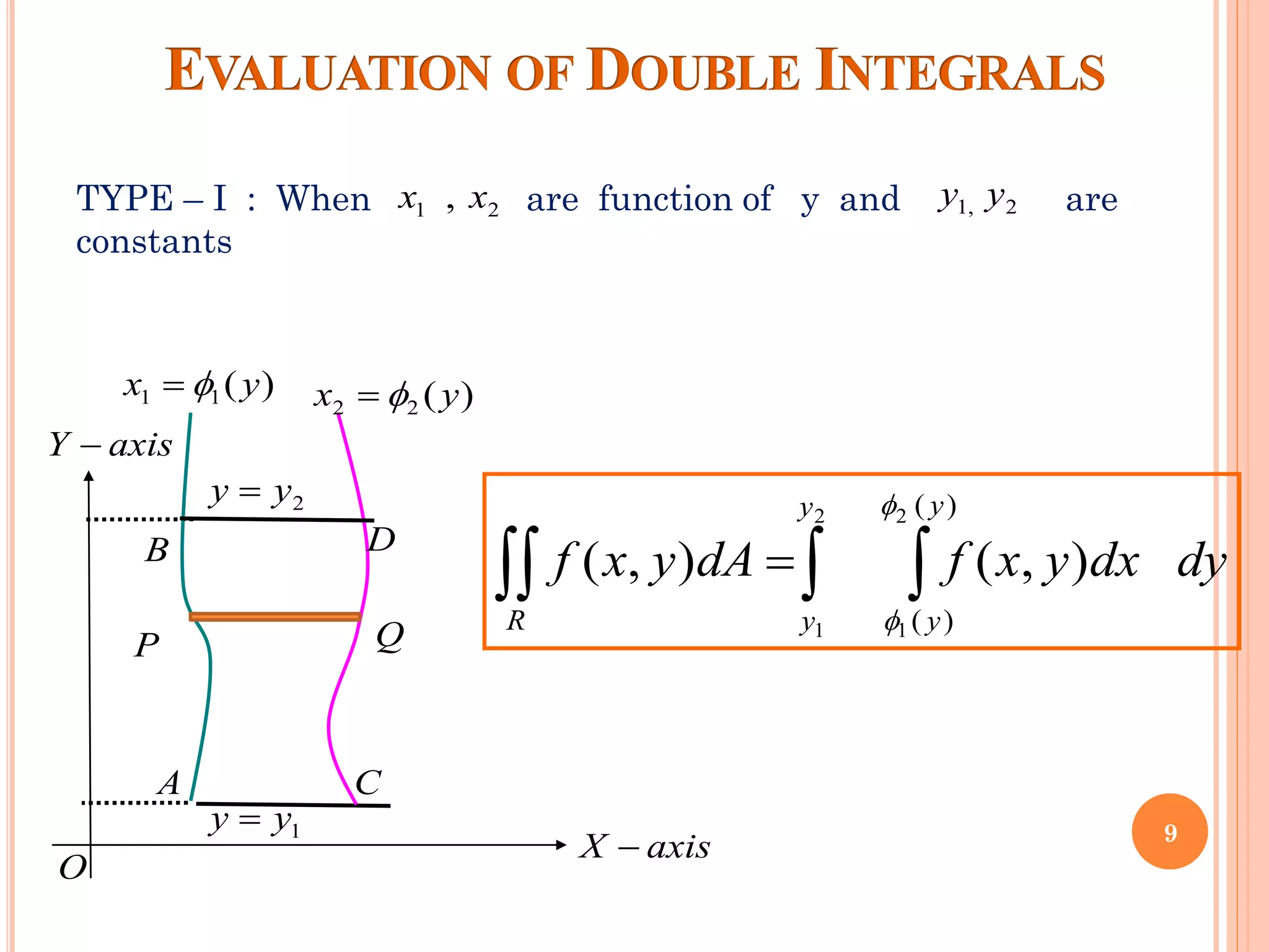
1
By
Mrs. Geetanjali P. Kale
Guru Nanak Institute of Technology,
Nagpur
Contain :
❑ Introduction
❑ Double Integrals in Cartesian
Coordinates
❑ Double Integrals in Polar Coordinates
❑ Change of Order of Integration
❑ Triple Integration
❑ Application
2
Why to study Multiple Integral ?
▪ To find the area of the region bounded by
curves ,we require double integrals.
▪ To find the volume of a solid , we require triple
integrals.
▪ To find the surface area of the solid obtained
by revolving the curve.
3
▪ To find mass , Center of gravity , Center of
Pressure , Moment of Inertia we require
Multiple integral.
▪In vector calculus we have the relationship
between these multiple integrals (Green’s
Theorem , Stoke’s Theorem and Gauss
Divergence Theorem) which have
applications in the subject E.M.F. of
Engineering field.
▪ Multiple Integrals are very much required
to understand many concepts of Engineering
and Technology.
4
The definite integral is defined as the
limit of the sum

b
a
dx
x
f )
(
n
n x
x
f
x
x
f
x
x
f 

 )
(
.
..........
)
(
)
( 2
2
1
1 +
+
+
When and each of the lengths
tends to zero . Here are n sub-
intervals into which the range b - a has been
divided and are values of x lying
respectively in the first , second , . . . . . . . ., nth
subinterval .

→
n
n
x
x
x
x 


 ,........,
,
, 3
2
1
n
x
x
x
x ,........,
,
, 3
2
1
5
Our goal is to find the volume of S.
}
)
,
(
),
,
(
0
)
,
,
{( 3
R
y
x
y
x
f
z
R
z
y
x
s 



=
6
7
8
TYPE – I : When are function of y and are
constants
2
1 , x
x 2
,
1 y
y
A
Q
P
C
D
B
O
axis
Y −
axis
X −
)
(
2
2 y
x 
=
)
(
1
1 y
x 
=
2
y
y =
1
y
y =
 
 =
2
1
2
1
)
(
)
(
)
,
(
)
,
(
y
y
y
y
R
dy
dx
y
x
f
dA
y
x
f


9
TYPE – I : When are function of x and are
constants
2
1 , y
y 2
,
1 x
x
Y-axis
X – axis
A
Q
C
D
B
O
)
(
2
2 x
y 
=
)
(
1
1 x
y 
=
2
x
x =
1
x
x =
 
 =
2
1
2
1
)
(
)
(
)
,
(
)
,
(
y
y
x
x
R
dy
dx
y
x
f
dA
y
x
f


10
TYPE – I : When are constants
2
1
2
,
1 ,
, y
y
x
x
R
axis
Y −
axis
X −
2
x
x =
1
x
x =
2
y
y =
1
y
y =
 
   =
=
2
1
2
1
2
1
2
1
)
,
(
)
,
(
)
,
(
then
R
y
y
x
x
x
x
y
y
dy
dx
y
x
f
dx
dy
y
x
f
dA
y
x
f
11
Evaluate the following
integral
 
−
+
2
1
1
1
2
)
2
3
(
(i) dx
dy
xy
x
12
 
 
 
14
)
1
(
2
)
2
(
2
2
6
]
)
1
(
)
1
(
3
[
]
)
1
(
)
1
(
3
[
3
)
2
3
(
)
2
3
(
have
we
,
constants
are
n
integratio
of
limits
the
Since
3
3
2
1
3
2
1
2
2
1
2
2
2
2
2
1
1
1
2
2
2
1
1
1
2
2
1
1
1
2
=
−
=
=
=
−
+
−
−
+
=
+
=








+
=
+



 
 
=
−
=
=
=
=
−
=
−
x
dx
x
dx
x
x
x
x
dx
xy
y
x
dx
dy
xy
x
dydx
xy
x
y
y
x
x
y
y
13
 
2
0
,
2
:
)
,
(
;
4
)
,
(
where
)
,
(
Evaluate
2




=
−
=

y
y
x
y
y
x
R
y
x
y
x
f
dy
dx
y
x
f
R
x
y
2
=
y
0
=
y
y
x 2
=
2
y
x =
as
d
illustrate
is
R
region
The
(i)
14
 
5
36
5
2
4
2
)
2
6
(
]}
)
(
2
[
]
2
)
2
(
2
{[
2
)
4
(
)
4
(
2
0
5
4
3
2
0
4
3
2
2
0
3
2
2
2
2
2
0
2
2
2
0
2
2
2
=






−
+
=
−
+
=
−
−
−
=
−
=
−
=
−



 

=
=
=
=
=
=
y
y
y
dy
y
y
y
dy
y
y
y
y
dy
xy
x
dxdy
y
x
dxdy
y
x
y
x
y
x
y
y
y
x
y
x
R
15
x
y
y
x
x
R
y
y
x
f
dy
dx
y
x
f
R
sin
and
0
,
,
0
bounded
region
the
is
;
)
,
(
)
,
(
Evaluate
(ii)
=
=
=
=
=


x
y
x
y sin
=
0
=
y
0
=
x 
=
x
as
d
illustrate
is
R
region
The
16
4
2
2
sin
4
1
)
2
cos
1
(
4
1
2
sin
2
)
,
(
0
0
0
2
0
sin
0
2
0
sin
0






=






−
=
−
=
=






=
=



 

=
=
=
=
x
x
dx
x
dx
x
dx
y
dydx
y
dxdy
y
x
f
x
x
x
x
y
y
R
17
 
 
2
0
1
2
2
(ii)
0
sin
(i)
Evaluate
y
dxdy
x
e
x
dydx
y
y

(i) The Region of Integration R is :
y : x to
x : 0 to
x

=
y

=
x
y
0
=
x
x
y =
R
18

 
+
+
−
1
0 0
2
2
2
2
0
4
0
2
2
)
(
(ii)
)
cos(
(i)
s
coordinate
polar
to
changing
by
integrals
following
the
Evaluate
2
y
x
dxdy
y
x
y
dydx
y
x
19
as
described
is
R
n
integratio
of
region
The
(i)
2
4 x
y −
=
0
=
y
0
=
x 2
=
x
2
0
2
2
−
X
Y
20
 
4
4
sin
4
sin
sin
)
(cos
)
(cos
)
cos(
Therefore
2
/
0
2
1
2
/
0
4
0
2
1
2
/
0
4
0
2
1
2
/
0
2
0
2
2
0
4
0
2
2
2









=
=
=
=
=
+


 
 
 
−
d
d
u
dud
u
rdrd
r
dydx
y
x
x
0
=
r
2
=
r
0
=

2
/

 =
21
as
described
is
R
n
integratio
of
region
The
(ii)
0
=
y
0
=
x
axis
Y −
y
x =
1
=
y
R
axis
X −
22
8
4
2
2
1
2
1
cos
2
sec
cos
2
cos
)
cos
(
Therefore
2
/
4
/
2
/
4
/
2
2
2
/
4
/
2
sec
0
2
2
/
4
/
sec
0
2
2
/
4
/
sec
0
2
2
1
0 0
2
2
2


























=






−
=
=
=






=
=








=








+



 
 

=
=
d
d
d
r
drd
r
rdrd
r
r
dxdy
y
x
y
r
r
y
4
/

 =
y

sec
=
r
x
2
/

 =
23

R
dA
y
x
f )
,
(
Evaluate
(-2,1)
and
(3,1)
(0,0),
vertices
h the
region wit
r
triangula
closed
the
is
;
)
,
(
, 2
R
xy
y
x
f
where =
(i) The Region of Integration R is
illustrated below :
0
=
y
y
x 2
−
=
X
1
=
y
y
x 3
=
1
2
− 3
R
Y
)
0
,
0
(
)
1
,
2
(− )
1
,
3
(
24
   
=
=
=
=
=
= 

















=
=
=
=
=
=
=
b
z
a
z
(z)
y
(z)
y
)
z
,
(y
f
x
)
z
,
y
(
f
x
2
1
2
2
1
1
2
2
1
1
2
1
2
2
1
1
2
2
1
1
dx
)
z
,
y
,
x
(
f
)
z
,
y
x,
f(
followes
as
evaluated
is
integral
triple
then the
,
b
z
,
a
z
and
(z)
y
,
(z)
y
,
)
z
,
(y
f
x
,
)
z
,
y
(
f
x
Let
dz
dy




25
  
−
1
0
1 1
0
2
6
x
y
dz
dy
dx
z
Evaluate
dx
dy
dz
z
dz
dy
dx
z
x x
y
y
z
x
y
  
   = =
−
=
−


















=
1
0
1 1
0
1
0
1 1
0 2
2
6
6
dx
dy
y
dx
dy
z
x x
y
x x
y
y
z
z
 
 
= =
= =
−
=
=








−
=














=
1
0
1
2
1
0
1 1
0
2
2
2
)
1
(
3
2
6
26
dx
x
dx
y
x
x
x
3
2
1
0
1
1
0
3
)
1
(
3
)
1
(
3
2
−
=






−
−
=


=
=
35
16
7
5
3
)
3
3
1
(
1
0
7
5
3
1
0
6
4
2
=






−
+
−
=
−
+
−
= 
x
x
x
x
dx
x
x
x
27
Area by Double
Integration
a) Cartesian Co-ordinates : The area A of the region
bounded by the curves and the
lines x = a , x= b is given by ,
)
(
,
)
( 2
1 x
f
y
x
f
y =
=
 
=
b
a
x
f
x
f
dx
dy
A
)
(
)
(
2
1
The area A of the region bounded by the curves
and the lines y = c , y = d is
given by,
)
(
,
)
( 2
1 y
f
x
y
f
x =
=
 
=
d
c
y
f
y
f
dy
dx
A
)
(
)
(
2
1
28
b) Polar Co-ordinates :
The area of region bounded by the curve
and the lines is given by ,
 
=





)
(
)
(
2
1
f
f
d
dr
r
A
)
(
,
)
( 2
1 
 f
r
f
r =
=



 =
= ,
29
Find the smaller of the areas bounded by
the ellipse and the
straight line
36
9
4 2
2
=
+ y
x
6
3
2 =
+ y
x
1
4
9
2
2
=
+
y
x
The equation of the ellipse is
And the line is
1
2
3
=
+
y
x
The point of intersection of both curves are
A(3 , 0 ) and B(0 , 2)
30
R
A(3 , 0 )
B(0,2)
Y-axis
X-axis
2
4
2
3
y
x −
=
)
2
(
2
3
y
x −
=
(0 , 0 )
From figure we have :
2
4
2
3
)
2
(
2
3
: y
to
y
x −
−
Q
P
2
0
: to
y
31
Thus the required area is :
 
=
−
−
=
=
2
0
4
2
3
)
2
(
2
3
2
y
y
y
x
dy
dx
A
 
2
0
2
1
2
2
2
0
4
2
3
)
2
(
2
3
2
0
2
2
2
sin
2
4
2
4
2
3
)
2
(
2
3
4
2
3
2








+
−
+
−
=






−
−
−
=
=
−
=
−
−
=


y
y
y
y
y
dy
y
y
dy
x
y
y
y
y
32
 
( )
2
2
3
2
2
2
2
3
2
4
1
sin
2
2
3 1
−
=







−
•
=
+
−
= −


A
33
34
The total electric charge
on a solid object occupying a region E
and having charge density σ(x, y, z) is:
( )
, ,
E
Q x y z dV

= 
TOTAL ELECTRIC CHARGE
35
Find the center of mass of a solid of constant density that
is bounded by the parabolic cylinder x = y2 and the planes x
= z, z = 0,
and x = 1.
Example 5
APPLICATIONS
36
The solid E and its projection onto
the xy-plane are shown.
Example 5
APPLICATIONS
Fig. 16.6.14a, p. 1033 Fig. 16.6.14b, p. 1033
37
The lower and upper
surfaces of E are
the planes
z = 0 and z = x.
 So, we describe E
as a type 1 region:
( )
 
2
, , 1 1, 1,0
E x y z y y x z x
= −      
Example 5
APPLICATIONS
Fig. 16.6.14a, p. 1033
38
Then, if the density is ρ(x, y, z),
the mass is:
Example 5
APPLICATIONS
2
2
1 1
1 0
1 1
1
E
x
y
y
m
dV
dz dxdy
xdxdy



−
−
=
=
=

  
 
39
APPLICATIONS
( )
( )
2
1
2
1
1
1
4
1
1
4
0
1
5
0
2
1
2
1
4
5 5
x
x y
x
dy
y dy
y dy
y
y





=
−
=
−
 
=  
 
= −
= −
 
= − =
 
 



Example 5
40
Due to the symmetry of E and ρ about
the xz-plane, we can immediately say that
Mxz = 0, and therefore .
The other moments are calculated
as follows.
0
y =
Example 5
APPLICATIONS
41
2
2
1 1
1 0
1 1
2
1
yz
E
x
y
y
M
x dV
x dz dxdy
x dxdy



−
−
=
=
=

  
 
Example 5
APPLICATIONS
42
APPLICATIONS
( )
2
1
3
1
1
1
6
0
1
7
0
3
2
1
3
2
3 7
4
7
x
x y
x
dy
y dy
y
y




=
−
=
 
=  
 
= −
 
= −
 
 
=


Example 5
43
( )
2
2
2
1 1
1 0
2
1 1
1
0
1 1
2
1
1
6
0
2
2
2
1
3 7
x
xy y
E
z x
y
z
y
M z dV z dz dxdy
z
dxdy
x dxdy
y dy
 


 
−
=
−
=
−
= =
 
=  
 
=
= − =
   
 
 

Example 5
APPLICATIONS
44
Therefore, the center of mass is:
( )
( )
5 5
7 14
, , , ,
,0,
yz xy
xz
M M
M
x y z
m m m
 
=  
 
=
Example 5
APPLICATIONS
45

Applied Mathematics Multiple Integration by Mrs. Geetanjali P.Kale.pdf