Analysis on flat plate and beam supported slab

1
CERTIFICATE
This is to certify that the project report entitled “Finite Element Analysis of Flat Plate & Beam
Supported Slab” for the award of the degree of B.sc in civil engineering, is a bona fide record
of the research work done by them under my supervision. The project has not been submitted
earlier either to this university or elsewhere for the fulfillment of the requirement of any
course.
MD. TARIKUL ISLAM
SUPERVISOR, PROJECT AND THESIS
SR. LECTURER AND COURSE COORDINATOR
DEPARTMENT OF CIVIL ENGINEERING.
UNIVERSITY OF INFORMATION TECHNOLOGY AND SCIENCES

2
DECLARATION
We declare that this dissertation has not been previously accepted in substance
for any degree and is not being submitted in candidature for any degree. We
state that this dissertation is the result of our own independent
work/investigation, except where otherwise stated.
We hereby give consent for any dissertation, if accepted, to be available for
photocopying and understand that any reference to or quotation from my thesis
will receive an acknowledgement.
Md. Imran Hossain
ID: 12310177
Md. Ruhul Amin
ID: 12410196
Md. Dider-E-Alam
ID: 11510086
Md. Tarikul Islam

3
Course Code: CE 490
Course Title: Project
Project On
Finite Element Analysis of Flat Plate & Beam Supported
Slab
Written by
Md. Imran Hossain(12310177)
Student,Dept. of Civil Engineering, UITS
Md. Ruhul Amin (12410196)
Md. Dider-E-Alam (11510086)

4
To the memory of our honorable teacher
Md. Tarikul Islam
Lecturer, Dept. of Civil Engineering, UITS
Submission Date:

5
Acknowledgement
At first all praises belong to the Almighty, the most Merciful, the most
Beneficent to men and His action, which provides us the chance to conduct this
study.
We express our gratitude to Md. Tarikul Islam, lecturer, department of
civil Engineering, UITS for his guidance, advice and encouragement towards the
successful completion of the study.
We express our thanks to the fellow students of Department of Civil Engineering
for their active help and advice.
Finally, I like to thank all of them who wished my well and inspired us for the
completion of the study.

6
Table of Contents
Chapter 1 Introduction
1.1 General ………………………………………………………………………………………………13
1.2 Slab System ………………………………………………………………………………………..14
1.3 Objective of the Study ……………………………………………………………………….15
Chapter 2 Literature Review
2.1 General ………………………………………………………………………………………………16
2.2 Classification of Slab……………………………………………………………………………17
2.3 Concrete slab floors…………………………………………………………………………….17
2.4 Different types…………….…………………………………………………….……………..…17
2.4.1 Slab on grounds…..……………………………………………………………………………17
2.4.2 Suspended Slab.....................................................................................18
2.4.3 Precast slab…….....................................................................................18
2.5 Types of Slab…………………………….………………….………………………………………18
2.6 Load path/Framing possibilities of Slab………..………………………………………21
2.6.1Two load path options……………………………………………………………………….22
2.7 Behavior of one way slab…………..…………………………………………………………23
2.8 Behavior of two slab…..………………..………………………………………………………24
2.9 One way Slabs…….....................................................................................24
2.10 Two way Slabs……..................................................................................29
2.10.1 Two way column Supported slab (Flat plate)……….………………….........29
2.11 Slab analysis method……………................................................................33
2.11.1 Direct design method…….…................................................................33
2.11.2 Equivalent frame method…................................................................34
2.11.3 Finite element method………………………...............................................35
2.11.3.1 Introduction..................…................................................................35

7
2.11.3.2 What is FE and why use it? ...............................................................35
2.11.3.3 History...........................…................................................................36
2.11.3.4 When to FE analysis………………………................................................36
2.11.3.5 Advantages……………………................................................................37
2.11.3.6 Disadvantages……………………………….................................................37
2.11.3.7 Finite Element Software…………………...............................................37
2.11.4 Staad.Pro……………….…………................................................................38
2.11.4.1 Introduction……………………...............................................................38
2.11.4.2 About Staad Pro……….……................................................................39
2.11.4.3. Features of Staad Pro……………………….............................................40
2.11.4.4 Techniques for slab design using FEA by Staad.Pro….......................41
2.11.4.4.1 Design using average stress resultants…………….…….....................42
2.11.4.4.2 Computation of design moments using bending moment...........47
2.11.4.5 Design……………………………………….....................................................48
2.11.4.6 Conclusion……………….……................................................................49
Chapter 3 Design Methodology
3.1 General ………………………………………………………………………………………………50
3.2 Plan of Flat plate & Beam supported slab……………………………………………51
3.3 Flat Plate design…….……………………………………………………………………………52
3.4 Basic data for the Structures……………………………………………………………….52
3.5 Design Procedure by Staad.pro…………………………………………………………...52
3.6 Analysis of a plate...............................................................................…...64
3.7 Viewing the output file for flat plate .................................................…...65
3.8 Post processing…………………………………………………………………………………...65
3.9 Staad pro. Output file for beam supported slab……………………………….…...74

8
Chapter 4 Results & Discussions
4.1 General ……………………………………………………………………………….………………75
4.2 Mesh analysis…..…….……………………………………………………………………………76
4.2.1 Summary of Flat Plat & Beam Supported Slab (25x25 Mesh)…………….76
4.2.2 Summary of Flat Plat & Beam Supported Slab (50x50 Mesh)……………..79
4.3 Stress Analysis....................................................................................…...82
4.3.1 Summary of Stress for Flat Plat & Beam Supported Slab................…...82
4.4 Displacement analysis........................................................................…...85
4.4.1 Summary of displacement for Flat Plate & Beam Supported Slab...…...85
Chapter 5 Conclusion & Recommendation
5.1 Conclusion ….………………………………………………………………………………………98
5.2 Recommendation.….……………………………………………………………………………98

9
List of Figures
Fig. 2.1 Suspended slab............................................................................................................18
Fig. 2.2 One way slab without beam & with beam slab ..........................................................19
Fig. 2.3 Two way slab & grid slab............................................................................................19
Fig. 2.4 Flat plate slab & flat slab.............................................................................................19
Fig. 2.5 Three dimensional view of one way slab, two way slab.............................................20
Fig.2.6 Three dimensional view of flat plate and flat slab.......................................................20
Fig. 2.7 One way slab load path...............................................................................................22
Fig. 2.8 Two way slab load path...............................................................................................23
Fig. 2.9 Behavior of one way slab ............................................................................................23
Fig. 2.10 Behavior of two way slab ..........................................................................................24
Fig. 2.11 Flat plate short & long direction ...............................................................................30
Fig. 2.12 Effective beam of flat plate.......................................................................................30
Fig. 2.13 Critical moment section ............................................................................................31
Fig. 2.14 Moment variation along a span ................................................................................32
Fig. 2.15 Moment variation across the width of critical section .............................................32
Fig. 2.16 portion of the slab to include with beam.................................................................33
Fig. 2.17 Element stress resultants at a node..........................................................................43
Fig. 2.18 X-direction strip selection based on Mxx contour plan ............................................46
Fig. 2.19 Average Bending Moment Resultants at each node along cut.................................48
Fig. 3.1 Plan of flat plate & beam supported slab ...................................................................51
Fig. 3.2 Starting page of Staad pro...........................................................................................52
Fig. 3.3 Selected plane in Staad pro.........................................................................................53
Fig. 3.4 Plate selected ..............................................................................................................54
Fig. 3.5 Grid settings ................................................................................................................55
Fig. 3.6 Mesh settings page......................................................................................................56
Fig. 3.7 Thickness settings........................................................................................................56
Fig. 3.8 Assign to Plate .............................................................................................................57
Fig. 3.9 Same plate thickness...................................................................................................57

10
Fig. 3.10 Support reaction........................................................................................................58
Fig. 3.11 Assigned support.......................................................................................................58
Fig. 3.12 Load case...................................................................................................................59
Fig. 3.13 Load definition...........................................................................................................59
Fig. 3.14 Self weight.................................................................................................................60
Fig. 3.15 pressure on Plate.......................................................................................................60
Fig. 3.16 Flat slab whole structure...........................................................................................61
Fig. 3.17 Load of partition wall ................................................................................................61
Fig. 3.18 Load combination......................................................................................................62
Fig. 3.19 Load combination......................................................................................................62
Fig. 3.20 Analysis......................................................................................................................63
Fig. 3.21 Analysis Structure......................................................................................................63
Fig. 3.22 Analysis/ Print............................................................................................................64
Fig. 3.23 View output file.........................................................................................................64
Fig. 3.24 Viewing stress values in a tabular form ....................................................................66
Fig. 3.25 Plate center stress table............................................................................................66
Fig. 3.26 Stress contour............................................................................................................68
Fig. 3.27 Stress contour............................................................................................................68
Fig. 3.28 Flat slab......................................................................................................................69
Fig. 3.29 Plate edge length & area...........................................................................................70
Fig. 3.30 Plate Stress ................................................................................................................70
Fig. 3.31 Plate Force.................................................................................................................71
Fig. 3.32 Plate Force ................................................................................................................71
Fig. 3.33 Plate Force tabular form ...........................................................................................72
Fig. 3.34 Moment value diagram.............................................................................................73
Fig. 3.35 Force & Moment table .............................................................................................73
Fig. 3.36 Force & Moment table .............................................................................................74
Fig. 4.1 Mesh analysis for flat plate 25*25 .............................................................................78
Fig. 4.2 Mesh analysis for beam slab 25*25 ...........................................................................78
Fig. 4.3 Mesh analysis for beam slab 50*50 ............................................................................81
Fig. 4.3 Mesh analysis forflat plate 50*50 ...............................................................................81
Fig. 4.5 Graph for Maximum Moment.....................................................................................84

11
Fig. 4.6 Displacement 25*25 & 50*50 .....................................................................................87
Fig. 4.7 Displacement beam supported slab 25*25.................................................................87
Fig. 4.8 Displacement flat plate 25*25 ....................................................................................88
Fig. 4.9 Displacement beam supported slab 50*50.................................................................88
Fig. 4.10 Displacement flat plate 50*50 ..................................................................................89
List of Tables
Table 2.1 Area of bars in slab...................................................................................................26
Table 2.2 Minimum thickness of one way slab........................................................................27
Table 2.3 Flexure resistance factor .........................................................................................28
Table 4.1 Plate center Stress Mesh(25x25) .............................................................................76
Table 4.2 Beam supported slab center Stress Mesh(25x25) ...................................................77
Table 4.3 Plate center Stress Mesh(50x50) .............................................................................79
Table 4.4 Beam supported slab center Stress Mesh(50x50) ...................................................80
Table 4.5 Center principal Stress for flat plate Mesh(25x25)..................................................82
Table 4.6 Center principal Stress for beam supported slab Mesh(25x25) ..............................82
Table 4.7 Center principal Stress for flat plate Mesh(50x50)..................................................83
Table 4.8 Center principal Stress for beam supported slab Mesh(50x50) ..............................83
Table 4.9 Node displacement for flat plate(25x25).................................................................85
Table 4.10 Node displacement for beam supported slab(25x25) ...........................................85
Table 4.11 Node displacement for flat plate(50x50)...............................................................86
Table 4.12 Node displacement for beam supported slab(50x50) ...........................................86

12
Abstract
In this study, flat plate and beam supported slab were analyzed and evaluated
using the Finite Element Method (FEM) modeling software STAAD Pro, with
different mesh size. For comparison of the moment, displacement, steel
requirement, an estimation of the flat plate and beam supported slab in
different mesh size was done. The basic design of the residential building
includes six (6) inch slabs thickness for beam supported slab and 9 inch slabs
thickness for flat plate. It is design by using F35 grade concrete & Me415 steel.
Firstly 3696 sqft (56x66) flat plate and beam supported slab were analyzed with
mesh size 25x25.Then same size flat plate and beam supported slab were
analyzed with mesh size 50x50.
From analysis, maximum moment of the flat plate is 57.8% & 79.2% higher than
beam supported slab with respective mesh size 25X25 and 50X50. Maximum
node displacement of the flat plate is 10% more than beam supported slab when
mesh size is 25X25. But Maximum node displacement of the flat plate is 9.8%
less than beam supported slab when mesh size is 50X50. Furthermore, analysis
shows an increase of 16% reinforcement & 15% concrete for flat plate than
beam supported slab.

13
Chapter 1
Introduction
1.1 General
A slab is a structural element whose thickness is small compared to its own length and width.
Slabs are usually used in floor and roof construction. According to the way loads are
transferred to the supporting beams and columns, slabs are classified into two types; one-
way and two-way.
Concrete slab in some cases may be carried out directly by columns without the use of beams
or girders. Such slabs are described as flat plates and are commonly used where spans are not
large and loads not particularly heavy. Flat slab construction is also beamless but incorporates
a thickened slab region in the vicinity of the column and employs flared column tops. Both
are devices to reduce stresses due shear and negative bending around the columns. They are
referred as drop panels and column capitals respectively. Closely related to the flat plate slab
is the two-way joist, also known as grid or waffle slab.
In many domestic and industrial buildings a thick concrete slab, supported on foundations or
directly on the subsoil, is used to construct the ground floor of a building. These can either be
"ground-bearing" or "suspended" slabs. In high rise buildings and skyscrapers, thinner, pre-
cast concrete slabs are slung between the steel frames to form the floors and ceilings on each
level.
1.2 Slab System
The scope of this study was limited to reinforced concrete flat plate systems. Flat plate
systems are a subset of the two-way slab family, meaning that the system deforms in two
directions. Flat plate systems are reinforced concrete slabs of uniform thickness that transfer
loads directly to supporting columns, and are distinguished from other two way systems by
the lack of beams, column capitals, and drop panels. Flat plate systems have several

14
advantages over other slab systems. The absence of beams, capitals, and drop panels allow
for economical formwork and simple reinforcement layouts, leading to fast construction.
Architecturally, flat plates are advantageous in that smaller overall story heights can be
achieved due to the reduced floor structure depth required, and the locations of columns
and walls are not restricted by the location of beams. Flat plates can be constructed as thin
as 5 inches. In fact, gamble estimates that in areas where height restrictions are critical, the
use of flat plates enable an additional floor.
The floor system of a structure can take many forms such as in situ solid slab, ribbed slab or
pre-cast units. Slabs may span in one direction or in two directions and they may be supported
on monolithic concrete beam, steel beams, walls or directly by the structure’s columns.
Continuous slab should in principle be designed to withstand the most unfavorable
arrangements of loads, in the same manner as beams. Because there are greater
opportunities for redistribution of loads in slabs, analysis may however often be simplified by
the use of a single load case. Bending moment coefficient based on this simplified method
are provided for slabs which span in one direction with approximately equal spans, and also
for flat slabs.
For approximately every 10 floors in a structure, as compared to a general two- way system
with the same clear story heights. The savings in height ultimately lead to economic savings
in many areas, including mechanical systems, foundations, and non-structural components
such as cladding. Another benefit of flat plate systems is good performance under fire
conditions, due to the lack of sharp corners susceptible to spelling. Often the limiting factor
in the selection of flat plate systems as a design solution is the difficulty in shear and
moment transfer at the column connections. Indeed this difficulty often necessitates the
inclusion of drop panels or column capitals. As such, the choice to use a flat plate system is
often determined based on the span length and loading. According to the Port- land Cement
Association, for live loads of approximately 50 pounds per square foot (psf), a span length
of 15 to 30 feet is economical, and for live loads of 100 psf or more, a span length of 15 to
30 feet is economical. Based on economy of construction as well as the loading limitations
described above, flat plate systems are well suited for use in multi-story and high-rise

15
reinforced concrete hotels, apartments, hospitals, and light office spaces, and are perhapsthe
most commonly used slab system for these types of structures today.
1.3 Objective of the Study
The objectives of design comparison of both type analysis are as follows
1. To study the FEM systematically for the solution of complex problems
2. To study FEM for minimum understanding to use software for practical design and
analysis problems
3. To analyze RCC flat plate & beam supported slab by finite element method using
software STAAD Pro.
4. To design RCC flat plate & beam supported slab by finite element method using
software STAAD Pro.

16
Chapter 2
Literature Review
2.1 General
Common practice of design and construction is to support the slabs by beams and support
the beams by columns. This may be called as beam-slab construction. The beams reduce the
available net clear ceiling height. Hence in warehouses, offices and public halls sometimes
beams are avoided and slabs are directly supported by columns. This types of construction is
aesthetically appealing also. These slabs which are directly supported by columns are called
Flat Slabs.
Flat-slab building structures possesses major advantages over traditional slab-beam-column
structures because of the free design of space, shorter construction time, architectural
functional and economical aspects. Because of the absence of deep beams and shear walls,
flat-slab structural system is significantly more flexible for lateral loads then traditional RC
frame system and that make the system more vulnerable under seismic events.
The system consists of columns resting directly on floor slabs for which sufficient strength and
ductility should be provided to enable sustaining of large inelastic deformations without
failure. The absence of beams, i.e., the transferring of their role to the floor RC structure which
gains in height and density of reinforcement in the parts of the hidden beams, the bearing
capacity of the structural system, the plate-column and plate-wall connection, all the
advantages and disadvantages of the system have been tested through long years of
analytical and experimental investigations. For the last 20 to 30 years, the investigations have
been directed toward definition of the actual bearing capacity, deformability and stability of
these structural systems designed and constructed in seismically active regions.
The economy of flat plate buildings has lead to their wide spread utilization throughout the
world. Conventionally flat-plate structure is generally used for lightly loaded structures such
as apartments, hotels, and office buildings with relatively short spans, typically less than 6m.

17
2.2 Classification of Slabs
Slabs are classified based on many aspects
1. Based of shape: Square, rectangular, circular and polygonal in shape.
2. Based on type of support: Slab supported on walls, Slab supported on beams, slab
supported on columns (Flat slabs).
3. Based on support or boundary condition: Simply supported, Cantilever slab,
overhanging slab, Fixed or Continues slab.
4. Based on use: Roof slab, Floor slab, Foundation slab, Water tank slab.
5. Basis of cross section or sectional configuration: Ribbed slab /Grid slab, Solid slab, Filler
slab, folded plate.
6. Basis of spanning directions:
one way slab – Spanning in one direction
two way slab _ Spanning in two direction
In general, rectangular one way and two way slabs are very common and are discussed in
detail.
2.3 Concrete Slab Floors
Concrete slab floors come in many forms and can be used to provide great thermal comfort
and lifestyle advantages. Slabs can be on-ground, suspended, or a mix of both. They can be
insulated, both underneath and on the edges. Conventional concrete has high embodied
energy. It has been the most common material used in slabs but several new materials are
available with dramatically reduced ecological impact.
2.4 Different Types
Some types of concrete slabs may be more suitable to a particular site and climate zone
than others.
2.4.1 Slab-on-ground
Slab-on-ground is the most common and has two variants: conventional slabs with deep
excavated beams and waffle pod slabs, which sit near ground level and have a grid of
expanded polystyrene foam pods as void formers creating a maze of beams in between.
Conventional slabs can be insulated beneath the broad floor panels.

18
2.4.2 Suspended slab
Suspended slabs are formed and poured in situ, with either removable or ‘lost’ non-load
bearing formwork, or permanent formwork which forms part of the reinforcement.
Fig.2.1 Suspended slab
2.4.3 Precast slab
Precast slabs are manufactured off site and craned into place, either in finished form or with
an additional thin pour of concrete over the top. They can be made from conventional or
post-tensioned reinforced concrete, or from autoclaved aerated concrete (AAC).
2.5 Types of Slabs
There are different types of slab
i. One way slab
ii. Two way slab
iii. Flat plate
iv. Flat slab
v. Grid or waffle slab

19
Fig. 2.2 One way slab without Beam &with beam
Fig. 2.3 Two way slab & Grid slab
Fig. 2.4 Flat plate slab & Flat slab

20
Fig. 2.5 Three dimensional view of one way slab, two way slab
Fig.2.6 Three dimensional view of flat plate and flat slab

21
2.6 Load Path / Framing Possibilities of Slab
Let’s use a simple example
For our discussion. Column spacing 8 m c-c .We can first assume that
we’ll have major girders running in one direction in our one-way system. If we span between
girders with our slab, then we have a load path, but if the spans are too long. We will need to
shorten up the span with additional beams. But we need

22
Fig. 2.7 One way slab load path
to support the load from these new beams, so we will need additional supporting members.
Now let’s go back through with a slightly different load path. We again assume that we’ll have
major girders running in one direction in our one-way system this time, let’s think about
shortening up the slab span by running beams into our girders.
Our one-way slab will transfer our load to the beams.
2.6.1 Two Load Path options
Consideration:-
o Look for a “natural” load path
o Identify which column lines are best suited to having
major framing members (i.e. girders)
o Assume walls are not there for structural support, but
consider that the may help you in construction (forming)

23
Fig. 2.8 Two way slab load path
2.7 Behavior of One Way Slab
When a slab is supported only on two parallel apposite edges, it spans only in the direction
perpendicular to two supporting edges. Such a slab is called one way slab. Also, if the slab is
supported on all four edges and the ratio of longer span (lb) to shorter span (la) i.e. lb/la>
2practically the slab spans across the shorter span. Such a slabs are also designed as one way
slabs. In this case, the main reinforcement is provided along the spanning direction to resist
one way bending.
Fig. 2.9 Behavior of one way slab

24
2.8 Behavior of Two Way Slab
A rectangular slab supported on four edge supports, which bends in two orthogonal
directions and deflects in the form of dish or a saucer is called two way slabs. For a two way
slab the ratio of lb/la shall be ≤ 2.0 (Ref. 7).
Fig. 2.10 Behavior of two way slab
2.9 One-Way Slabs
 Reinforced concrete slabs are large flat plates that are supported by reinforced
concrete beams, walls, or columns; by masonry walls; by structural steel beams or
columns; or by the ground. If they are supported on two opposite sides only, they are
referred to as one-way slabs because the bending is in one direction only—that is,
perpendicular to the supported edges.
 Actually, if a rectangular slab is supported on all four sides, but the long side is two or
more times as long as the short side, the slab will, for all practical purposes, act as a

25
one-way slab, with bending primarily occurring in the short direction. Such slabs are
designed as one-way slabs.
 A one-way slab is assumed to be a rectangular beam with a large ratio of width to
depth. Normally, a 12-in.-wide piece of such a slab is designed as a beam the slab being
assumed to consist of a series of such beams side by side.
 Normally, a beam will tend to expand laterally somewhat as it bends, but this tendency
to expand by each of the 12-in. strips is resisted by the adjacent 12-in.-wide strips,
which tend to expand also.
 In other words, Poisson’s ratio is assumed to be zero. Actually, the lateral
expansion tendency results in a very slight stiffening of the beam strips, which is
neglected in the design procedure used here.
 the reinforcing for flexure is placed
Perpendicular to these supports—that
is, parallel to the long direction of the
12-in.-wide beams. This flexural
reinforcing may not be spaced farther
on center than three times the slab
Thickness, or 18 in., according to the
ACI Code (7.6.5). Of course, there will
be some reinforcing placed in the
other direction to resist shrinkage and
temperature stresses. Fig.3.1 unit strip basis for flexural design
 The thickness required for a particular one-way slab depends on the bending, the
deflection, and shear requirements. As described in Section 4.2, the ACI Code (9.5.2.1)
provides certain span/depth limitations for concrete flexural members where
deflections are not calculated. Because of the quantities of concrete involved in floor
slabs, their depths are rounded off to closer values than are used for beam depths.
Slab thicknesses are usually rounded off to the nearest 1/4 in. on the high side for
slabs of 6 in. or less in thickness and to the nearest 1/2 in. on the high side for slabs
thicker than 6 in.

26
 As concrete hardens, it shrinks. In addition, temperature changes occur that cause
expansion and contraction of the concrete. When cooling occurs, the shrinkage effect
and the shortening due to cooling add together. It is states that shrinkage and
temperature reinforcement must be provided in a direction perpendicular to the main
reinforcement for one-way slabs. (For two-way slabs, reinforcement is provided in
both directions for bending.)
 The code states that for Grade 40 or 50 deformed bars, the minimum percentage of
this steel is 0.002 times the gross cross-sectional area of the slab. Notice that the gross
cross-sectional area is bh (where h is the slab thickness).
 Shrinkage and temperature reinforcement may not be spaced farther apart than five
times the slab thickness, or 18 in. When Grade 60 deformed bars or welded wire fabric
is used, the minimum area is 0.0018bh. For slabs with fy >60,000 psi, the minimum
value is (0.0018 × 60,000)/fy ≥ 0.0014.
Table: 2.1 Area of bars in slab
Areas of steel are often determined for 1-ft widths of reinforced concrete slabs, footings, and
walls. A table of areas of bars in slabs such Table 3.1 is very useful in such cases for selecting
the specific bars to be used. A brief explanation of the preparation of this table is provided
here.

27
Table: 2.2 Minimum thickness of one way slab
The designers of reinforced concrete structures must be very careful to comply with building
code requirements for fire resistance. If the applicable code requires a certain fire resistance
rating for floor systems, that requirement may very well cause the designer to use thicker
slabs than might otherwise be required to meet the ACI strength design requirements. In
other words, the designer of a building should study carefully the fire resistance provisions of
the governing building code before proceeding with the design (Ref. 1).

28
Table-2.3 Flexure resistance factor

29
2.10 Two-Way Slabs
Two-way slabs bend under load into dish-shaped surfaces, so there is bending in both
principal directions. As a result, they must be reinforced in both directions by layers of bars
that are perpendicular to each other.
the design of two-way slabs is generally based on empirical moment coefficients, which,
although they might not accurately predict stress variations, result in slabs with satisfactory
overall safety factors. In other words, if too much reinforcing is placed in one part of a slab
and too little somewhere else, the resulting slab behavior will probably still be satisfactory.
The total amount of reinforcement in a slab seems more important than its exact placement.
Designers may design slabs on the basis of numerical solutions, yield-line analysis, or other
theoretical methods, provided that it can be clearly demonstrated that they have met all the
necessary safety and service ability criteria required by the ACI Code.
2.10.1 Two-Way Column Supported Slab (Flat Plate)
When two slabs are supported by relatively shallow, flexible beams, or column line beams are
omitted altogether, as for flat plates, flat slabs, or two way joist systems, then a number of
new considerations are introduced. Fig.3.3 shows that a portion of a floor system in which a
rectangular slab panel is supported by relatively shallow beams on four sides. The beams in
turn, are carried by columns at the intersections of their centerlines. If a surface load q is
applied, that load is shared between imaginary slab strips la in the short direction and lb in the
long direction. The portion of the load that is carried by the long strips lb is delivered to the
beams B1spanning in the short direction of the panel. The portion carried by the beams B1
plus that carried directly in the short direction by the slab strips la sums up to 100% of the
load applied to the panel. Similarly the short direction slab strips la deliver a part of the long
direction by the slabs, includes 100% of the applied load.

30
Fig. 2.11 Flat plate short & long direction
A similar situation is obtained in the flat plate floor shown in fig.3.4. In this case beams are
omitted. However, broad strips of the slab centered on the columns lines in each direction
serve the same function as the beams of fig. 3.3, for this also the full load must be carried in
each direction. The presence of drop panels or column capitals in the double hatched zone
near the columns doesn’t modify this this requirement of statistics.
Fig. 2.12 Effective beam of flat plate
Fig. 3.5 shows a flat plate floor supported by columns at A, B, C and D. Fig. 3.6 shows the
moment diagram for the of span l1. In this direction the slab may be considered as a broad,
flat beam of width l2. Accordingly the load per foot of span is ql2. In any span of continuous
beam, the sum of the mid span positive moment and the average of the negative moments

31
at adjacent supports is equal to the mid span positive moment of a corresponding simply
supported beam. In terms of the slab, the requirement of statics may be written,
1
2
(𝑀 𝑎𝑏 + 𝑀𝑐𝑑) + 𝑀𝑒𝑓 =
1
8
𝑞𝑙2 𝑙1
2
A similar requirements exists in the perpendicular direction, leading to relation
1
2
(𝑀 𝑎𝑐 + 𝑀 𝑏𝑑) + 𝑀𝑔ℎ =
1
8
𝑞𝑙1 𝑙1
2
The proportion of the total static moment that exists at each critical section can be found
from an elastic analysis that considers the relative span length in adjacent panels, the loading
pattern, and the relative stiffness of the supporting beams, if any, and that of the columns.
Fig. 2.13 Critical moment section

32
Fig. 2.14 Moment variation along a span
The moments across the width of critical sections such as AB or Ef are not constant but vary
as shown in fig. 3.7. The exact variation depends on the presence or absence of beams on the
column lines, the existence of drop panels and column capitals, as well as on the intensity of
the load. For design purposes it is convenient to divide each panel as shown in fig. 3.7 into
column strips, having a width of one-fourth of the panel width, on each side of the column
centerlines, and middle strips in the one-half panel width between two column strips.
Fig. 2.15 Moment variation across the width of critical section
In either case the typical panel is divided, for purposes of design, into column strips and
middle strips (Ref. 1). A column strips as define as a strip of slab having a width on each side
of the column centerline equal to the one-fourth the smaller of the panel dimensions l1& l2.
Such a strip includes column-lines beams, if present. A middle strip is a design bounded by

33
two column strips. In all cases, l1 is defined as the span in the direction of moment analysis
and l2 as the span in lateral direction measured center to center of the support. In the cases
of monolithic construction, beams are defined to include that part of the slab on each side of
the beam extending a distance equal to the projection of the beam above or below the slab
hw (whichever is greater) but not greater than 4 times the slab thickness Fig. 3.8.
Fig.2.16 Portion of the slab to include with beam
The ACI Code (13.5.1.1) specifies two methods for designing two-way slabs for gravity loads.
These are the direct design method and the equivalent frame method.
2.11 Slab Analysis Method
According to the design procedure recommended by ACI code, all types of two way slabs can
be designed by following methods-
1. Direct Design Method
2. Equivalent Frame Method
3. Finite Element Method
4. Strip Method
5. Yield line Method
2.11.1 Direct Design Method
Direct Design Method (DDM) For slab systems with or without beams loaded only by gravity
loads and having a fairly regular layout meeting the following conditions
For the moment coefficients determined by the direct design method to be applicable. The
following limitations must be met, unless a theoretical analysis shows that the strength
furnished after the appropriate capacity reduction or φ factors are applied is sufficient to

34
support the anticipated loads and provided that all serviceability conditions, such as
deflection limitations, are met-
1. There must be at least three continuous spans in each direction.
2. The panels must be rectangular, with the length of the longer side of any panel not
being more than two times the length of its shorter side lengths being measured c to
c of supports.
3. Span lengths of successive spans in each direction may not differ in length by more
than one-third of the longer span.
4. Columns may not be offset by more than 10% of the span length in the direction of
the offset from either axis between center lines of successive columns.
5. The unfactored live load must not be more than two times the unfactored dead load.
All loads must be the result of gravity and must be uniformly distributed over an entire
panel.
6. If a panel is supported on all sides by beams, the relative stiffness of those beams in
the two perpendicular directions, as measured by the following expression, shall not
be less than 0.2 or greater than 5.0. (Ref. 3)
𝛼 𝑓1 𝑙2
2
𝛼 𝑓2 𝑙1
2
The terms l1 and l2 were shown in Fig
2.11.2 Equivalent Frame Method
1. Equivalent frame method is described is ACI 13.7
2. It is a general method for design of two way column supported slab systems, without
the restrictions of the direct design method.
3. However, the method is only applicable in case of gravity loads and all general
provision for two way slabs, except those of ACI 13.6 are also applied in this method
4. The three dimensional slab systems are first divided into two dimensional design
frames by cutting at the panel centerlines
5. The removal of the torsion links between various design frames makes this method
conservative in nature.
6. The longitudinal distribution moments for these frames is carried out by performing
actual is 2-D frame analysis
7. Firstly, equivalent column stiffness is to be calculated unsupported edge of the slab
and torsion member
8. Secondly, the variation of moment of inertia of horizontal member along its length
between the column centerlines is to be considered
9. Thirdly, the variation of moment of inertia of the column between the centerlines of
horizontal column must be considered

35
10.The horizontal member is the equivalent frame consisting of slab, beams and drop
panel is termed Slab-Beam
2.11.3 Finite Element Method
2.11.3.1 Introduction
The relative cost of computer hardware and software has reduced significantly over recent
years and many engineers now have access to powerful software such as finite element (FE)
analysis packages. However, there is no single source of clear advice on how to correctly
analysis and design using this type of software. This guide seeks to introduce FE methods,
explain how concrete can be successfully modelled and how to interpret the results. It will
also highlight the benefits, some of the common pitfalls and give guidance on best practice.
2.11.3.2 What is FE and Why Use it?
Finite element analysis is a powerful computer method of analysis that can be used to obtain
solutions to a wide range of one- two- and three-dimensional structural problems involving
the use of ordinary or partial differential equations. For the majority of structural applications
the displacement FE method is used, where displacements are treated as unknown variables
to be solved by a series of algebraic equations. Each member within the structure to be
analyzed is broken into elements that have a finite size. For a2D surface such as a flat slab,
these elements are either triangular or quadrilateral and are connected at nodes, which
generally occur at the corners of the elements, thus creating a ‘mesh. Parameters and
analytical functions describe the behavior of each element and are then used to generate a
set of algebraic equations describing the displacements at each node, which can then be
solved.
The elements have a finite size and therefore the solution to these equations is approximate;
the smaller the element the closer the approximation is to the true solution.

36
2.11.3.3 History
FE methods generate numerous complex equations that are too complicated to be solved by
hand; hence FE analysis was of interest only to academics and mathematicians until
computers became available in the 1950s. FE methods were first applied to the design of the
fuselage of jet aircraft, but soon it was civil and structural engineers who saw the potential
for the design of complex structures. The first application to plate structures was by R J
Melosh in 1961
Initially, the use of FE required the designer to define the location of every node for each
element by hand and then the data were entered as code that could be understood by a
computer program written to solve the stiffness matrix. Nowadays this is often known as the
‘solver’. The output was produced as text data only. Many different solvers were developed,
often by academic institutes. During the 1980s and 1990s graphical user interfaces were
developed, which created the coded input files for the solver and then give graphical
representation of the results. The user interface that creates the input files for the solver is
often known as the pre-processor and the results are manipulated and presented using a
post-processor. This has considerably simplified the process of creating the model and
interpreting the results. During the late 1990s and early 2000s the software was enhanced to
carry out design as well as analysis. Initially the software post-processors would only calculate
areas of reinforcing steel required, but more recently the ability to carry out deflection
calculations using cracked section properties has been included in some software.
2.11.3.4 When to FE Analysis?
A common myth is that FE will return lower bending moments and deflections than would be
obtained using traditional methods. Thesis a false assumption as, unless previous techniques
were overly conservative, it is unlikely that a different method of analysis would give more
favorable results. In fact a comparative study carried out by Jones and Morrison
demonstrated that using FE methods for a rectangular grid gives similar results to other
analysis methods including yield line and equivalent frame analysis. Therefore, for simple
structures, there is no benefit in using FE analysis, and hand methods or specialized software
are probably more time-efficient. FE analysis is particularly useful when the slab has a

37
complex geometry, large openings or for unusual loading situations. It may also be useful
where an estimate of deflection is required.
2.11.3.5 Advantages
1. It assists in the design of slabs with complex geometry where other methods require
conservative assumptions to be made.
2. It can be used to assess the forces around large openings.
3. It can be used to estimate deflections where other methods are time-consuming,
particularly for complex geometry. this is provided that the advice on deflection
calculations later in this guide is followed.
4. It can be used for unusual loading conditions e.g. transfer slabs.
5. The model can be updated should changes occur to the design of the structure.
6. Computer processing speeds are increasing; reducing the time for analysis
2.11.3.6 Disadvantages
1. The model can take time to set-up, although the latest generation of software has
speeded up this process considerably.
2. The redistribution of moments is not easily achieved.
3. There is a steep learning curve for new users and the modelling assumptions must be
understood.
4. Human errors can occur when creating the model; these can be difficult to locate
during checking.
5. Design using FE requires engineering judgment and a feel for the behavior of concrete.
2.11.3.7 Finite Elements Softwares
This is a list of software packages that implement the finite element method for solving partial
differential equations or aid in the pre- and post-processing of finite element models.
1. ADINA: finite element software for structural, fluid, heat transfer, electromagnetic,
and multi physics problems, including fluid-structure interaction and thermo-
mechanical coupling

38
2. Autodesk Robot structural analysis: BIM software for FEM structural analysis,
including international design codes.
3. ALGOR: USA software from Autodesk. (Renamed to Simulation Multi physics.)
4. Computers and Structures: Berkeley, California-based producers of SAP2000, CSi
Bridge, ETABS, SAFE, PERFORM-3D.
5. Extreme Loading for Structures: Software made by Applied Science International for
non-linear dynamic structural analysis, progressive collapse, blast, seismic, impact and
other loading.
6. FEDEM: FEDEM is a simulation software for mechanical multi body systems
7. GTSTRUDL, INTEGRAPH System: Structural Design and Analysis Language FEM System
developed by MIT and GATECH, used in Energy and Offshore structural designs
8. Midas Gen: Korea Structural engineering famous software
9. Ing+ Microfe: Russia civil/structural engineering common software
10.MultiMech: Multiscale Structural Finite Element Analysis
11.Risa 3d: USA Structural engineering common software
12.S-FRAME: Software for civil and structural engineers
13.SCAD office: Russia civil/structural engineering common software
14.STARK ES: Russia civil/structural engineering common software
15.VisualFEA, Korean software for structural and geotechnical analysis
16.STAAD pro: USA Structural engineering common software
2.11.4 STAAD.Pro
2.11.4.1 General
STAAD.Pro is a structural analysis design program software. It includes a state of the art user
interface, visualization tools and international design codes. It is used for 3D model
generation, analysis and multi-material design. The commercial version of STAAD.Pro
supports several steel, concrete and timber design codes. It is one of the software applications
created to help structural engineers to automate their tasks and to remove the tedious and
long procedures of the manual methods. STAAD.Pro was originally developed by Research
Engineers International in Yorba Linda, CA. In late 2005, Research Engineer International was
bought by Bentley Systems.

39
2.11.4.2 About STAAD.Pro
Staad.pro is the world leading Structural analysis Design software. Incorporating design codes
for 15 different countries. Most comprehensive and universal. A comprehensive integrated
FEA and design solution, including a state of the art user interface, visualization tools and
integrated design codes. Capable of analyzing a structure exposed to dynamic response, soil
structure interaction or wind, earthquake and moving loads.
STAAD.Pro is a general purpose structural analysis and design program with applications
primarily in the building industry - commercial buildings, bridges and highway structures,
industrial structures, chemical plant structures, dams, retaining walls, turbine foundations,
culverts and other embedded structures, etc. The program hence consists of the following
task.
1. Graphical model generation utilities as well as text editor based commands
for creating the mathematical model. Beam and column members are
represented using lines. Walls, slabs and panel type entities are
represented using triangular and quadrilateral finite elements. Solid blocks
are represented using brick elements. These utilities allow the user to
create the geometry, assign properties, orient cross sections as desired,
assign materials like steel, concrete, timber, aluminum, specify supports,
apply loads explicitly as well as have the program generate loads, design
parameters etc.
2. Analysis engines for performing linear elastic and p-delta analysis, finite
element analysis, frequency extraction, and dynamic response (spectrum,
time history, steady state, etc.).
3. Design engines for code checking and optimization of steel, aluminum and
timber members. Reinforcement calculations for concrete beams, columns,
slabs and shear walls. Design of shear and moment connections for steel
members.
4. Result viewing, result verification and report generation tools for examining
displacement diagrams, bending moment and shear force diagrams, beam,
plate and solid stress contours, etc.

40
5. Peripheral tools for activities like import and export of data from and to
other widely accepted formats, links with other popular softwares for niche
areas like reinforced and prestressed concrete slab design, footing design,
steel connection design, etc.
6. A library of exposed functions called Open STAAD which allows users to
access STAAD.Pro’s internal functions and routines as well as its graphical
commands to tap into STAAD’s database and link input and output data to
third-party software written using languages like C, C++, VB, VBA,
FORTRAN, Java, Delphi, etc. Thus, Open STAAD allows users to link in-house
or third-party applications with STAAD.Pro.
2.11.4.3 Features of STAAD.Pro
Analysis
o The STAAD analysis engine has 2D and 3D capabilities for solving problems
containing beams, plate elements and 8 node bricks.
o A wide range of support conditions, load types and various other
member/element specification are available for combination with these
features.
Postprocessor – Space Frame
o Logical page control layout
o Dynamic Query Function
o Combine view ports to display various results
o Pictures of results for inclusion in output report
o Graphs of bending moments, Shear etc. for individual members
o Graphics interactive with Results tables
o Combine load diagrams with results
o Mode shapes/ Natural frequency results, time history plots

41
Steel Design
o Database of section sizes for a variety of countries e.g United Kingdom, USA,
French, German, European etc.
o Specify Composite action for design
o User specified design parameters
o Automatic iterative design to least weight algorithm, automatically updates
analysis model and re-analysis
o Design fixed groups, e.g isolated beams and columns
Concrete Design
o Design concrete for beams/columns/slabs
o IS 456, BS8110, BS8007, India, French, German, Spanish, Russian etc. design
codes
o Reinforcement details shown on beam/column
o Contours of Reinforcement available for finite element slabs
o Tabular results available
o From continuous members from analysis elements
o Individual groups and briefs
o Combine concrete and steel design in one run
2.11.4.4 Techniques for Slab Design Using FEA Results by Staad.Pro
Assuming that adequate care has been applied in the modeling of the flat plate system &
beam supported slab system, there are two conventional methods for design based on the
results of finite element analysis, each of which are presented and evaluated below. These
two methods are:
1. Design using average stress resultants
2. Design using element forces

42
2.11.4.4.1 Design Using Average Stress Resultants
Computation of Element Stress Resultants
Element stress resultants are the computed stress components per unit width located at a
node of a finite element. For a plate bending analysis, the primary element stress resultants
of interest are the bending stress resultants, which are the bending moments per unit width
evaluated at each node of the element, and the shear stress resultants, which are the shear
forces per unit width evaluated at each node. Element stresses can be computed in many
locations throughout the element, including the centroid, Gaussian quadrature integration
points, and at the nodes.
Stresses computed at the integration points are generally considered to be the most accurate.
These results are of little use to engineers, however, because the physical locations of the
Gauss points are unknown to the user. A common solution to this problem is to extrapolate
the stresses to the nodes, a more useful location for the user.
Element stresses can also be computed directly at the nodes by evaluating the strain-
displacement relation at the nodes instead of the integration points, and then applying the
material constitutive relation. The element stress resultants can be understood as the
integration of the stress field over the thickness of the element, t. The following equations
show the theoretical formulation of the element stress resultants at a typical node

43
Fig.2.17 Element Stress Resultants at a Node
Here, the z-axis is the direction perpendicular to the plane of the elements. A common point
of misinterpretation on the part of the engineer concerns the coordinate system of the results
of Equation 3.1. Mxx refers to a bending moment on the x-face of a small volume of the
element dV at a particular node, due to stress in the x-direction. Note that Mxx is not a
bending moment about the x-axis. Myy refers to a bending moment on the y-face of a small
volume of the element dV at a particular node, due to stress in the y-direction. Mxy refers to
a torsional moment on both the x- and y-faces of a small volume of the element dV at a
particular node, due to the shear stress at the particular node. Figure 2.17 presents a visual
representation of this concept. The units of each of the bending moment resultants are force-
length/length. An easy way to remember the naming convention when applying these results
in design is to say that Mxx is used to compute the reinforcing bars required in the x-direction,
and Myy is used to compute the reinforcing bars required in the y-direction. In implemented
finite element analysis codes, element stress resultants are seldom computed by integrating
the stress field because the moment-curvature relations can be directly applied to the strain
field. For a Kirchoff element, the moment resultants can be computed directly using this
equation

44
In this above Equation w is the normal displacement, ν is Poisson’s Ratio, and D is known as
the flexural rigidity and is given by Equation 3.4
The shear resultants cannot be directly evaluated using the Kirchoff formulation, however.
Instead, these results are computed by evaluating the equilibrium of the element. Thus, Qx
and Qy can be computed using Equation 3.5
For the Kirchoff element, the accuracy of Qx and Qy will generally be less than that of the
bending stress resultants because, as shown in Equation 3.5, an additional derivative is
required to compute this response quantity. For Mindlin elements, the bending moment
resultants are computed using the exact formulation as that for the Kirchoff element.
However, because the Mindlin element has the ability to represent transverse shear strain
through the element thickness, the shear resultants can be computed directly from the strain
field. Equation 3.6 shows the formulation of element stress resultants for a Mindlin element.
In this above Equation G is the shear modulus, ψx and ψy refer to the rotation of the mid-
surface normal at the node, and k accounts for the parabolic variation of transverse shear
stress in the z-direction. Generally, k = 5/6 for an assumed homogenous plate.

45
Once element stress resultants have been computed at each node of each element in
the structure, there is no guarantee that for nodes with multiple elements connected, the
element stresses computed at the node from contributing elements will be identical. This is
because the finite element method only guarantees compatibility of the displacements and
rotations at the nodes. Thus, if four elements are connected to a single node, it is likely
that four different states of stress have been computed at that node from each element. As
the finite element solution converges, these results should approach each other, but even
in a converged solution, there is no guarantee that these results will all lie within a small
tolerance. If these results vary by more than an order of magnitude, further investigation
is required as to the source of the discrepancy.
Another important consideration in the computation of element stresses is that there is
no guarantee that equilibrium is satisfied. Since stresses are only computed at the nodes, if
an engineer wishes to consider the equilibrium of a single element, or the entire structure for
that matter, the stresses must be interpolated between nodes. The physical distribution of
stress will seldom be accurately predicted by such an interpolation procedure. This does not
mean that the solution is altogether invalid, but rather that the engineer must understand
that the applied technique is an approximate one, and that the resulting design should be
critically evaluated.
Once the average element bending moment resultants have been computed for each node
in the structure, the engineer must reduce this information to something useful for design.
The first step is to divide the finite element mesh into strips, similar to those in either direct
design or the equivalent frame method, which will bound the basic cross-sections, or cuts,
to be designed. This is most easily accomplished by generating contour plots of the three
bending moment resultants. Contour plots are useful because they provide an overview of
the distribution of moment in the slab, making it easy to see not only the areas of high
concentration, but also the inflection points where the moment changes from positive to
negative. An example of selecting strip locations based on a bending resultant contour plot
is shown in Figure 3.4. “Narrow” strips should be used in areas with a high stress gradient,
whereas “wider” strips can be used in areas with little variation in moment. What
constitutes “narrow” or “wide” is subjective and can only be determined with experience

46
and expertise in modeling. One applicable guideline is that the width of a strip should
always be narrower than the dimensions of the adjacent bays. Another critical guideline is
that a strip should never represent a change in sign of bending moment across a cross-section
to be designed. If the moment changes signs across the cross-section, the cross-section is
too wide and must be reduced.
Fig. 2.18 X-Direction Strip Selection Based on Mxx Contour Plot
Once an adequate layout of strips has been determined, there are two methodologies for
determining the design moments for a particular cross-section of a strip, or cut. A cut
represents a free body upon which a resultant moment is computed for design. One
methodology for computing this design moment is to average the results of each node along
the cut. This method assumes it is possible at some locations along the cut that the capacity
provided by the reinforcement will be exceeded, but that when this occurs, these areas will
crack and thus the moments will redistribute to areas that were over-reinforced initially.
The second methodology is to design a whole cut for the maximum effect present on that
cut. In this method, it is likely that more reinforcement will be provided than necessary,
leading to an uneconomical design as well as a decrease in ductility of the section. In this
study, the first methodology is applied: design based on average results along the cut.

47
2.11.4.4.2 Computation of Design Moments Using Bending Moment
Resultants
The actual computation of design moments using bending moment resultants is attributed to
Wood and Armer. At a particular node to be designed, the slab must be reinforced in the x-
and y-directions to resist bending about both x- and y-axes. The capacity to be resisted by
bars in the x-direction is Mrx, and the capacity to be resisted by bars in the y-direction is Mry.
Initially, Mrx appears to be the same as Mxx, and Mry the same as Myy. However, this neglects
the effect of the computed torsional resultant Mxy. From Figure 3.3, it is readily apparent that
as dA becomes very small, Mxy acts simultaneously with both Mxx and Myy. Because the
shear stress, τxy, in the slab acts effectively without sign, the effect of Mxy is to always
increase the magnitude of moment to be designed. Based on these concepts, reinforcement
at the bottom of the slab in both directions must be designed to provide positive bending
moment resistance of
If the required positive moment capacity computed using either of these equations is
negative, the capacity for that component should be set equal to zero. Subsequently,
reinforcement at the top of the slab in both directions must be designed to provide negative
bending moment resistance of
If the required negative moment capacity computed using either of these equations is
positive, the capacity for that component should be set equal to zero.
Using the procedure set, the resultant design moment across the section can be determined.
An example cut is shown in Figure 3.5 to illustrate computation of the resultant moment for
the design of reinforcement in the x-direction. The average bending resultants at each node,
Mrx,1 through Mrx,n, are computed using Equations 3.7 and 3.8, where n refers to the
number of nodes along the cross-sectional cut. The total resultant moment acting on the cut,
MB, is then computed as

48
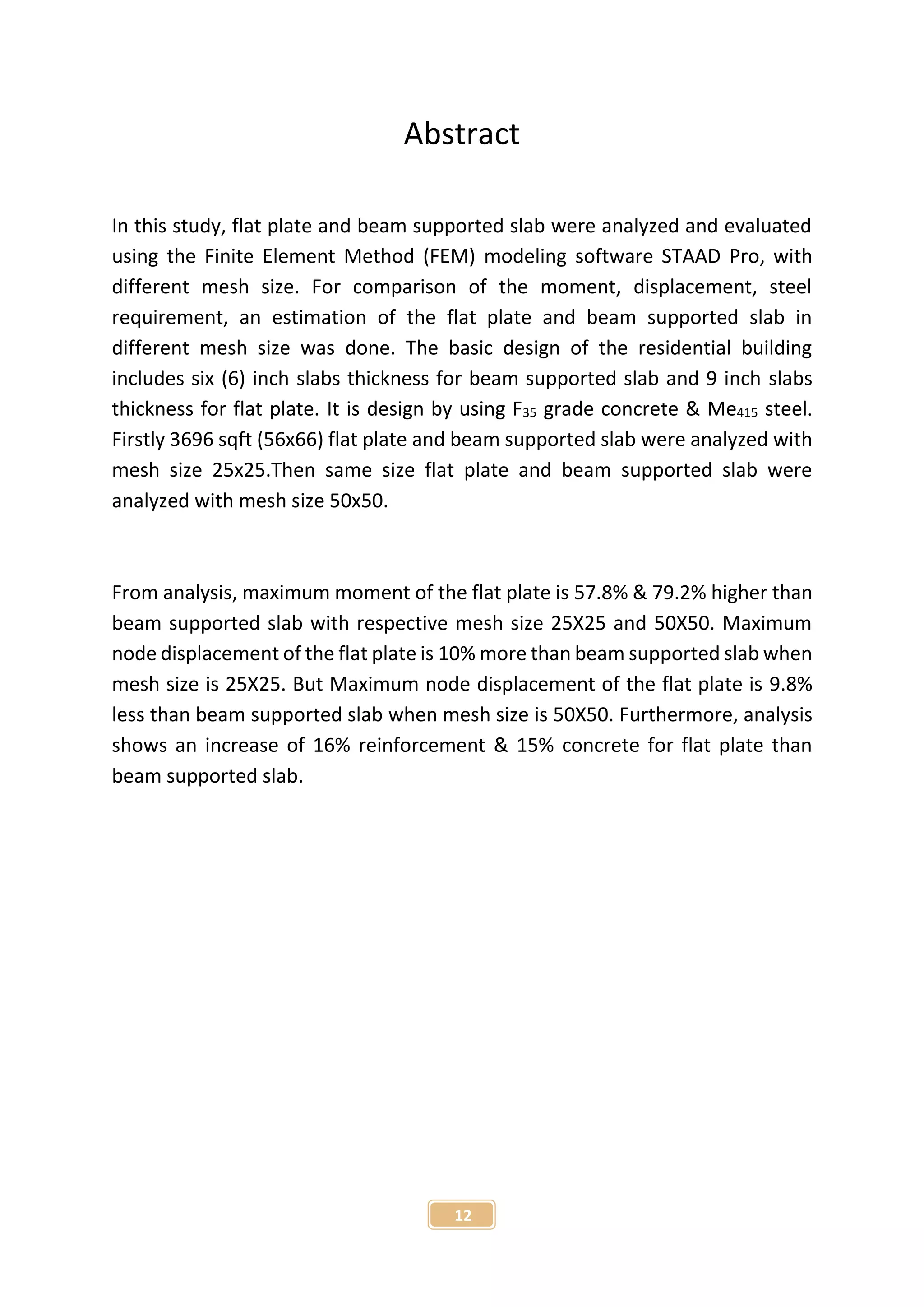
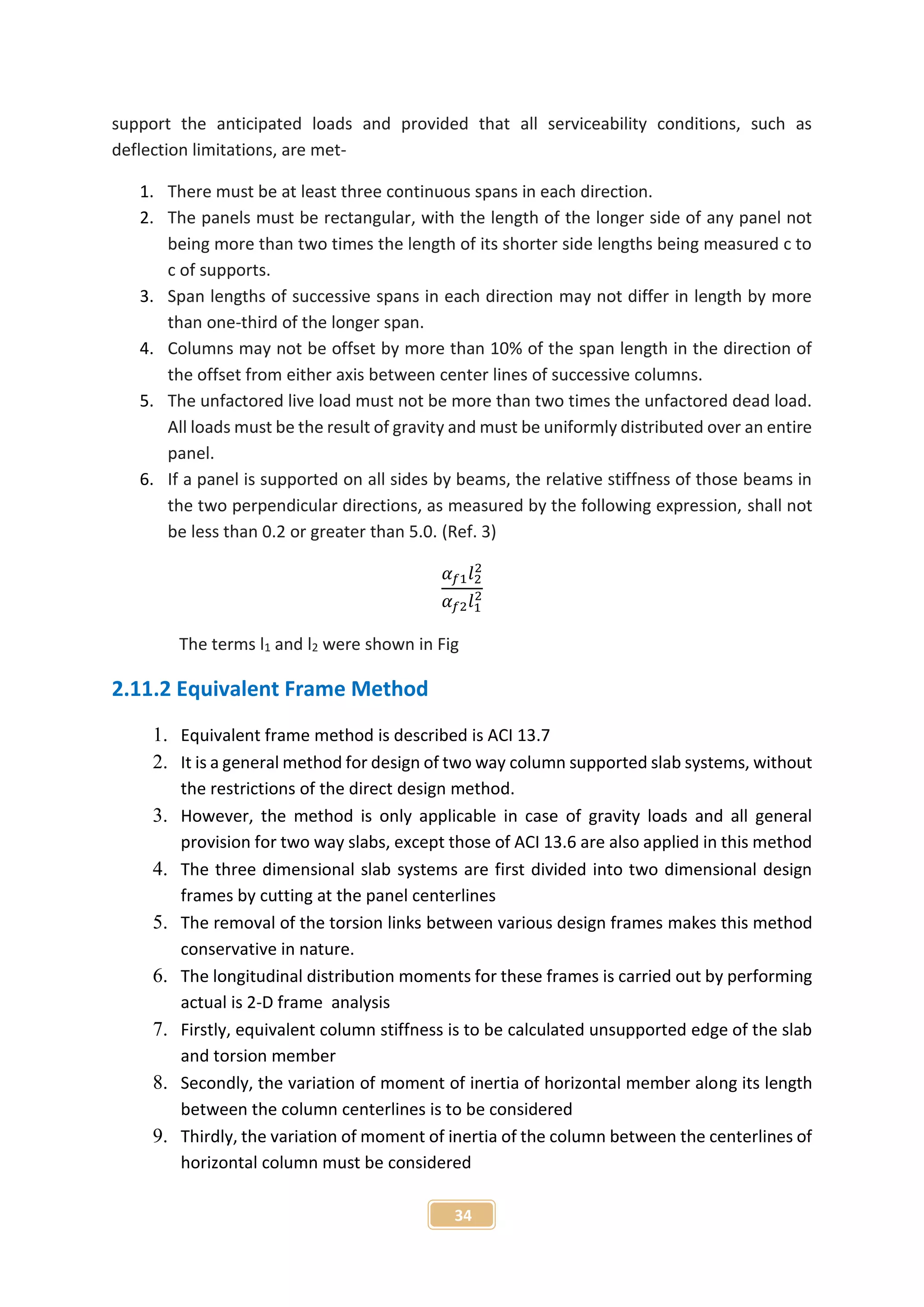
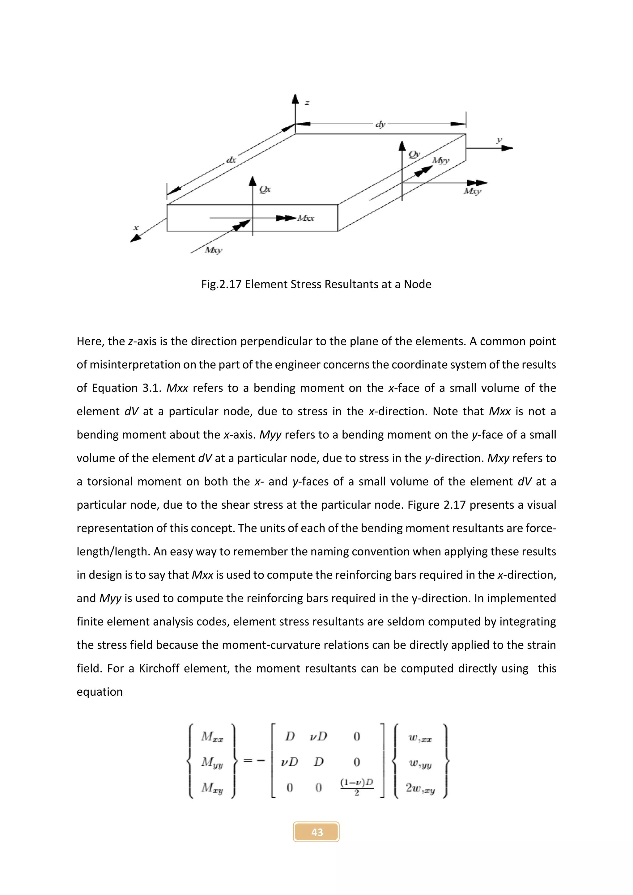
Fig. 2.19 Average Bending Moment Resultants at Each Node along Cut
In this equation, the average moment resultants from each node, Mrx,i, are averaged and
then multiplied by the width of the cut to compute the entire resultant moment acting on the
cross-section [29]. Once the resultant design moment has been computed, flexural
reinforcement is designed according to ACI 318 as explained in Section 2.1. The resultant
bending moment for the design of reinforcement in the y-direction is similarly computed
using Equation 3.9 by replacing Mrx,i with Mry,i.
2.11.4.5 Design
1. After analysis a structure has to be designed to carry loads acting on it considering a
certain factor of safety .
2. In India United Kingdom, USA, French, German, European structures are designed by
using their codes for both concrete and steel structures.

49
3. The design in STAAD.Pro supports over 70 international codes and over 20 U.S. codes
in 7 languages.
4. After designing the structure it is again analyzed and results of analysis for each beam
and column is shown in the output file
2.11.4.6 Conclusion
 Staad pro is widely used by most of the organization for their construction needs.
 Unfortunately, well skilled staad pro engineers are very hard to search.
 If we believe in the prediction of the industry experts then those students who
will be getting trained on staad pro in the current and upcoming two years will
have bright and successful career ahead in the real estate and construction
domain
 By attending this training in STAAD.Pro we were able to learn various features of
STAAD.Pro which will be very helpful in the near future

50
Chapter 3
Design Methodology
3.1 General
STAAD or (STAAD.Pro) is a structural analysis and design computer program originally
developed by Research Engineers International at Yorba Linda, CA in year 1997. In late 2005,
Research Engineers International was bought by Bentley Systems.
An older version called Staad-III for windows is used by Iowa State University for educational
purposes for civil and structural engineers. Initially it was used for DOS-Window system.
Design any type of structure and share your synchronized model data with confidence
among entire design team, using STAAD Pro. Ensure on time and on budget completion of
steel, concrete, timber, aluminum, and cold-formed steel projects, regardless of complexity.
This software can confidently design structures anywhere in the world using over 80
international codes, reducing to learn multiple software applications. Thanks to the flexible
modeling environment and advanced features such as dynamic change revisions and
management
o Lower total cost of ownership: Design any type of structure including culverts,
petrochemical plants, tunnels, bridges, and piles
o Increase design productivity: Streamline your workflows to reduce duplication of
effort and eliminate errors
o Reduce project costs and delays: Provide accurate and economical designs to your
clients and quickly turnaround change requests

51
3.2 Plan of Flat Plate & Beam Supported Slab
Fig. 3.1 plan of the flat plat & beam supported slab

52
3.3 Flat Plate Design
The structure for this project is a slab fixed along two edges. We will model it using 25
quadrilateral (4-noded) plate elements. The structure and the mathematical model are shown
in the figures below. It is subjected to self weight, pressure loads and temperature loads. Our
goal is to create the model, assign all required input, perform the analysis, and go through
the results.
3.4 Basic Data for the Structure
3.5 Design Procedure by Staad Pro.
Starting the program 1. Select the STAAD Pro. icon from the STAAD Pro. V8i program group
found in the Windows Start menu. The STAAD Pro. window opens to the start screen. Figure2-
259:TheSTAAD.Prowindowdisplayingthestartscreen
Fig.3.2 starting page of Staad Pro.
Attribute Data
Element
properties
Slab is 9” thick
Material
Constants
E, Density, Poisson, Alpha – Default values for concrete
Primary Loads LL=40 Psi , PW= 50Psi, FF=25Psi,
Combination
Loads
1.4DL+ 1.7LL
Analysis Type Linear Elastic

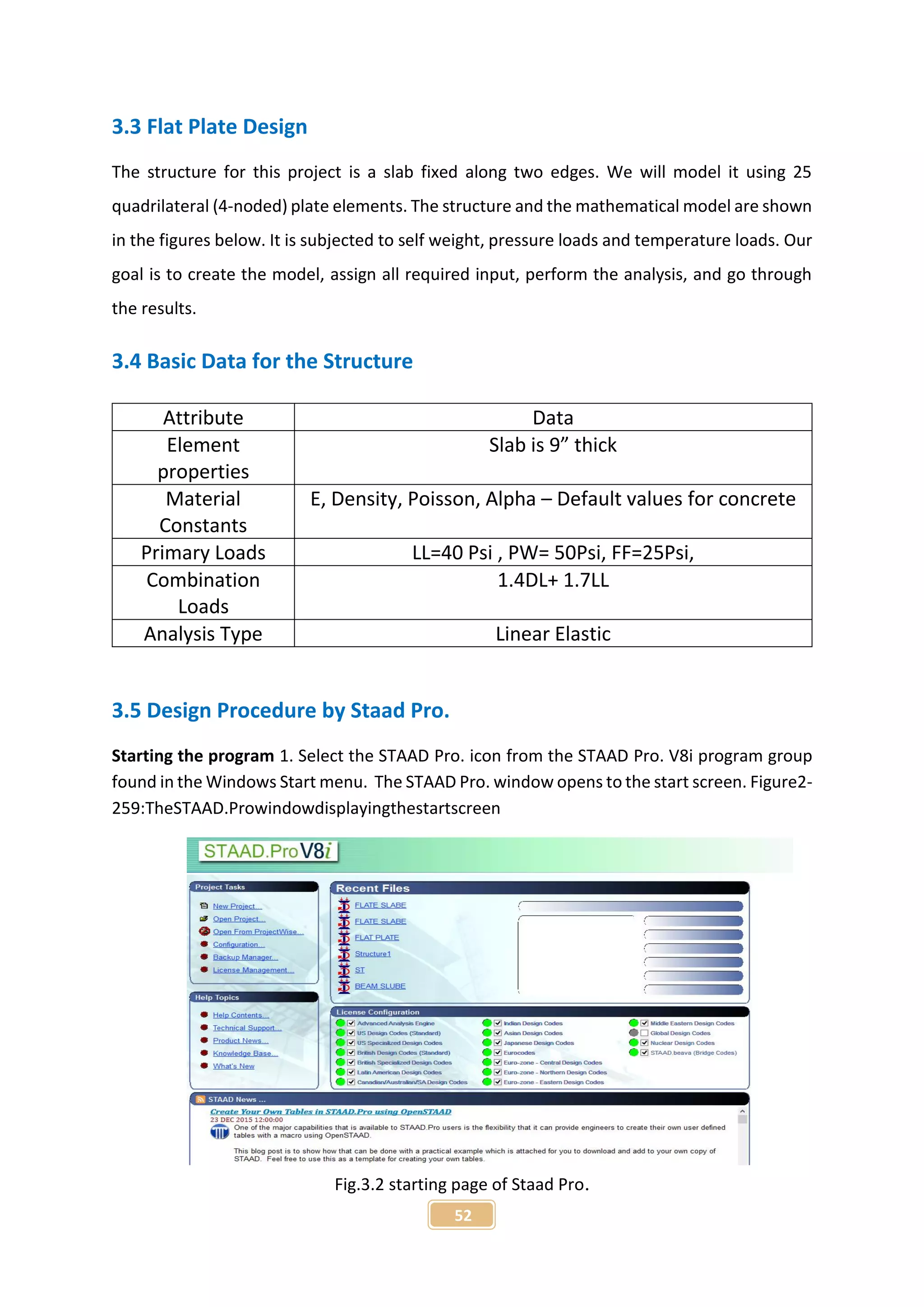
53
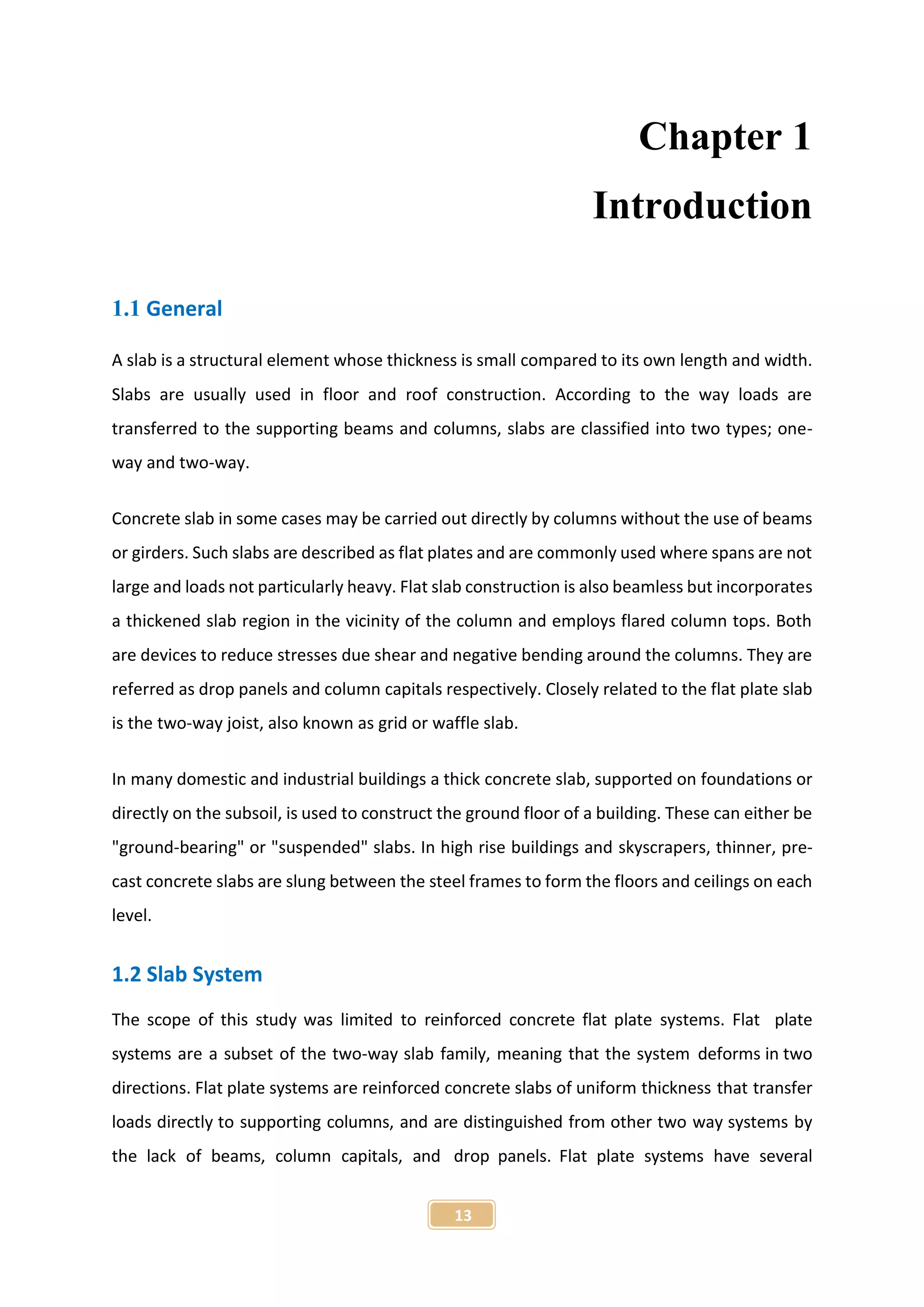
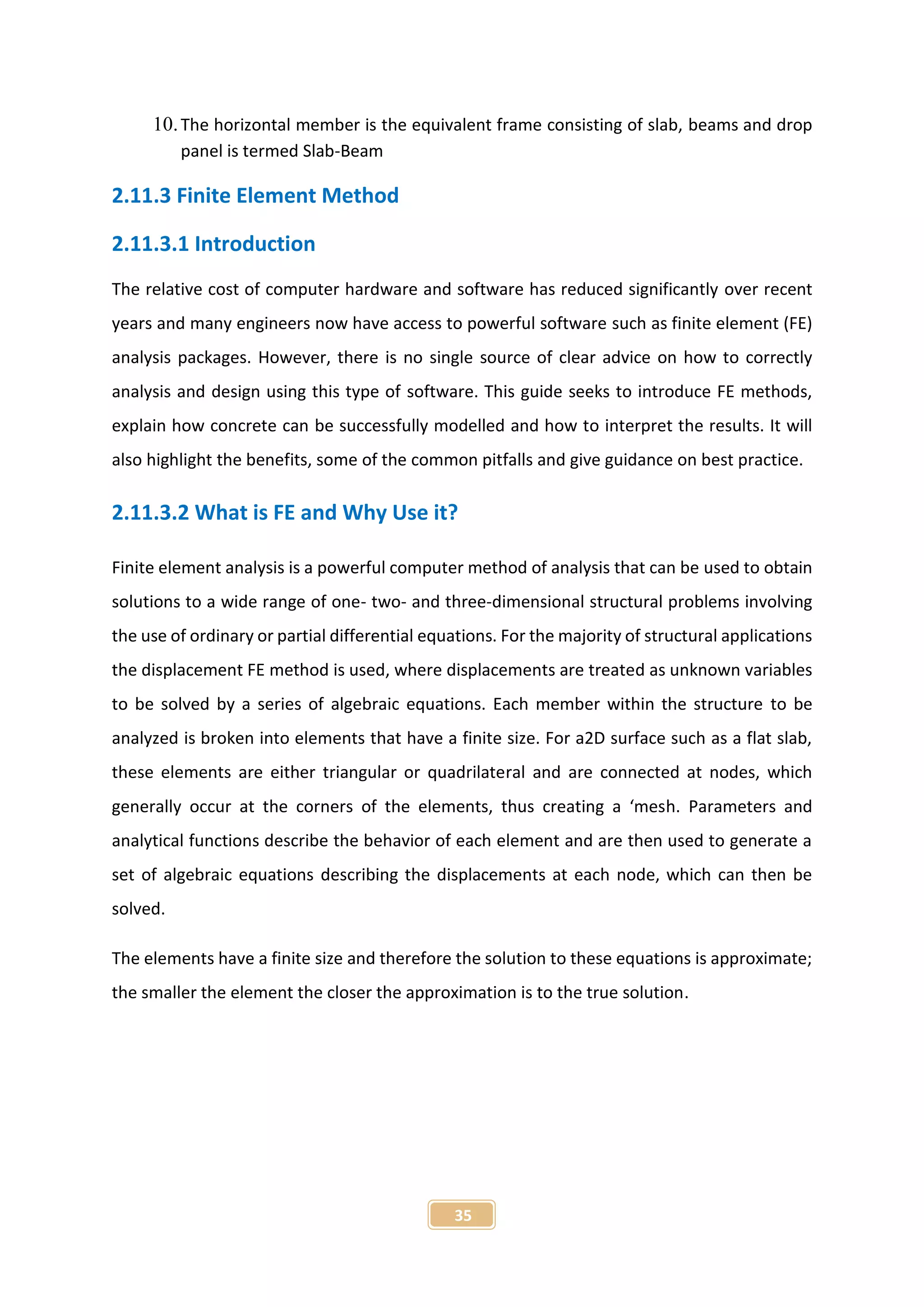
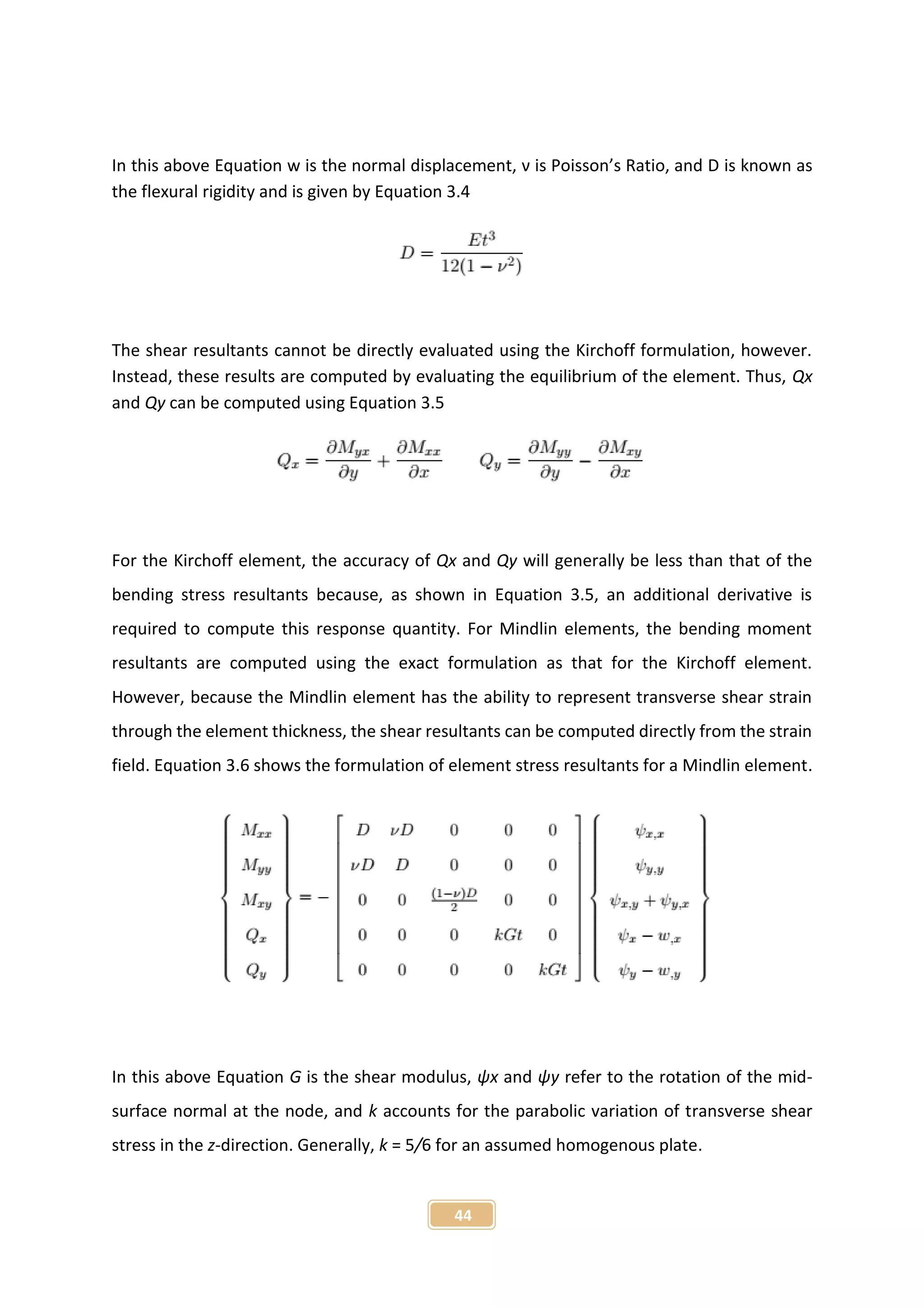
Creating a new structure In the New dialog, we provide some crucial initial data necessary
for building the model. 1. Select File > New or select New Project under Project Tasks.
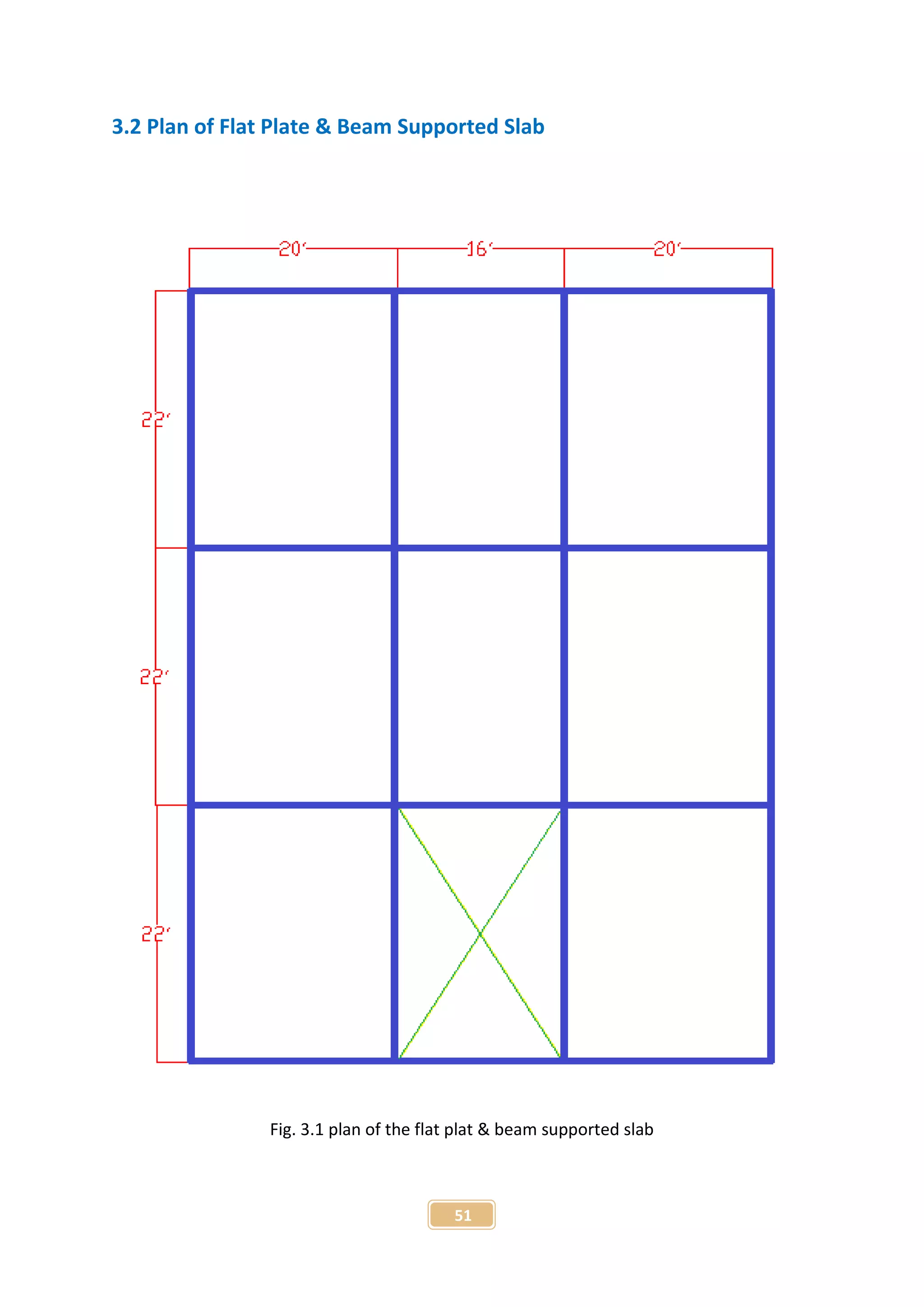
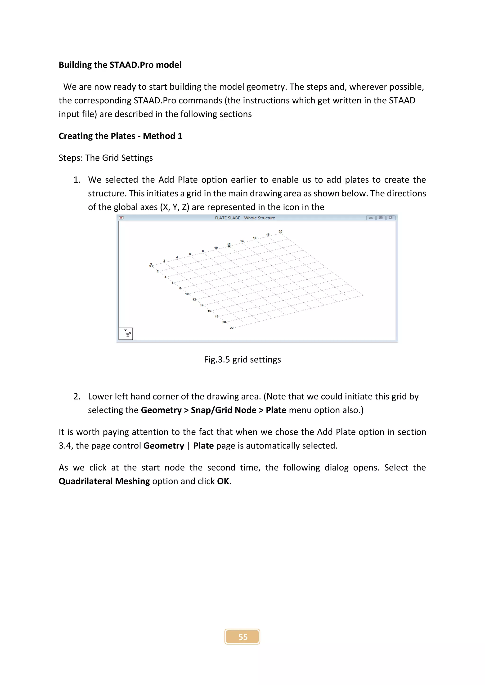
Fig.3.3 Selected Plane
The structure type is defined as either Space, Plane, Floor, or Truss:
Space the structure, the loading or both, cause the structure to deform in all 3 global axes (X,
Y and Z).
Plane the geometry, loading and deformation are restricted to the global X-Y plane only
Floor a structure whose geometry is confined to the X-Z plane. Truss the structure carries
loading by pure axial action. Truss members are deemed incapable of carrying shear, bending
and torsion.
2. Select Space.
3. Select Meter as the length unit and Kilo Newton as the force unit.
Hints: The units can be changed later if necessary, at any stage of the model
creation.
4. Specify the File Name as Plates Tutorial and specify a Location where the STAAD input
file will be located on your computer or network.
You can directly type a file path or click […] to open the Browse by Folder dialog, which
is used to select a location using a Windows file tree. After specifying the above input,
click Next.
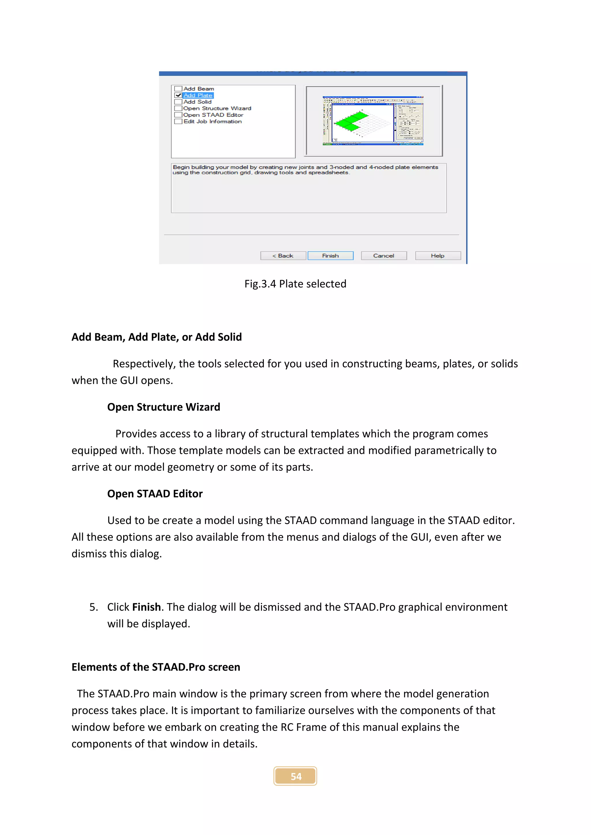
The next page of the wizard, Where do you want to go? opens
5. Set the Add Plate check box

54
Fig.3.4 Plate selected
Add Beam, Add Plate, or Add Solid
Respectively, the tools selected for you used in constructing beams, plates, or solids
when the GUI opens.
Open Structure Wizard
Provides access to a library of structural templates which the program comes
equipped with. Those template models can be extracted and modified parametrically to
arrive at our model geometry or some of its parts.
Open STAAD Editor
Used to be create a model using the STAAD command language in the STAAD editor.
All these options are also available from the menus and dialogs of the GUI, even after we
dismiss this dialog.
5. Click Finish. The dialog will be dismissed and the STAAD.Pro graphical environment
will be displayed.
Elements of the STAAD.Pro screen
The STAAD.Pro main window is the primary screen from where the model generation
process takes place. It is important to familiarize ourselves with the components of that
window before we embark on creating the RC Frame of this manual explains the
components of that window in details.

55
Building the STAAD.Pro model
We are now ready to start building the model geometry. The steps and, wherever possible,
the corresponding STAAD.Pro commands (the instructions which get written in the STAAD
input file) are described in the following sections
Creating the Plates - Method 1
Steps: The Grid Settings
1. We selected the Add Plate option earlier to enable us to add plates to create the
structure. This initiates a grid in the main drawing area as shown below. The directions
of the global axes (X, Y, Z) are represented in the icon in the
Fig.3.5 grid settings
2. Lower left hand corner of the drawing area. (Note that we could initiate this grid by
selecting the Geometry > Snap/Grid Node > Plate menu option also.)
It is worth paying attention to the fact that when we chose the Add Plate option in section
3.4, the page control Geometry | Plate page is automatically selected.
As we click at the start node the second time, the following dialog opens. Select the
Quadrilateral Meshing option and click OK.

56
Fig. 3.6 Mesh setting page
The Select Meshing Parameters dialog (as we saw earlier in Method 3), comes up. Notice that
this time however, the data for the four corners is automatically filled in. The program used
the coordinates of the four nodes we selected to define A, B, C, and D. Provide the Bias and
the Divisions of the model as shown in the figure below. Click Apply.
As we click Apply, our model will appear in the drawing area as the one shown below.
Press the ESC key to exit the mesh generating mode.
Fig.3.7 Thickness settings
At this point, the Properties dialog will look as shown below.
The structure will now look as shown below.

57
Fig.3.8Assign to plate
Click anywhere in the drawing area to un-highlight the selected entities. We do this only as a
safety precaution. When an entity is highlighted, clicking on any Assign option is liable to
cause an undesired attribute to be assigned to that entity.
Fig.3.9 same plate thickness
1. In either case, the Supports dialog opens as shown in the next figure.
2. For easy identification of the nodes where we wish to place the supports,
toggle the display of the Node Numbers on.
3. Since we already know that nodes 1, 2, 5, 7, 4 and 10 are to be associated

58
with the Fixed support, using the Nodes Cursor , select these nodes.
4. Then, click Create in the Supports dialog as shown below.
Fig. 3.10 support reaction
Note: It is important to understand that the Assign button is active because of what we did
in step 4 earlier. Had we not selected the nodes before reaching this point, this option
would not have been active.
After the supports have been assigned, the structure will look like the one shown below.
Fig.3.11 Assigned Support
Load Cases Notice that the pressure load value listed in the beginning of this tutorial is in KN
and meter units. Rather than convert that value to the current input units, we will conform
to those units. The current input units, which we last set while specifying THICKNESS was
CENTIMETER. We have to change the force unit to Kilogram and the length units to Meter. To
change the units, as before, select the Input Units tool from the top toolbar, or select the
Tools > Set Current input Unit menu option from the top menu bar. In the Set Current input

59
Units dialog that comes up, specify the length units as Meter and the force units as Kilogram.
Window titled “Load” appears on the right-hand side of the screen. To initiate the first load
case, highlight Load Case Details and click Add.
Fig. 3.12 Load case
Load Definition the newly created load case will now appear under the Load Cases Details in
the Load dialog.
Fig. 3.13 Load definition
In the Add New Load Items dialog, select the Self weight Load option under the Self weight
item. Specify the Direction as Y, and the Factor as -1.0 the negative number signifies that the
self-weight load acts opposite to the positive direction of the global axis (Y in this case) along
which it is applied. Click Add. The self-weight load is applicable to every member of the
structure, and cannot be applied on a selected list of members.

60
Fig. 3.14 Self Weight
Next, let us initiate the creation of the second load case which is a pressure load on the
elements. To do this, highlight Load Case Details in the Add New Load Cases dialog, once
again, we are not associating the load case we are about to create with any code based
Loading Type and so, leave that box as none. Specify the Title of the second load case as
External Pressure Load and click Add.
Fig. 3.15 Pressure on plate
Since the pressure load is to be applied on all the elements of the model, the easiest way to
do that is to set the Assignment Method to Assign to View. Then, click Assign in the Load
dialog as shown below.

61
Fig.3.16 Flat slab whole structure
Click Define Commands in the data area on the right hand side of the screen. The
Analysis/Print Commands dialog opens.
Fig. 3.17 load of partition wall
Next, let us create the third load case which is a temperature load. The initiation of a new
load case is best done using the procedure explained in step 7. In the dialog that comes up,
let us specify the Title of the third load case as Temperature Load and click Add.

62
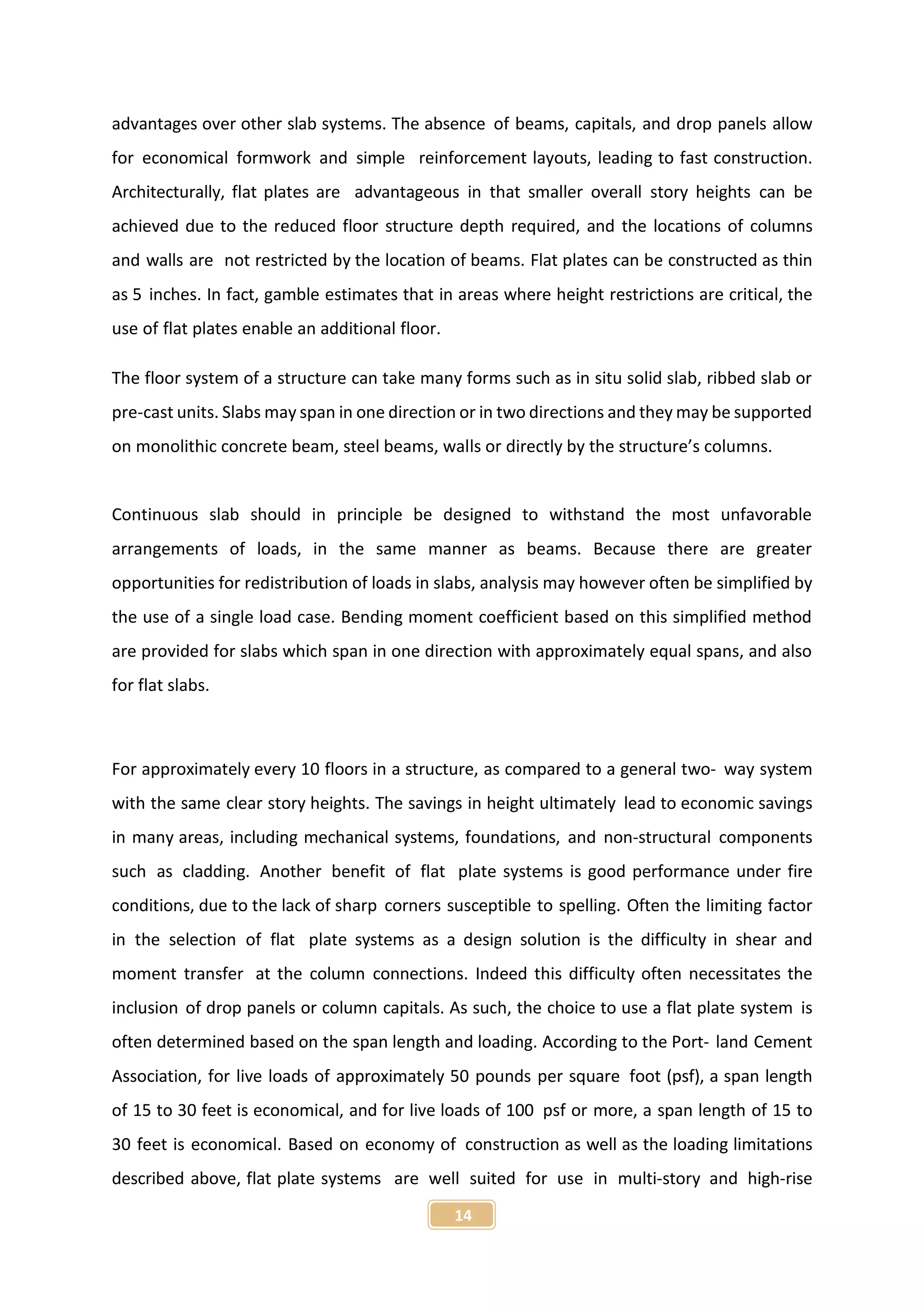
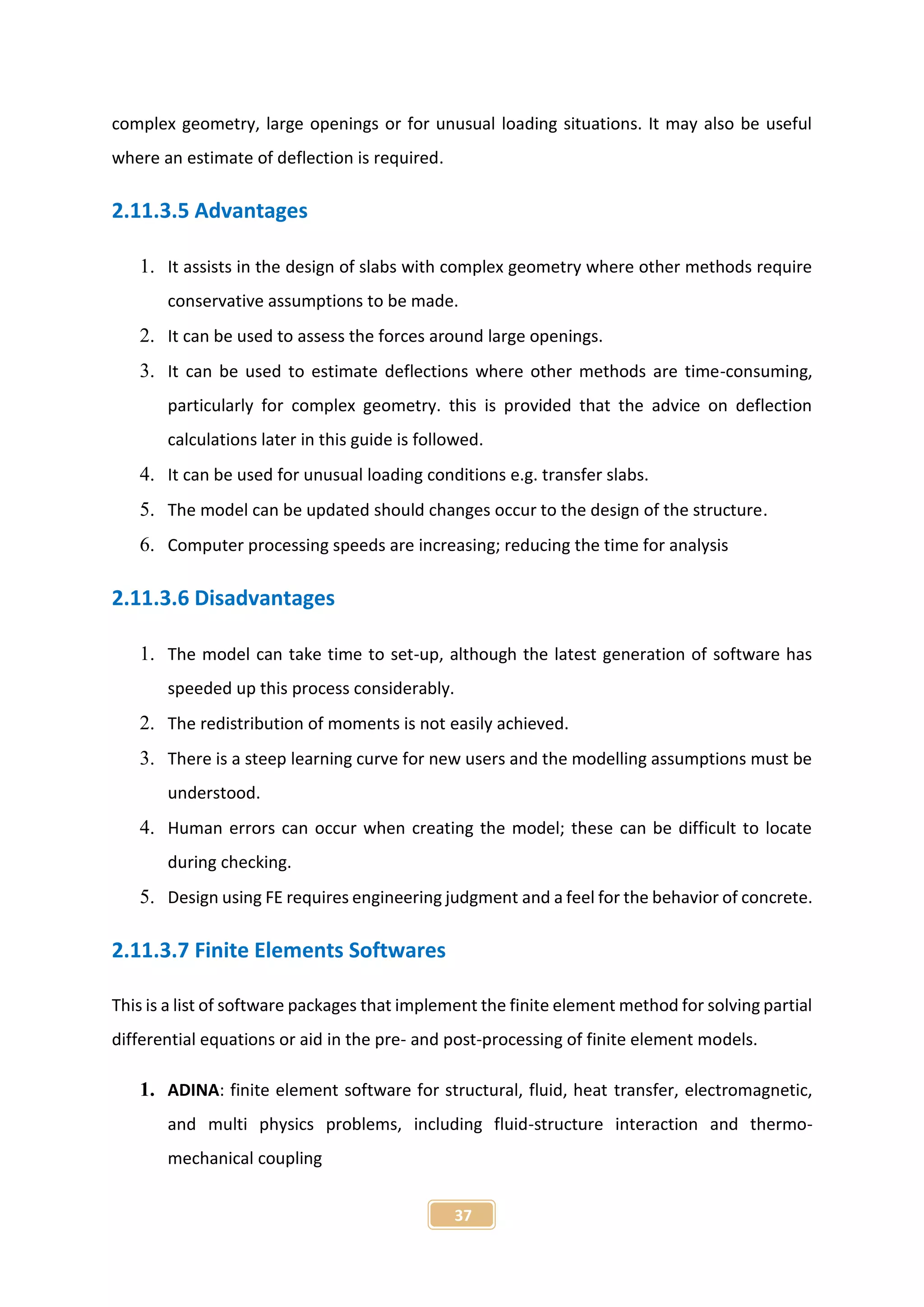
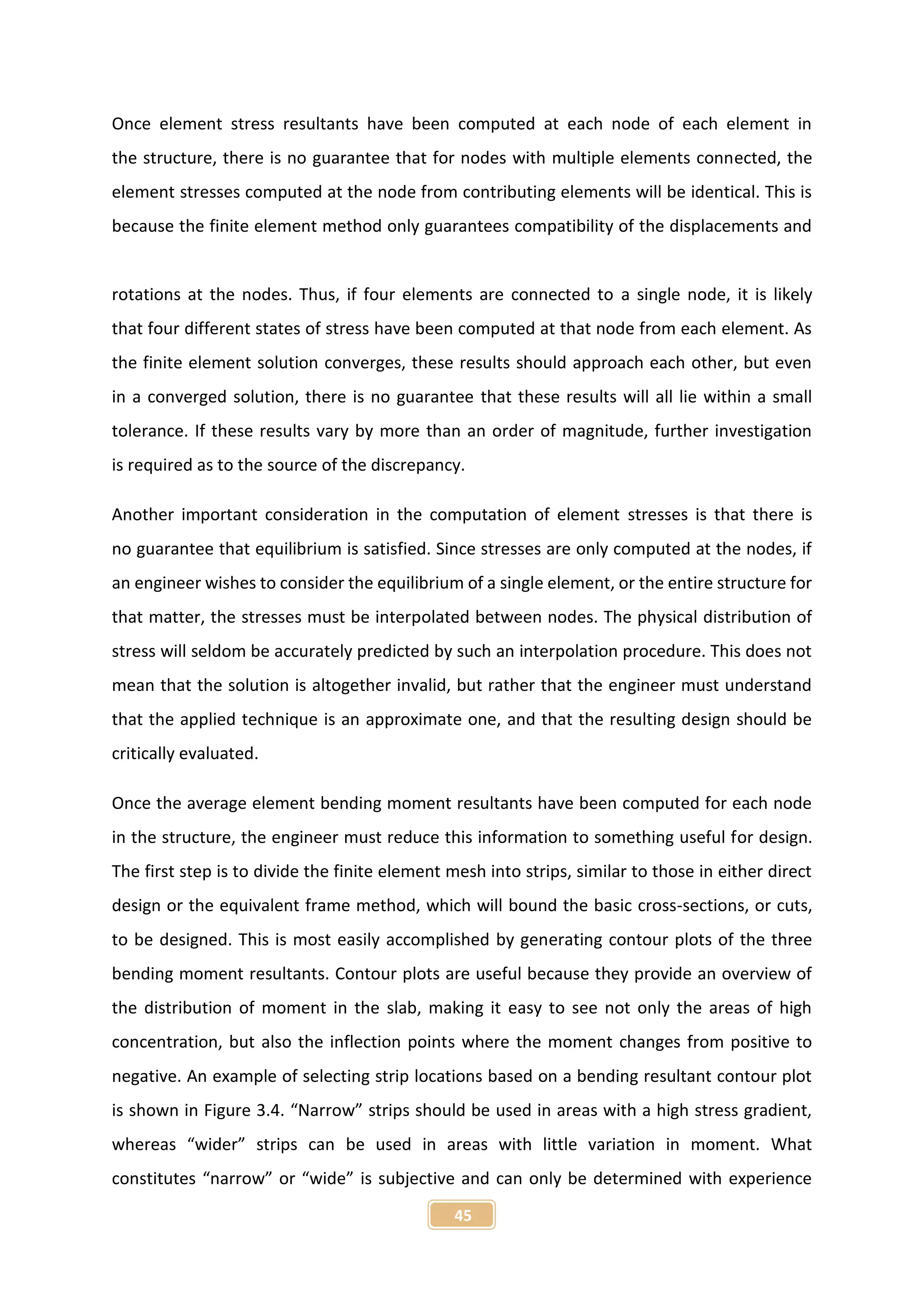
Fig. 3.18 Load combination
Next, in the Define Combinations box, select load case 1 from the left side list box and click
[>]. Repeat this with load case 2 also. Load cases 1 and 2 will appear in the right side list
box as shown in the figure below. (These data indicate that we are adding the two load cases
with a multiplication factor of 1.0 and that the load combination results would be obtained
by algebraic summation of the results for individual load cases.) Finally, click Add.
Fig. 3.19 Load combination
To initiate and define load case 5 as a load combination, as before, enter the Load No: as 102
and the Title as Case 1 + Case 3.
Next, repeat step 2 except for selecting load cases 1 and 3 instead of cases 1 and 2.

63
Fig. 3.20 Analysis
Thus, load 102 is also created. If we change our mind about the composition of any existing
combination case, we can select the case we want to alter, and make the necessary changes
in terms of the constituent cases or their factors.
Fig. 3.21 Analysis Structure

64
Hint:Remember to save your work by either selecting File > Save, the Save tool, or pressing
CTRL+S.
Fig. 3.22 Analysis/print
Click Define Commands in the data area on the right hand side of the screen. The
Analysis/Print Commands dialog opens.
3.6 Analysis of a plate
Fig. 3.23 View output file

65
At the end of these calculations, two activities take place. a) A Done button becomes active
b) three options become available at the bottom left corner of this information window.
The View Output File option allows us to view the output file created by STAAD. The output
file contains the numerical results produced in response to the various input commands we
specified during the model generation process. It also tells us whether any errors were
encountered, and if so, whether the analysis and design was successfully completed or not.
Section 3.10 (also, see section 1.9) offers additional details on viewing and understanding the
contents of the output file. The Go to Post Processing Mode option allows us to go to graphical
part of the program known as the Post-processor. This is where one can extensively verify the
results, view the results graphically, plot result diagrams, produce reports, etc. Section 3.11
explains the Post processing mode in greater detail. The Stay in Modelling Mode lets us
continue to be in the Model generation mode of the program (the one we currently are in) in
case we wish to make further changes to our model.
3.7 Viewing the output file
During the analysis stage, an output file containing results, warnings and messages associated
with errors if any in the output, is produced. This file has the extension .anl and may be viewed
using the output viewer. See Appendix A
3.8 Post-Processing
If there are no errors in the input, the analysis is successfully completed. The extensive
facilities of the Post-processing mode can then be used to view the results graphically and
numerically assess the suitability of the structure from the standpoint of safety, serviceability
and efficiency create customized reports and plots the procedure for entering the post
processing mode is explained in section of this manual. Node results such as displacements
and support reactions are available for all models. The methods explained in the first two
tutorials – see sections– may be used to explore these. If beams are present in the model,
beam results will be available too For this example, we will look at the support reactions. We
do not have any beams in our model, so no results will be available for this type of entity. For
plates, the results available are stresses, and “unit width” moments. There are several
different methods for viewing these results, as explained in the next few sections.

66
Viewing stress values in a tabular form
1. Select View > Tables or Right-click in the View window and select Tables from the pop-up
menu. The Tables dialog opens.
Fig.3.24 Viewing stress values in a tabular form
2. Select Plate Center Stress and click OK. The Plate Center Stress table opens.
Fig. 3.25 The Plate Center Stress table
The table has the following tabs:
Shear, Membrane and Bending
These terms are explained in Section 1.6.1 of the STAAD Technical Reference Manual. The
individual values for each plate for each selected load case are displayed.

67
This tab contains the maximum for each of the 8 values listed in the Shear, Membrane and
Bending tab.
Principal and Von Mises
These terms too are explained in Section 1.6.1 of the STAAD Technical Reference Manual. The
individual values for each plate for each selected load case are displayed, for the top and
bottom surfaces of the elements.
Summary
This tab contains the maximum for each of the 8 values listed in the Principal and Von Mises
tab. Global Moments This tab provides the moments about the global X, Y and Z axes at the
center of each element.
Stress Contours
Stress contours are a color-based plot of the variation of stress or moment across the surface
of the slab or a selected portion of it. There are 2 ways to switch on stress contour plots:
1. Select either
The Plate | Contour page
Select Results > Plate Stress Contour.
The Diagrams dialog opens
2. From the Stress type field, select the specific type of stress for which you want the
contour drawn.
3. From the Load Case selection box, select the load case number.
Stress values are known exactly only at the plate centroid locations. Everywhere else,
they are calculated by linear interpolation between the center point stress values of
adjacent plates. The Enhanced type contour chooses a larger number of points
compared to the Normal type contour in determining the stress variation.
4. View Stress Index will display a small table consisting of the numerical range of values
from smallest to largest which are represented in the plot. Let us set the following:

68
Fig.3.26 stress contour
 Load case – 102
 Stress Type – Von Mis Top
 Contour Type – Normal Fill
 Index based on Center Stress
 View Stress Index
 Re-Index for new view
Fig.3.27 stress contour

69
Fig.3.28 Flat slab
The following diagram will be displayed. We can keep changing the settings and click on
apply to see all the various possible results in the above facility.
Viewing plate results using element query
Element Query is a facility where several results for a specific element can be viewed at the
same time from a single dialog. Let us explore this facility for element 4.
1. Select the Plate Cursor tool.
2. Double-click on element
or
Select element 4 and then select Tools > Query > Plate.
The Plate dialog opens.
The various tabs of the query box enable one to view various types of information such as the
plate geometry, property constants, stresses, etc., for various load cases, as well as print those
values.
Some example tabs of this dialog.

70
Fig. 3.29 plate edge length & area
Fig. 3.30 plate stress
Producing an onscreen report
Occasionally, we will come across a need to obtain results conforming to certain restrictions,
such as, say, the resultant node displacements for a few selected nodes, for a few selected
load cases, sorted in the order from low to high, with the values reported in a tabular form.
The facility which enables us to obtain such customized on-screen results is the Report
menu on top of the screen.
Let us produce a report consisting of the plate principal stresses, for all plates, sorted in the
order from Low to High of the Principal Maximum Stress (SMAX) for load combined.

71
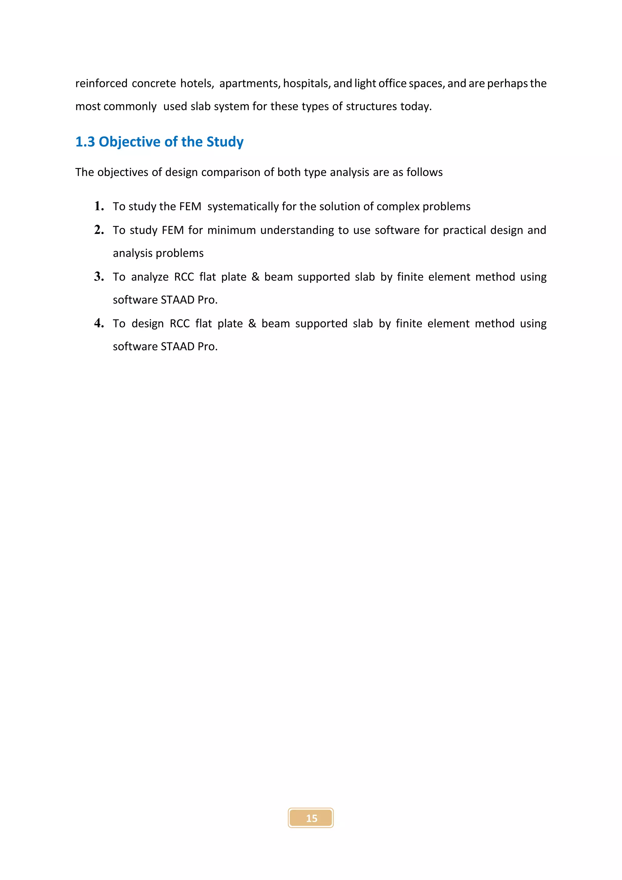
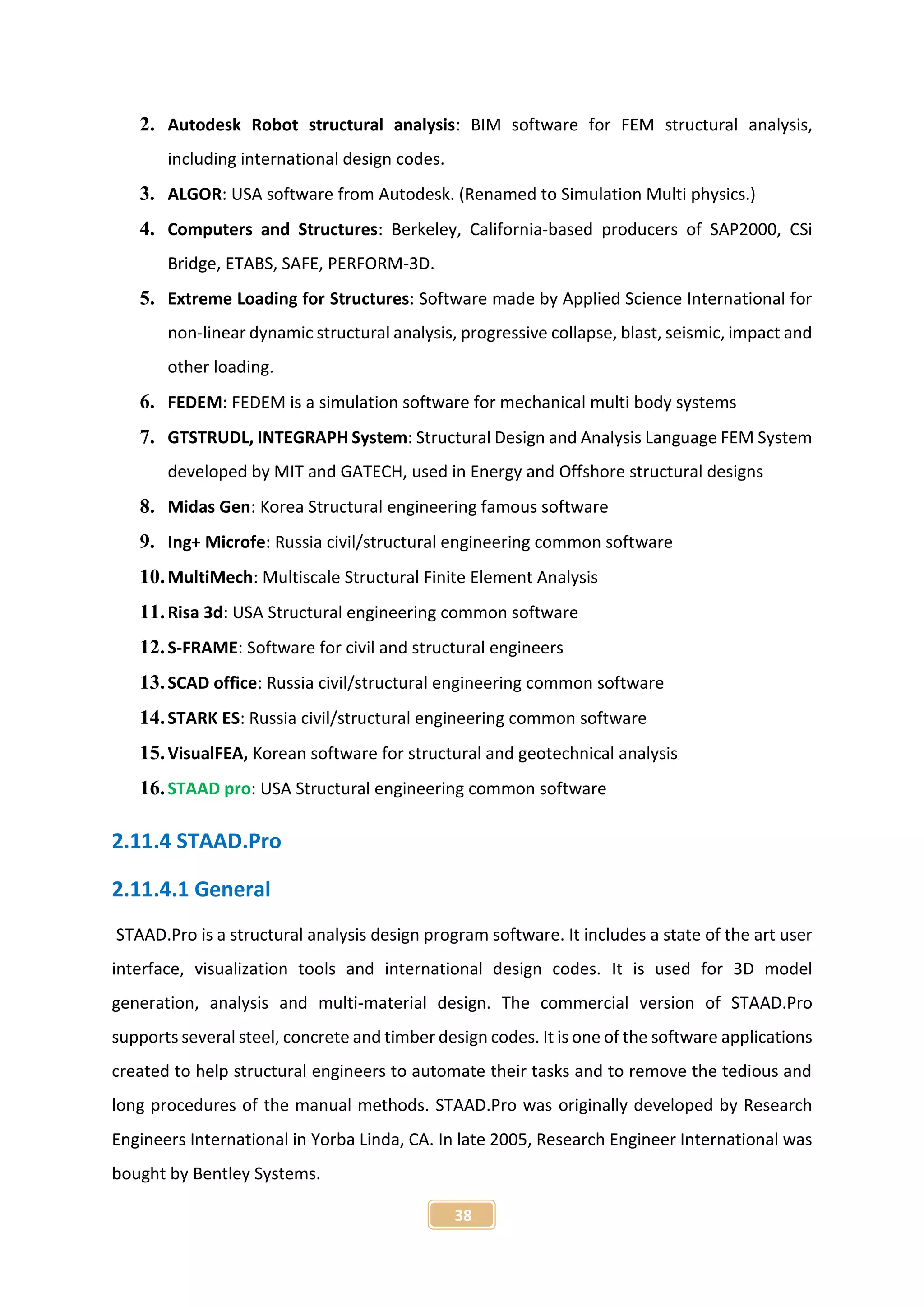
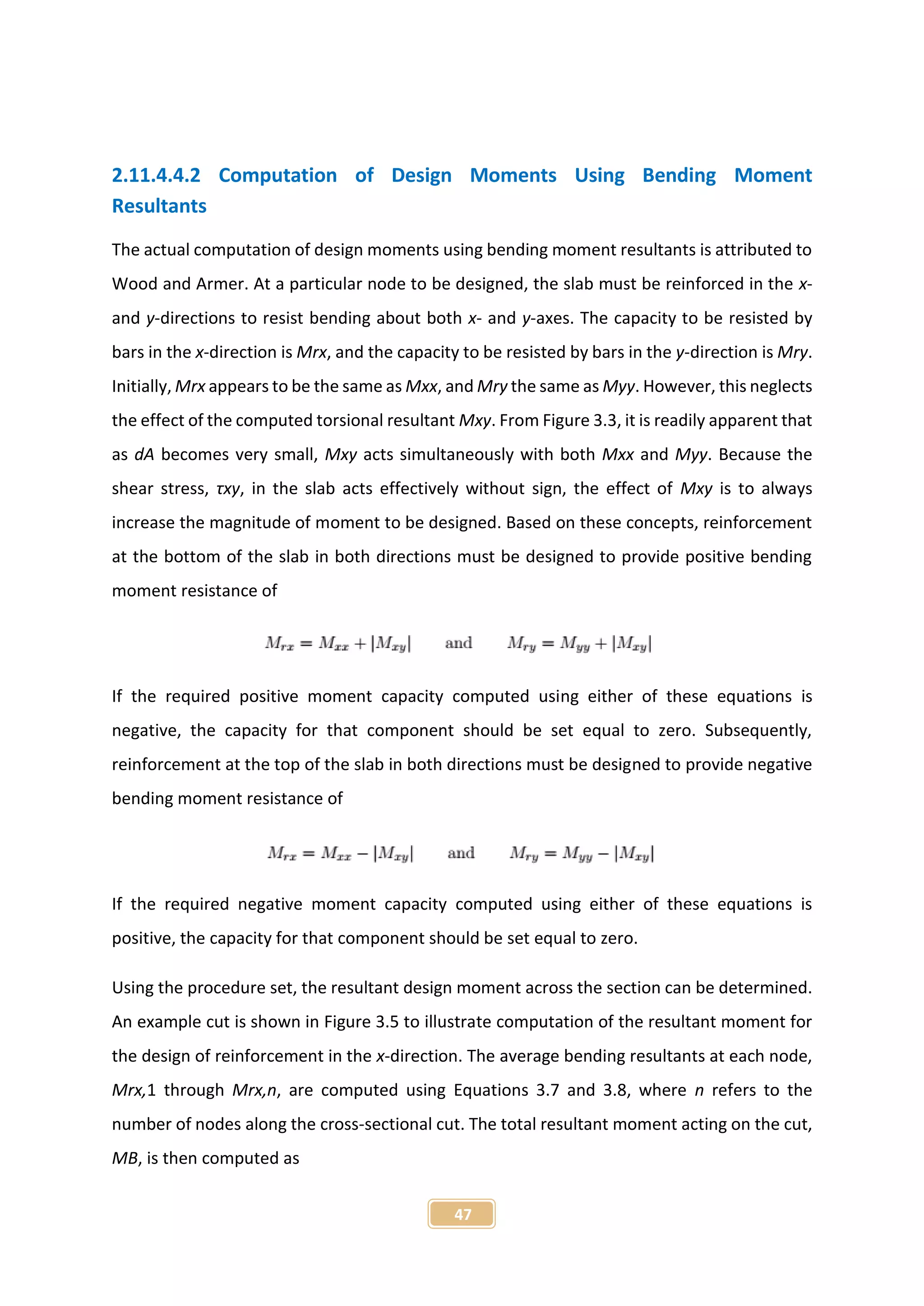
1. Select all the plates using the Plates Cursor.
2. Select Report > Plate Results > Principal Stresses.
Fig.3.31 Plate force
3. Select the Loading tab.
4. Select load cases COMBINED in the Available list and click [>] to add them to the Selected
list.
5. Select the Sorting tab. Choose SMAX under the Sort by Plate Stress category and select
List from Low to High as the Set Sorting Order
Fig. 3.32 Plate force
6. (Optional) If you wish to save this report for future use, select the Report tab, provide a
title for the report, and set the Save ID check box.
7. Click OK.

72
The following figure shows the table of maximum principal stress with SMAX values sorted
from Low to High.
Fig. 3.33 Plate force
8. To print this table, right-click anywhere within the table and select Print from the pop-up
menu.
Select the print option to get a hardcopy of the report.
To transfer the contents of this table to a Microsoft Excel file
1. Click at the top left corner of the table with the left mouse button. The entire table will
become highlighted.
2. Right click and select Copy from the pop-up menu.
3. Open an Excel worksheet, click at the desired cell and Paste the contents.
Viewing Support Reactions
Since supports are located at nodes of the structure, results of this type are available along
with other node results such as displacements.
1. Select the Node | Reactions page on the left side of the screen.
The six values — namely, the three forces along global X, Y and Z, and the three moments Mx,
My and Mz, in the global axis system — are displayed in a box for each support node.
Display of one or more of the six terms of each support node may be toggled off in the
following manner.
1. Select Results > View Value…. The Annotation dialog opens.
2. Select the Reactions tab. clear the Global X and Global Z check boxes in the direct
category.

73
3. Click Annotate and then Close. The drawing will now contain only the remaining 4
terms (see figure below).
Fig. 3.34 moment value diagram
The table on the right side of the screen contains the reaction values for all supports for all
selected load cases
Fig. 3.35 Force & Moment table
This table can also be displayed from any mode by clicking on the View menu, choosing Tables,
and switching on Support Reactions.

74
The method explained in section 3.11.3 may be used to change the units in which these values
are displayed. The summary tab contains the maximum value for each of the 6 degrees of
freedom along with the load case number responsible for it.
Fig. 3.36 Force & Moment table
This brings us to the conclusion of this tutorial. Additional help on using plates is available in
Examples 9, 10 and 18 in the Examples Manual
3.9 Staad Pro. Output File for Beam supported slab
See Appendix B

75
Chapter 4
Results & Discussions
4.1 General
The forces and displacements developed of the flat plate and beam supported slab of the
structure are got from the analysis with different mesh size. These results obtained from the
analysis have been discussed details in this chapter. Further these results have been used for
the understanding of the behavior of the structure between the beam supported slab and flat
plate under the effects of vertical loads.
In this part of the document analysis and results for Mesh analysis results, moment analysis,
displacement analysis, and stress analysis are discussed.
Results
 From moment analysis results it can be observed that the flat plate is higher than
beam supported slab with respectively mesh size 25X25 and 50X50. At 25x25 mesh
size, the maximum moment of the flat plate is 57.8% more than that of the beam
supported slab and 50X50 mesh size, the maximum moment of the flat plate is 79.2%
more than that of the beam supported slab.
 From node displacement analysis results it can be observed that of the flat plate is
more than beam supported slab when mesh size 25X25. But Maximum node
displacement of the flat plate is less than beam supported when mesh size 50X50.
Finally it can be observed that, the node displacement of the flat plate will decrease
as the mesh size increases.
 Flat plate slab is thicker and more heavily reinforced than slabs with beams and
girders. Almost16% more reinforcement are used for flat plate structure than beam
supported structure.
 Almost 15% more concrete are used for flat plate structure than beam supported
structure

76
4.2 Mesh Analysis
4.2.1 Summary of Flat Plat & Beam Supported Slab (25x25 Mesh)
Summary of table for flat plate center stress mesh analysis (25x25)
Qx Qy Sx Sy Sxy Mx My Mxy
(psi) (psi) (psi) (psi) (psi) (lb
-
in/in) (lb
-
in/in) (lb
-
in/in)
Max Qx 1106 5:1.4DL+1.7LL 386.067 -333.62 0 0 0 -26.3E 3 -32.1E 3 2.26E 3
Min Qx 1694 5:1.4DL+1.7LL -276.73 -168.68 0 0 0 -22.9E 3 -18.5E 3 -12.3E 3
Max Qy 3336 5:1.4DL+1.7LL 386.067 333.617 0 0 0 -26.3E 3 -32.1E 3 -2.26E 3
Min Qy 1106 5:1.4DL+1.7LL 386.067 -333.62 0 0 0 -26.3E 3 -32.1E 3 2.26E 3
Max Sx 35 1:SW 0 0 0 0 0 0 0 0
Min Sx 35 1:SW 0 0 0 0 0 0 0 0
Max Sy 35 1:SW 0 0 0 0 0 0 0 0
Min Sy 35 1:SW 0 0 0 0 0 0 0 0
Max Sxy 35 1:SW 0 0 0 0 0 0 0 0
Min Sxy 35 1:SW 0 0 0 0 0 0 0 0
Max Mx 53 5:1.4DL+1.7LL 4.274 3.329 0 0 0 7.84E 3 240.746 247.187
Min Mx 1106 5:1.4DL+1.7LL 386.067 -333.62 0 0 0 -26.3E 3 -32.1E 3 2.26E 3
Max My 295 5:1.4DL+1.7LL 3.435 3.749 0 0 0 280.821 8.08E 3 215.592
Min My 1106 5:1.4DL+1.7LL 386.067 -333.62 0 0 0 -26.3E 3 -32.1E 3 2.26E 3
Max Mxy 3294 5:1.4DL+1.7LL 195.325 -194.42 0 0 0 -22.3E 3 -21.7E 3 18E 3
Min Mxy 35 5:1.4DL+1.7LL 195.326 194.421 0 0 0 -22.3E 3 -21.7E 3 -18E 3
Summary of Plate Centre Stress (Mesh 25x25)
BendingShear Membrane
Plate L/C
Table 4.1 Plate center stress mesh (25x25)

77
Summary of table for beam supported slab center stress mesh analysis (25x25)
(psi) (psi) (psi) (psi) (psi) (lb-
in/in) (lb-
in/in) (lb-
in/in)
Max Qx 1106 5:1.4DL+1.7LL 67.855 -53.82 0 0 0 -7.14E 3 -7.09E 3 280.971
Min Qx 600 5:1.4DL+1.7LL -60.277 -22.921 0 0 0 -5.03E 3 -6.04E 3 -1.05E 3
Max Qy 2264 5:1.4DL+1.7LL -35.309 56.207 0 0 0 -6.23E 3 -3.34E 3 643.449
Min Qy 2767 5:1.4DL+1.7LL -35.364 -56.02 0 0 0 -6.23E 3 -3.34E 3 -643.34
Max Sx 35 1:SW 0.158 0.124 0 0 0 -2.329 -1.978 0.045
Min Sx 35 1:SW 0.158 0.124 0 0 0 -2.329 -1.978 0.045
Max Sy 35 1:SW 0.158 0.124 0 0 0 -2.329 -1.978 0.045
Min Sy 35 1:SW 0.158 0.124 0 0 0 -2.329 -1.978 0.045
Max Sxy 35 1:SW 0.158 0.124 0 0 0 -2.329 -1.978 0.045
Min Sxy 35 1:SW 0.158 0.124 0 0 0 -2.329 -1.978 0.045
Max Mx 1479 5:1.4DL+1.7LL 0.114 -3.662 0 0 0 3.06E 3 2.35E 3 -9.111
Min Mx 3336 5:1.4DL+1.7LL 67.798 54.026 0 0 0 -7.14E 3 -7.09E 3 -281.15
Max My 306 5:1.4DL+1.7LL -1.616 0.609 0 0 0 2.95E 3 3.09E 3 0.194
Min My 3336 5:1.4DL+1.7LL 67.798 54.026 0 0 0 -7.14E 3 -7.09E 3 -281.15
Max Mxy 3294 5:1.4DL+1.7LL 32.303 -32.607 0 0 0 -4.21E 3 -3.88E 3 2.06E 3
Min Mxy 35 5:1.4DL+1.7LL 32.255 32.837 0 0 0 -4.21E 3 -3.88E 3 -2.06E 3
Summary of Beam Supported Slab Centre Stress (Mesh 25x25)
Shear Membrane Bending
Plate L/C
Table 4.2 Beam supported slab mesh (25x25)

78
Fig. 4.1 mesh analysis for flat plate 25*25
Fig.4.2 mesh analysis for beam slab 25*25

79
4.2.2 Summary of Flat Plat & Beam Supported Slab (50x50 Mesh)
Summary of the table for flat plate center stress mesh analysis (50x50)
(psi) (psi) (psi) (psi) (psi) (lb
-
in/in) (lb
-
in/in) (lb
-
in/in)
Max Qx 15964 5:1.4DL+1.7LL 1.45E 3 1.44E 3 0 0 0 -75.9E 3 -101E 3 -23.5E 3
Min Qx 18612 5:1.4DL+1.7LL -1.16E 3 580.744 0 0 0 -83.9E 3 -54.6E 3 49.7E 3
Max Qy 15964 5:1.4DL+1.7LL 1.45E 3 1.44E 3 0 0 0 -75.9E 3 -101E 3 -23.5E 3
Min Qy 5278 5:1.4DL+1.7LL 1.45E 3 -1.44E 3 0 0 0 -75.9E 3 -100E 3 23.5E 3
Max Sx 35 1:SW 229.542 221.578 0 0 0 -25.7E 3 -24.2E 3 -20.3E 3
Min Sx 35 1:SW 229.542 221.578 0 0 0 -25.7E 3 -24.2E 3 -20.3E 3
Max Sy 35 1:SW 229.542 221.578 0 0 0 -25.7E 3 -24.2E 3 -20.3E 3
Min Sy 35 1:SW 229.542 221.578 0 0 0 -25.7E 3 -24.2E 3 -20.3E 3
Max Sxy 35 1:SW 229.542 221.578 0 0 0 -25.7E 3 -24.2E 3 -20.3E 3
Min Sxy 35 1:SW 229.542 221.578 0 0 0 -25.7E 3 -24.2E 3 -20.3E 3
Max Mx 15908 5:1.4DL+1.7LL 13.395 -4.637 0 0 0 14.8E 3 153.206 -343.22
Min Mx 15866 5:1.4DL+1.7LL 748.514 -751.26 0 0 0 -84E 3 -82.2E 3 67.4E 3
Max My 14618 5:1.4DL+1.7LL 4.877 -7.466 0 0 0 182.009 15.4E 3 -207.14
Min My 15964 5:1.4DL+1.7LL 1.45E 3 1.44E 3 0 0 0 -75.9E 3 -101E 3 -23.5E 3
Max Mxy 15866 5:1.4DL+1.7LL 748.514 -751.26 0 0 0 -84E 3 -82.2E 3 67.4E 3
Min Mxy 13270 5:1.4DL+1.7LL 717.718 743.501 0 0 0 -81.1E 3 -81.6E 3 -66.1E 3
Summary of Plate Centre Stress (Mesh 50x50)
BendingShear Membrane
Plate L/C
Table 4.3 Plate center stress mesh (50x50)

80
Summary of the table for beam supported slab center stress mesh analysis (50x50)
(psi) (psi) (psi) (psi) (psi) (lb-
in/in) (lb-
in/in) (lb-
in/in)
Max Qx 15964 5:1.4DL+1.7LL 150.871 139.753 0 0 0 -13E 3 -13.2E 3 -816.65
Min Qx 16014 5:1.4DL+1.7LL -127.58 119.207 0 0 0 -12.1E 3 -12.3E 3 712.992
Max Qy 15964 5:1.4DL+1.7LL 150.871 139.753 0 0 0 -13E 3 -13.2E 3 -816.65
Min Qy 5278 5:1.4DL+1.7LL 150.87 -139.75 0 0 0 -13E 3 -13.2E 3 816.645
Max Sx 35 1:SW 22.818 21.946 0 0 0 -2.38E 3 -2.18E 3 -952.28
Min Sx 35 1:SW 22.818 21.946 0 0 0 -2.38E 3 -2.18E 3 -952.28
Max Sy 35 1:SW 22.818 21.946 0 0 0 -2.38E 3 -2.18E 3 -952.28
Min Sy 35 1:SW 22.818 21.946 0 0 0 -2.38E 3 -2.18E 3 -952.28
Max Sxy 35 1:SW 22.818 21.946 0 0 0 -2.38E 3 -2.18E 3 -952.28
Min Sxy 35 1:SW 22.818 21.946 0 0 0 -2.38E 3 -2.18E 3 -952.28
Max Mx 7185 5:1.4DL+1.7LL -0.366 -8.323 0 0 0 4.73E 3 2.67E 3 17.811
Min Mx 5278 5:1.4DL+1.7LL 150.87 -139.75 0 0 0 -13E 3 -13.2E 3 816.645
Max My 1355 5:1.4DL+1.7LL -0.881 0.386 0 0 0 4.67E 3 4.7E 3 4.519
Min My 5278 5:1.4DL+1.7LL 150.87 -139.75 0 0 0 -13E 3 -13.2E 3 816.645
Max Mxy 15866 5:1.4DL+1.7LL 75.04 -72.25 0 0 0 -8.17E 3 -7.51E 3 3.66E 3
Min Mxy 35 5:1.4DL+1.7LL 75.04 72.251 0 0 0 -8.17E 3 -7.51E 3 -3.66E 3
Summary of Beam Supported Slab Centre Stress (Mesh 50x50)
Shear Membrane Bending
Plate L/C
Table 4.4 Beam supported slab mesh (50x50)

81
Fig.4.3 mesh analysis for beam slab 50*50
Fig. 4.4 mesh analysis for flat plate 50*50

82
4.3 Stress Analysis
4.3.1 Summary of Stress for Flat Plat & Beam Supported Slab
Summary of the table for flat plate stress analysis (25x25 mesh)
Top Bottom Top Bottom Top Bottom
(psi) (psi) (psi) (psi) (psi) (psi)
Max (t) 1106 1.4DL+1.7LL -1.89E 3 2.44E 3 2.21E 3 2.21E 3 2.44E 3 2.44E 3
Max (b) 35 1.4DL+1.7LL -297.1 2.96E 3 2.82E 3 2.82E 3 2.96E 3 2.96E 3
Max VM (t) 35 1.4DL+1.7LL -297.1 2.96E 3 2.82E 3 2.82E 3 2.96E 3 2.96E 3
Max VM (b) 35 1.4DL+1.7LL -297.1 2.96E 3 2.82E 3 2.82E 3 2.96E 3 2.96E 3
Tresca (t) 35 1.4DL+1.7LL -297.1 2.96E 3 2.82E 3 2.82E 3 2.96E 3 2.96E 3
Tresca (b) 35 1.4DL+1.7LL -297.1 2.96E 3 2.82E 3 2.82E 3 2.96E 3 2.96E 3
Summary of Centre Principal Stress for Flat Plate(Mesh 25x25)
TrescaVon MisPrincipal
Plate L/C
Table 4.5 Centre principal stress for flat plate (25x25 mesh)
Summary of the table for beam supported slab stress analysis (25x25 mesh)
Plate L/C Top Bottom Top Bottom Top Bottom
Max (t) 3336 1.4DL+1.7LL -1.14E 3 1.23E 3 1.19E 3 1.19E 3 1.23E 3 1.23E 3
Max (b) 3336 1.4DL+1.7LL -1.14E 3 1.23E 3 1.19E 3 1.19E 3 1.23E 3 1.23E 3
Max VM (t) 3336 1.4DL+1.7LL -1.14E 3 1.23E 3 1.19E 3 1.19E 3 1.23E 3 1.23E 3
Max VM (b) 3336 1.4DL+1.7LL -1.14E 3 1.23E 3 1.19E 3 1.19E 3 1.23E 3 1.23E 3
Tresca (t) 3336 1.4DL+1.7LL -1.14E 3 1.23E 3 1.19E 3 1.19E 3 1.23E 3 1.23E 3
Tresca (b) 3336 1.4DL+1.7LL -1.14E 3 1.23E 3 1.19E 3 1.19E 3 1.23E 3 1.23E 3
Summary of Centre Principal Stress for Beam supported Slab(Mesh 25x25)
Principal Von Mis Tresca
Table 4.6 Centre principal stress for beam supported slab (25x25 mesh)

83
Summary of the table for flat plate stress analysis (50x50 mesh)
Max (t) 15964 5:1.4DL+1.7LL -4.58E 3 8.51E 3 7.37E 3 7.37E 3 8.51E 3 8.51E 3
Max (b) 15866 5:1.4DL+1.7LL -1.16E 3 11.2E 3 10.6E 3 10.6E 3 11.2E 3 11.2E 3
Max VM (t) 15866 5:1.4DL+1.7LL -1.16E 3 11.2E 3 10.6E 3 10.6E 3 11.2E 3 11.2E 3
Max VM (b) 15866 5:1.4DL+1.7LL -1.16E 3 11.2E 3 10.6E 3 10.6E 3 11.2E 3 11.2E 3
Tresca (t) 15866 5:1.4DL+1.7LL -1.16E 3 11.2E 3 10.6E 3 10.6E 3 11.2E 3 11.2E 3
Tresca (b) 15866 5:1.4DL+1.7LL -1.16E 3 11.2E 3 10.6E 3 10.6E 3 11.2E 3 11.2E 3
Summary of Centre Principal Stress for Flat Plate(Mesh 50x50)
Plate L/C
Table 4.7 Centre principal stress for flat plate (50x50 mesh)
Summary of the table for beam supported slab stress analysis (50x50 mesh)
Max (t) 5278 5:1.4DL+1.7LL -2.05E 3 2.32E 3 2.2E 3 2.2E 3 2.32E 3 2.32E 3
Max (b) 5278 5:1.4DL+1.7LL -2.05E 3 2.32E 3 2.2E 3 2.2E 3 2.32E 3 2.32E 3
Max VM (t) 5278 5:1.4DL+1.7LL -2.05E 3 2.32E 3 2.2E 3 2.2E 3 2.32E 3 2.32E 3
Max VM (b) 5278 5:1.4DL+1.7LL -2.05E 3 2.32E 3 2.2E 3 2.2E 3 2.32E 3 2.32E 3
Tresca (t) 5278 5:1.4DL+1.7LL -2.05E 3 2.32E 3 2.2E 3 2.2E 3 2.32E 3 2.32E 3
Tresca (b) 5278 5:1.4DL+1.7LL -2.05E 3 2.32E 3 2.2E 3 2.2E 3 2.32E 3 2.32E 3
Summary of Centre Principal Stress for Beam supported Slab(Mesh 50x50)
Plate L/C
Table 4.8 Centre principal stress for beam supported slab (50x50 mesh)

84
1190
2200
2820
10600
0
2000
4000
6000
8000
10000
12000
Mesh 25x25 Mesh 50x50
Momentvalue(psi)
Beam supported slab Flat plate
Fig.4.5 Graph for Maximum moment

Analysis on flat plate and beam supported slab

Analysis on flat plate and beam supported slab

Recommended

Recommended

More Related Content

What's hot

What's hot (20)

Viewers also liked

Viewers also liked (20)

Similar to Analysis on flat plate and beam supported slab

Similar to Analysis on flat plate and beam supported slab (20)

Recently uploaded

Recently uploaded (20)

Analysis on flat plate and beam supported slab

References

[1]Arthur H. Nelson, David Darwin & Charles W. Dolan “Design of Concrete
Structures” 14th Edition, pp. 424-492 McGraw-Hill Book Co., 2010, ISBN:0073293490
[2]P.C Varghese a book of “Advanced Reinforced Concrete Design”, 2005 by PHI Learning
Private Limited, New Delhi, ISBN-978-81-203-2787-0
[3]American Concrete Institute, “ACI 318-08, Building Code Requirements for
Structural Concrete and Commentary”, January (2008)
[4]M.L Gambhir a book of “Fundamental of Reinforced Concrete Design”, 2006 by PHI
Learning Private Limited, New Delhi, ISBN-978-81-203-3048-1
[5]RANGAN, B.V, “Prediction of Long-Term Deflections of Flat Plates and
Slabs”, Journal of the American Concrete Institute,Vol.73,April 1976,pp.223-
226.
[6] Brotchie, J. F. and Russell, J. J., “Flat Plate Structures: Elastic-Plastic Analysis, “Journal of
the American Concrete Institute, vol. 61, pp. 959–996, August
1964.
[7]Bangladesh National Building Code BNBC-2006. Housing and building Research Institute.
Darussalam, Mirpur, Dhaka-1218 and Bangladesh standard and
Testing Institution. 16/a Tejgaon Industrial Area, Dhaka 1208.ISBN 984-30-
0086-2, 1993
.](https://image.slidesharecdn.com/analysisonflatplateandbeamsupportedslab-160325133754/75/Analysis-on-flat-plate-and-beam-supported-slab-99-2048.jpg)