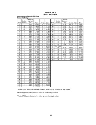
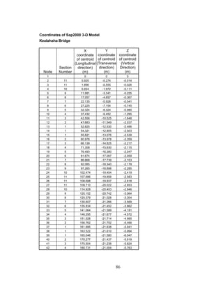
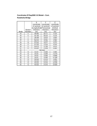
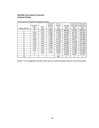
This document summarizes computer modeling of the proposed Kealakaha Stream Bridge replacement project in Hawaii. Finite element models of the bridge were created using SAP2000 and ANSYS software to analyze the bridge's behavior under various loads. A 2D and 3D frame model were made in SAP2000 and analyzed for modal frequencies and deformations from static truck loads. Additionally, a 3D solid model was made in ANSYS and analyzed for thermal loading effects, strains, modal frequencies, and deformations from static loads. The models provide predictions of the bridge's response that will be compared to sensor data collected from the actual bridge after construction.

1. Computer Modeling of the Proposed
Kealakaha Stream Bridge
Jennifer B.J. Chang
Ian N. Robertson
Research Report UHM/CEE/03-03
May 2003

3. ABSTRACT
The studies described in this report focus on the short-term structural performance
of a new replacement Kealakaha Bridge scheduled for construction in Fall 2003.
A new three span, 220-meter concrete bridge will be built to replace an existing
six span concrete bridge spanning the Kealakaha Stream on the island of Hawaii. During
and after construction, fiber optic strain gages, accelerometers, Linear Variable
Displacement Transducers (LVDTs) and other instrumentation will be installed to
monitor the structural response during ambient traffic and future seismic activity. This
will be the first seismic instrumentation of a major bridge structure in the State of Hawaii.
The studies reported here use computer modeling to predict bridge deformations
under thermal and static truck loading. Mode shapes and modal periods are also studied
to see how the bridge would react under seismic activity. Using SAP2000, a finite
element program, a 2-D bridge model was created to perform modal analysis, and study
vertical deformations due to static truck loads. A 3-D bridge model was also created in
SAP2000 to include the horizontal curve and vertical slope of the bridge. This model is
compared with the 2-D SAP2000 model to evaluate the effect of these and other
parameters on the structural response.
In addition, a 3-D Solid Finite Element Model was created using ANSYS to study
thermal loadings, longitudinal strains, modal analysis, and deformations. This model was
compared with the SAP2000 model and generally shows good agreement under static
truck loading and modal analysis. In addition, the 3-D ANSYS solid finite element model
gave reasonable predictions for the bridge under thermal loadings. These models will be
used as a reference for comparison with the measured response after the bridge is built.
iii

4. ACKNOWLEDGEMENTS
This report is based on a Masters Plan B report prepared by Jennifer Chang under
the direction of Ian Robertson. The authors wish to express their gratitude to Drs Si-
Hwan Park and Phillip Ooi for their effort in reviewing this report.
This project was funded by the Hawaii Department of Transportation (HDOT)
and the Federal Highway Administration (FHWA) program for Innovative Bridge
Research and Construction (IBRC) as part of the seismic instrumentation of the
Kealakaha Stream Bridge. This support is gratefully acknowledged. The content of this
report reflects the views of the authors, who are responsible for the facts and the accuracy
of the data presented herein. The contents do not necessarily reflect the official views or
policies of the State of Hawaii, Department of Transportation, or the Federal Highway
Administration. This report does not constitute a standard, specification or regulation.
iv

5. TABLE OF CONTENTS
Abstract…………………………………………………………………………. iii
Acknowledgements……………………………………………………………… iv
Table of Contents……………………………………………………………….. v
List of Tables……………………………………………………………….…… vii
List of Figures…………………………………………………………………… viii
Chapter 1 INTRODUCTION…..…………………………………………… 1
1.1 Project Description……………………………………………….. 1
1.2 Project Scope……………………………………………………… 5
Chapter 2 DESIGN CRITERIA FOR KEALAKAHA BRIDGE…………… 7
2.1 Geometric Data…………………………………………………… 7
2.2 Linear Soil Stiffness Data………………………………………… 7
2.3 Material Properties………………………………………………… 11
2.4 Boundary Conditions of Bridge…………………………………… 11
2.5 Bridge Cross Section……………………………………………… 11
Chapter 3 SAP2000 FRAME ELEMENT MODELS ……………………… 13
3.1 Development of SAP2000 Frame Element Models……………… 13
3.2 Element Sizes used for SAP2000 Models………………………… 16
3.3 Results of Frame Element Model Comparisons…………………… 18
3.3.1 Natural Frequencies…………………………………………18
3.3.2 Static Load Deformations………………………………….. 18
Chapter 4 ANSYS SOLID MODEL ………………………………………… 25
4.1 ANSYS Solid Model Development………………………………. 25
4.2 Finite Element Analysis: ANSYS, an Overview ..……………….. 26
4.3 Solid Model Geometry…………………………………………… 26
4.4 Development of Solid Model Geometry…………………………. 29
4.5 Meshing in ANSYS………………………………………………. 33
4.6 Test Beam: Determining Finite Element Type and Mesh for
Thermal Loading…………………………………………………. 34
4.7 Analytical Solution For Test Beam………………………………. 37
4.8 Comparison of ANSYS to Theoretical Result: Thermal Loading… 38
4.9 Comparison of ANSYS to Theoretical Result: Static Point Loading.39
4.10 Mesh Generation for Kealakaha Bridge Model……………………. 42
4.11 Convergence of 4 Meter Mesh…………………………………….. 42
Chapter 5 ANSYS SOLID MODEL ANALYSIS …………………………… 45
5.1 Truck Loading Conditions…………………………………………. 45
5.2 Truck Loading Results…………………………………………….. 46
5.2.1 Single 320 kN (72 Kip) Point Load……………………….. 46
5.2.2 Distributed Single Truck Load……………………………. 48
5.2.3 2x2 Truck Loading……………………………………….. 50
v

6. 5.2.4 4 Truck Loading Creating Torsion Effects………………… 52
Chapter 6 TEMPERATURE ANALYSIS …………………………………… 57
6.1 Temperature Gradient……………………………………………… 57
6.2 Results of Temperature Gradient………………………………….. 58
6.3 Strain Distribution…………………………………………………. 64
Chapter 7 MODAL ANALYSIS …………………………………………….. 67
7.1 Modal Periods……………………………………………………… 67
7.1.1 Modal Periods: 2-D vs. 3D Models…….…………………. 67
7.1.2 Modal Periods: Gross Section vs. Transformed Section….. 68
7.1.3 Modal Periods: Linear Soil Spring vs. Fixed Support….… 68
7.1.4 Modal Periods: SAP2000 vs. ANSYS….…………………. 69
7.2 Mode Shapes………………………………………………………. 70
Chapter 8 CONCLUSIONS AND SUMMARY……………………………… 79
8.1 Summary………………….………………………………………. 79
8.2 Conclusions……………………………………………………….. 79
8.3 Sources of Possible Error………………………………………….. 80
8.4 Suggestions for Further Study…………………………………….. 81
References …………………………………………………………………….. 83
Appendix A – Model Input Data ………………………………………………… 85
Coordinates of SAP2000 2-D Model …………………………………….. 85
Coordinates of SAP2000 3-D Model …………………………………….. 86
SAP2000 Cross Section Properties ………………………………………. 88
Material Properties used in SAP2000 ……………………………………. 89
ANSYS Solid Model – Coordinates ……………………………………… 90
ANSYS Solid Model – Cross-Section Depths …………………………… 91
vi

7. LIST OF TABLES
2.1 Kealakaha Bridge Geometric Data……………….……………………….. 7
2.2 Linear Soil Stiffness Data………………………………………………….. 8
3.1 Comparison of Vertical Deflections For Fixed Support…………………… 21
3.2 Comparison between Fixed Supports and Soil Springs ..…………………. 24
4.1 Vertical Deflection at Midspan on Test Beam: Thermal Loading………….39
4.2 Vertical Deflection at Midspan on Test Beam: 10 N Point Load…………. 41
4.3 Comparison between Four and Six Meter Mesh for ANSYS Model……… 44
5.1 Results of Single 320 kN Truck Point Load ….…………………………… 46
5.2 Vertical Deflection at Center of Bridge due to Single Truck
Load (Actual Wheels Modeled) .………………………………………….. 48
5.3 Vertical Deflection of Bridge due to 2x2 Truck Load
(Actual Wheels Modeled)………………………………………………….. 50
5.4 Vertical Deflection of Bridge due to 4 Truck Loading at Edge of Bridge
(Actual Wheels Modeled)…………………………………………………. 55
6.1 Vertical Deflection due to Temperature Gradient .……………………….. 62
7.1.1 Modal Periods: 2-D vs. 3D ……………………………………………… 67
7.1.2 Modal Periods: Gross Section vs. Transformed Section………………… 68
7.1.3 Modal Periods: Linear Soil Spring Support vs. Fixed Supports………… 69
7.1.4 Modal Periods: SAP2000 vs. ANSYS…………………………………… 69
vii

8. LIST OF FIGURES
1.1 Location of Project………………………………………………………… 1
1.2 Elevation, Section and Plan of Kealakaha Bridge ..….……………………. 2
1.3 UBC 1997 Seismic Zonation ..…………………….….…………………… 3
1.4 Horizontal Ground Acceleration (% g) at a 0.2 Second Period with 2%
Probability of Exceedance in 50 Years……………….……………………. 4
1.5 Horizontal Ground Accelerations (% g) at a 0.2 Second Period with 10%
Probability of Exceedance in 50 Years……………………………………. 5
2.1 Lateral Stiffness (Longitudinal Direction)……………………..………….. 9
2.2 Lateral Stiffness (Transverse Direction)………………………..…………. 9
2.3 Rotational Stiffness (Longitudinal Direction)…………………..…………. 10
2.4 Rotational Stiffness (Transverse Direction)……………………..………….10
2.5 Design Cross Section of Kealakaha Bridge…………………….………….. 12
3.1 SAP2000 2-D Frame Element Model (Schematic)………………………… 14
3.2 SAP2000 2-D Frame Element Model (Screen Capture)..………………….. 14
3.3 SAP2000 3-D Frame Element Model (Schematic)………………………… 15
3.4 SAP2000 3-D Frame Element Model (Screen Capture).………………….. 15
3.5 Element Lengths in SAP2000 Models……………………………..….…… 17
3.6 Convergence of Original and Half Size Finite Elements………….…….…. 18
3.7 Schematic Drawing of a Single HS20 Truck Load ………………..……… 19
3.8 Single HS20 Truck Load used in Chapter 3 ………………………..……... 19
3.9 Deformed Shape due to Single Truck Load ..……………………………… 20
3.10 Comparisons Between 2-D and 3-D Model .…………………………….... 21
3.11 Comparison of Gross and Transformed Section Properties for 2-D
Model Results ..……………………………………………………………. 22
3.12 Comparison of Gross and Transformed Section Properties for 3-D
Model Results …..…………………………………………………………. 22
3.13 Difference Between Fixed Support and Soil Springs: 2-D Model …..…… 23
3.14 Difference Between Fixed Support and Soil Springs: 3-D Model …...…… 24
4.1 Side View of a Portion of the Kealakaha Bridge……………………….…. 28
4.2.1 Design Cross Section………………………………………………….…… 30
4.2.2 Simplified Cross Section……………………………………………….….. 30
4.3 ANSYS Solid Model Cross Section View before Meshing…………….…. 31
4.4 Kealakaha Bridge before Meshing, Elevation ……………………………. 32
4.5 Kealakaha Bridge before Meshing, Isometric View………………………. 32
4.6 Solid 45, Eight Node Structural Solid (ANSYS) ….……………………… 34
4.7 Solid 92, Ten Node Tetrahedral Structural Solid (ANSYS) ..…………….. 34
4.8 Square Test Beam – Thermal Loading ……………………………………. 35
4.9 Thermal Distribution in Test Beam……………………………………….. 36
4.10 Test Beam Deflection under 10° C Temperature Gradient (Auto Mesh) … 38
4.11 Square Test Beam – Point Loading .………………………………………. 39
4.12 Four Meter Mesh Size, Kealakaha Bridge (Part of Bridge)……………….. 43
4.13 Six Meter Mesh Size, Kealakaha Bridge (Part of Bridge)…………………. 43
4.14 Convergence of Four and Six Meter Mesh for ANSYS Model …………… 44
5.1 Distribution of Truck Loads…………………………………….…………. 45
viii

9. 5.2 ANSYS Layout of Single Truck Point Load…………………………….… 47
5.3 SAP2000 vs. ANSYS, Single Truck Point Load…………………...……… 47
5.4 Viaduct Section Showing Single Truck Load………………………………48
5.5 Layout of Wheel Placement for Single Truck………………………..……. 49
5.6 SAP2000 vs. ANSYS, Single Truck Modeled with Wheels…………...….. 49
5.7 Location of Axle Loads for the 2x2 Truck Configuration ……………..…. 50
5.8 Viaduct Section showing 2x2 Truck Configuration……………………..… 51
5.9 ANSYS Placement of 2x2 Truck Load ………………….………………… 51
5.10 SAP2000 vs. ANSYS, 2x2 Trucks Modeled with Wheels……………….... 52
5.11 Location of Axle Loads for Four Trucks in a Row………………………....52
5.12 Viaduct Section showing Four Trucks in a Row…………………..………. 53
5.13 ANSYS Layout of Four Trucks in a Row………………………….……… 53
5.14 Deflected and Non-Deflected Cross Section……………………….……… 54
5.15 Torsion Effects, Four Trucks in a Row………………………………….… 54
5.16 Isometric View of Vertical Deflection under Torsion Loading………..….. 55
6.1 ANSYS Applied Temperature Gradient………………………………….... 57
6.2 Bridge End Span Showing Effect of Thermal Gradient……………….…... 58
6.3 Deformation due to 10 Degrees Temperature Gradient……………….…... 59
6.4 Isometric View of Bridge Deformation due to Thermal Loading……....…. 59
6.5 Side View of Bridge Deformation due to Thermal Loading………..…..…. 60
6.6 Locations of Reported Deformation due to Thermal Loading…...………... 61
6.7 Vertical Deflection of Bridge due to Ten Degree Temperature Gradient…. 62
6.8 Combination of Temperature and Truck Loading…………………………. 63
6.9 Strain Distribution through Box Girder Depth near Pier………………..… 64
6.10 Strain Distribution through Box Girder Depth near Midspan……………... 64
6.11 Strain Output Locations……………………………………………….…… 65
6.12 Longitudinal Strains at Locations A and B …………………………..…… 66
6.13 Longitudinal Strains at Locations C and D …………………………..……. 66
7.1 ANSYS Mode 2……………………………………………………….…… 70
7.2 SAP2000 Mode 1………………………………………………………..…. 70
7.3 ANSYS Mode 1………………………………………………………….… 71
7.4 SAP2000 Mode 2……………………………………………………….….. 71
7.5 ANSYS Mode 3……………………………………………………………. 72
7.6 SAP2000 Mode 3……………………………………….……………….…. 72
7.7 ANSYS Mode 4………………………………………….………………… 73
7.8 SAP2000 Mode 4………………………………………….…………….…. 73
7.9 ANSYS Mode 5…………………………………………….……………… 74
7.10 SAP2000 Mode 5…………………………………………….………….…. 74
7.11 ANSYS Mode 6……………………………………………….…………… 75
7.12 SAP2000 Mode 6………………………………………………………..…. 75
7.13 ANSYS Mode 7……………………………………………….…………… 76
7.14 SAP2000 Mode 7……………………………………………….……….…. 76
7.15 ANSYS Mode 8………………………………………………….………… 77
7.16 SAP2000 Mode 8………………………………………….…………….…. 77
7.17 ANSYS Mode 9………………………………………….………………… 78
7.18 SAP 2000 Mode 9……………………………………….……………….… 78
ix

10. x

11. CHAPTER 1
INTRODUCTION
1.1 Project Description
The project site is located along Mamalahoa Highway (Hawaii Belt Road) over
the Kealakaha stream in the District of Hamakua on the Island of Hawaii. The existing
bridge, a six span concrete bridge crossing the Kealakaha Stream is scheduled for
replacement in Fall 2003. The new replacement bridge will be built on the north side of
the existing bridge and will reduce the horizontal curve and increase the roadway width
of the existing bridge. The new bridge has been designed to withstand the anticipated
seismic activity whereas the existing bridge is seismically inadequate. Figure 1.1 shows
the location of the project on the Big Island of Hawaii.
Figure 1.1: Location of Project
1

12. The new prestressed concrete bridge will be a 3 span bridge and is approximately
220 meters long and 15 meters wide and will be designed to withstand earthquake and all
other anticipated loads. The new bridge will consist of three spans supported by two
intermediate piers and two abutments (Figure 1.2). The center span will be a cast-in-
place concrete segmental span of about 110 meters and the two outside spans will be
about 55 meters resulting in a balanced cantilever system. During and after construction,
fiber optic strain gages, accelerometers, Linear Variable Displacement Transducers
(LVDT’s) and other instrumentation will be installed to monitor the structural response
during ambient traffic and future seismic activity. This will be the first seismic
instrumentation of a major bridge structure in the State of Hawaii.
Figure 1.2: Elevation, Section and Plan of Kealakaha Bridge
2

13. The new bridge is in an ideal location for a seismic study because of the
earthquake activity on the island of Hawaii. The Island of Hawaii is in zone 4, the
highest zone of seismic activity categorized in the “1997 Uniform Building Code.”
Figure 1.3 shows the map of the “UBC 1997 Seismic Zonation” for the State of Hawaii.
Figure 1.3: UBC 1997 Seismic Zonation
Figures 1.4 and 1.5 show the peak ground acceleration maps included in the
International Building Code, IBC (2000). These maps are based on the USGS National
Seismic Hazard Mapping Project (USGS 1996). The maps show earthquake ground
motions that have a specified probability of being exceeded in 50 years. These ground
motion values are used for reference in construction design for earthquake resistance.
The maps show peak horizontal ground acceleration (PGA) at a 0.2 second period with
5% of critical damping. There are two probability levels: 2% (Fig. 1.4) and 10% (Fig.
1.5) probabilities of exceedence (PE) in 50 years. These correspond to return periods of
about 500 and 2500 years, respectively. The maps assume that the earthquake hazard is
independent of time.
3

14. The location of the Kealakaha bridge shows approximately 65% g with a 2%
probability of exceedance in 50 years (Fig. 1.4) and 35% g with a 10% probability of
exceedance in 50 years (Fig. 1.5). The acceleration due to gravity, g, is 980 cm/sec2.
Figure 1.4: Horizontal Ground Acceleration (%g) at a 0.2 Second Period With 2%
Probability of Exceedance in 50 Years (USGS, 1996)
4

15. Figure 1.5: Horizontal Ground Acceleration (%g) at a 0.2 Second Period With 10%
Probability of Exceedance in 50 Years (USGS 1996)
1.2 Project Scope
A number of computer models of the Kealakaha Bridge were created, analyzed
and compared to evaluate the structural response of the bridge to various loading
conditions. All models were linear elastic simulations in either SAP2000 (CSI 1997) or
ANSYS (ANSYS, 2002).
5

16. Frame element models were created in SAP2000 to determine the following:
1) Vertical deflection of the viaduct due to static truck loads.
2) Mode shapes and modal periods.
3) Effects of different degrees of modeling accuracy:
a. 3-D model compared with 2-D model.
b. Inclusion of linear soil stiffness properties (soil springs vs. fixed
supports.)
c. Inclusion of prestressing steel (transformed section vs. gross section
properties.)
d. Beam element size to produce convergence of results.
A three-dimensional solid model was created in ANSYS to determine the
following:
1) Deformation and strains of the viaduct due to thermal loads.
2) Deformation and strains of the viaduct due to truck loads.
3) Comparison of mode shapes and modal periods, and vertical deformations
under truck loads, with the SAP2000 frame element models.
6

17. CHAPTER 2
DESIGN CRITERIA FOR KEALAKAHA BRIDGE
The design specifications used for the Kealakaha bridge are the AASHTO LRFD
Bridge Design Specification – Second Edition (1998) including the 1999 and 2000
interim revisions (AASHTO, 1998). A geotechnical investigation was performed by
Geolabs, Inc. in 2001 and the report was available for this study (Geolabs, 2001a)..
Structural bridge data was obtained from Sato and Associates, the bridge design
engineers, and from the State of Hawaii project plans titled “Kealakaha Stream Bridge
Replacement, Federal Aid Project No. BR-019 2(26)” dated July 2001.
2.1 Geometric Data
The geometric data of the Kealakaha bridge are shown in Table 2.1. The bridge
radius and slopes were not modeled in the 2-D SAP2000 and the ANSYS models. The
bridge radius, longitudinal slope, and cross slope were included in the SAP2000 3-D
model.
Table 2.1: Kealakaha Bridge Geometric Data
Design Speed 80 km/hour
Span Lengths 55 m – 110 m – 55m
Typical Overall Structure Width 14.90 m (constant width)
Bridge Radius constant radius of 548.64 m
Bridge Deck constant cross slope of 6.2%
Vertical Longitudinal Slope Vertical curve changing to a constant
longitudinal slope of -3.46%
2.2 Linear Soil Stiffness Data
The only geotechnical information available for this study was the data provided
by Geolabs, Inc. in the project geotechnical report (Geolabs-Hawaii W.O. 3885-00
November 17, 1998). The study was done for Sato and Associates, Inc. and the State of
7

18. Hawaii Department of Transportation. The report summarized the findings and
geotechnical recommendations based on field exploration, laboratory testing, and
engineering analyses for the proposed bridge replacement project. The recommendations
were intended for the design of foundations, retaining structures, site grading and
pavements.
Geolabs, Inc. provided the design engineers with linear soil stiffness during
service conditions and extreme earthquake events using the secant modulus (Geolabs,
2001). A future proposed soil investigation and a soil-structure interaction-modeling
program will determine the non-linear and dynamic properties of the foundation material.
Figures 2.1 to 2.4 show plots of the secant modulus used to determine these linear
soil spring stiffness. Figure 2.1 shows the estimated secant modulus for lateral soil
stiffness in the bridge longitudinal direction with a lateral deflection of 0.0088 meters and
a lateral load of 18,750 kN. Figure 2.2 shows the secant modulus for the transverse
direction. The rotational stiffness in the bridge longitudinal direction was determined
from the secant modulus at a rotational displacement of 0.0054 rad and a moment of
165,000 kN-m (Figure 2.3). Figure 2.4 shows the secant modulus for the rotational
stiffness in the bridge transverse direction. These stiffness values are used for the soil
springs in the SAP2000 frame element models at the base of both piers. The values are
shown in Table 2.2.
Table 2.2: Linear Soil Stiffness Data
Lateral Stiffness
Longitudinal 2.12 X 106 kN/m
Transverse 1.89 X 106 kN/m
Rotational Stiffness
Longitudinal 3.29 X 108 kN-m/rad
Transverse 3.56 X 108 kN-m/rad
8

19. Lateral Stiffness (Longitudinal)
Calculating Secant Modulus
Data from Geolabs, Inc. 1/29/2001
20000
18000
16000
Lateral Load (kN)
14000 6
2.12X10 kN/m (Extreme Event)
12000
10000 6
2.9X10 kN/m (Service)
8000
6000
Fitted Curve
4000
2000 Secant Modulus
0
0 0.001 0.002 0.003 0.004 0.005 0.006 0.007 0.008 0.009 0.01
Lateral Deflection (meters)
Figure 2.1: Lateral Stiffness (Longitudinal Direction)
Lateral Stiffness (Transverse)
Calculating Secant Modulus
Data from Geolabs, Inc. 1/29/2001
20000 6
1.89X10 kN/m (Extreme Event)
18000
16000
Lateral Load (kN)
14000
12000
10000
8000
6000
4000
2000
Secant Modulus
0
0 0.001 0.002 0.003 0.004 0.005 0.006 0.007 0.008 0.009 0.01
Lateral Deflection (meters)
Figure 2.2: Lateral Stiffness (Transverse Direction)
9

20. Rotational Stiffness (Longitudinal)
Calculating Secant Modulus
Data from Geolabs, Inc. 1/29/2001
3.29X108 kN-m/rad (Extreme Event)
180000
160000
140000
Moment (kN-m)
120000
100000
80000
3.59X108 kN/m (Service)
60000
40000
20000 Fitted Curve
Secant Modulus
0
0 0.001 0.002 0.003 0.004 0.005 0.006
Rotation (Rad)
Figure 2.3: Rotational Stiffness (Longitudinal Direction)
Rotational Stiffness (Transverse)
Calculating Secant Modulus
Data from Geolabs, Inc. 1/29/2001
350000
8
3.56X10 kN-m/rad (Extreme Event)
300000
250000
Moment (kN-m)
200000
150000
100000
50000
Secant Modulus
0
0 0.0001 0.0002 0.0003 0.0004 0.0005 0.0006 0.0007 0.0008 0.0009 0.001
Rotation (Rad)
Figure 2.4: Rotational Stiffness (Transverse Direction)
10

21. 2.3 Material Properties
Based on the design documents obtained from Sato and Associates, three different
types of concrete were used to model the structure in the frame element models. Super-
structure concrete was used for the bridge span, sub-structure concrete was used for the
concrete piers and abutments, and weightless concrete was used for the dummy
connectors between the pier and the bridge girder in the SAP2000 frame element models.
Poisson’s ratio of 0.20 was used throughout the bridge. The Elastic Modulus was taken
as 2.4 x 107 kN/m2 for the bridge superstructure and 2.1 x 107 kN/m2 for the piers and
abutments.
2.4 Boundary Conditions of Bridge
For most computer models, the bases of the two piers were modeled as fully
fixed. In the SAP2000 soil spring model, rotational, horizontal, and vertical linear soil
springs were incorporated at the base of the piers. In all computer models, the abutments
at each end of the bridge were modeled as roller supports in the bridge longitudinal
direction, free to rotate about all axes, but restrained against vertical and transverse
displacement.
2.5 Bridge Cross Section
Figure 2.5 shows the design cross section of the Kealakaha bridge box girder.
From this cross section, centroidal coordinates, moments of inertia, torsion constants, and
cross-sectional areas were calculated for the SAP2000 models. All dimensions are
constant throughout the length of the bridge except the box girder depth, h, and the
bottom slab thickness, T. These values are listed in Appendix A for the end of each
bridge segment. The cross section in Figure 2.5 is referred to as the design cross section.
11

22. Modifications were made to simplify the cross-section for the ANSYS solid model as
explained in Chapter 4.
Figure 2.5: Design Cross Section of Kealakaha Bridge
12

23. CHAPTER 3
SAP2000 FRAME ELEMENT MODELS
3.1 Development of SAP2000 Frame Element Models
SAP2000 (CSI, 1997) was used to create the frame element models. Figures 3.1
and 3.2 show elevation, plan and isometric views of the 2-D model. This model ignores
the horizontal curve, longitudinal slope and cross slope. Note that although the roadway
is horizontal, the girder frame elements follow the centerline of the varying depth box
girder and are therefore curved in the vertical plane.
Figures 3.3 and 3.4 show elevation, plan and isometric 3-D views of the 3-D
model. In the 3-D model, the horizontal curve with radius of 548.64 m and the vertical
curve are modeled. The vertical curve begins as a varying slope until the center of the
bridge where it becomes a constant slope of –3.46 %. To model the bridge deck constant
cross slope of 6.2%, moments of inertia, and centerline coordinates were recalculated for
the 3-D model.
13

24. Figure 3.1: SAP2000 2-D Frame Element Model (Schematic)
Figure 3.2: SAP2000 2-D Frame Element Model (Screen Capture)
14

25. Figure 3.3: SAP2000 3-D Frame Element Model (Schematic)
Figure 3.4: SAP2000 3-D Frame Element Model (Screen Capture)
15

26. Eight frame element models were created based on these 2-D and 3-D geometries.
• 2-D frame element model (slopes and curve of bridge not considered)
1) Gross section properties neglecting the effect of prestressing steel
a) Fixed Supports
b) With linear soil springs at base of piers
2) Transformed section properties including prestressing steel
a) Fixed Supports
b) With linear soil springs at base of piers
• 3-D frame element model (slopes and curve of bridge included).
1) Gross section properties neglecting the effect of prestressing steel
a) Fixed Supports
b) With linear soil springs at base of piers
2) Transformed section properties including prestressing steel
a) Fixed Supports
b) With linear soil springs at base of piers
3.2 Element Sizes used for SAP2000 Models
To model the varying cross section along the length of the bridge, the box girder
was modeled using frame element segments. Each segment had the same section and
properties. The mass of each segment was computed automatically by SAP2000 based
the cross sectional area, concrete density, and frame element length.
The frame element size was based on the construction segment length throughout the
bridge. For the majority of the bridge length, 5.25 meter long elements were used. Three
1.5 meter long elements were used above each pier and abutment, and three 1 meter long
16

27. elements were used at the closure segment at the center of the middle span. Elements
used to model the piers varied in length from 1 m to 6.45 m. Figure 3.5 shows the
SAP2000 2-D model.
1m
1.5 m
5.25
Figure 3.5: Element Lengths in SAP2000 models
These element sizes were small enough to produce valid results. An analysis using finite
element sizes 50% smaller produced the same deflection results under a single truck
loading and the same modal frequencies. Figure 3.6 shows the results of the vertical
deflection under a single truck loading.
17

28. Sap2000 Frame Element Model
Vertical Deflection with Single Truck Loading at Center
Convergence of Original and Half Size Finite Elements
2 2-D No Steel Model
1
0
Vertical Deflection (mm)
0 50 100 150 200
-1
-2
-3
-4
-5
Original Size Elements
-6
Half Size Elements
-7
Along Length of Bridge (meters)
Figure 3.6: Convergence of Original and Half Size Finite Elements
3.3 Results of Frame Element Model Comparisons
3.3.1 Natural Frequencies
Natural frequencies, modal periods and mode shapes were determined for the first
nine modes for each of the eight SAP2000 frame element models. These results are
presented in Chapter six along with those from the ANSYS analysis.
3.3.2 Static Load Deformations
In order to evaluate the anticipated structural response to vehicle traffic, a number
of truck loading conditions were considered. This section presents the deflected shape
resulting from a single AASHTO HS20 truck located at midspan of the center span. This
loading condition is used to compare the various SAP2000 models. A single truck weighs
a total of 72 Kips or 320 kN. The truck scale dimensions are shown in Figure 3.7.
18

29. Figure 3.7: Schematic Drawing of a Single HS20 Truck Load
Chapter 4 shows results from modeling each axle or wheel for the HS20 loading
of Figure 3.7. In this section, a single point load of 320 kN is used to represent a single
truckload for comparisons of different computer modeling techniques as shown in Figure
3.8.
Figure 3.8: Single HS20 Truck Load Used in Chapter 3
19

30. Figure 3.9 shows the deflected shape of the bridge when subjected to a single
truck load at the center of the middle span using the 2-D SAP2000 model.
Figure 3.9: Deformed Shape due to Single Truck Load
20

31. Sap2000 Frame Element Model
Vertical Deflection with Single Truck loading at center of bridge
Fixed Foundation Support
Gross Section Properties
2
1
Vertical Deflection (mm)
0
0 50 100 150 200
-1
-2
-3
-4
-5 2-D
-6
3-D
-7
Along Length of Bridge (meters)
Figure 3.10: Comparison between 2-D and 3-D Models
Figure 3.10 shows that differences between the 2-D model and the 3-D model are
minimal for static deflections. At the center of the bridge, the maximum deflections
differ by only 0.07 mm between the 2-D and 3-D model as shown in Table 3.1.
Table 3.1: Comparison of Vertical Deflections For Fixed Support
Fixed Support 2-D Model 3-D Model Effect of Model
Models (mm) (mm) Type
Gross Section 5.92 5.85 0.07 (1.2 %)
Transformed
Section 5.139 5.07 0.07 ( 1.3 %)
Effect of
Prestressing Steel 0.78 (13.2 %) 0.78 (13.3 %)
(mm)
21

32. 2-D Sap2000 Frame Element Model
Vertical Deflection With Single Truck Loading at Center
Fixed Support Model With (Transformed) or Without (Gross) Prestressing
2 Steel
1
Vertical Deflection (mm)
0
0 50 100 150 200
-1
-2
-3
-4
2-D Model (Gross Section)
-5
-6 2-D Model (Transformed
Section)
-7
Along Length of Bridge (meters)
Figure 3.11: Comparison of Gross and Transformed Section Properties for 2-D
Model Results
3-D Sap2000 Frame Element Model
Vertical Deflection With Single Truck Loading at Center
Fixed Support Model With (Transformed) or Without (Gross) Prestressing
2
Steel
1
0
Vertical Deflection (mm)
0 50 100 150 200
-1
-2
-3
-4
3-D Model (Gross Section)
-5
-6 3-D Model (Transformed
Section)
-7
Along Length of Bridge (meters)
Figure 3.12: Comparison of Gross and Transformed Section Properties for 3-D
Model Results
22

33. When comparing the models with and without the prestressing steel, the
differences are more significant. Figures 3.11 and 3.12 show the comparison between
gross section and transformed section properties for the 2-D and 3-D models respectively.
Table 3.1 lists the maximum midspan deflections for each model showing differences of
0.78 mm (13.2%) and 0.78 mm (13.3%) for the 2-D and 3-D models respectively.
2-D Sap2000 Frame Element Model
Vertical Deflection with Single Truck Loading at Center of Bridge
2-D Models With or Without Linear Soil Spring
2
1
Vertical Deflection (mm)
0
0 50 100 150 200
-1
-2
-3
-4
-5 Gross Section Without Linear Soil
Springs
-6 Gross Section With Linear Soil
Springs
-7
Along Length of Bridge (meters)
Figure 3.13: Differences Between Fixed Supports and Soil Springs: 2-D Model
23

34. 3-D Sap2000 Frame Element Model
Vertical Deflection with Single Truck Loading at Center of Bridge
3-D Models With or Without Linear Soil Springs
2
1
Vertical Deflection (mm)
0
0 50 100 150 200
-1
-2
-3
-4
Gross Section Without Linear
-5 Soil Springs
-6 Gross Section With Linear Soil
Springs
-7
Along Length of Bridge (meters)
Figure 3.14: Difference Between Fixed Supports and Soil Springs: 3-D Model
Figures 3.13 and 3.14 show the differences between the fixed support and linear
soil springs used at the foundation of the piers for the 2-D and 3-D model respectively.
As stated previously, the soil springs are modeled with linear soil properties, and may not
accurately reflect actual soil response to different forces. Table 3.2 shows that there are
minimal differences in the vertical deflection between the fixed and spring foundation
and minimal differences between the 2-D and 3-D model. For this reason, and to keep the
ANSYS solid model under 32,000 nodes, the solid model was generated as a straight
model (equivalent to the SAP2000 2-D fixed geometry) using fixed supports at the piers.
Table 3.2: Comparison between Fixed Supports and Soil Springs
2-D Model 3-D Model Effect of Model
(mm) (mm) Type
Linear Soil Spring 5.98 5.92 0.06 (1%)
Fixed Foundation 0.07 (1.2%)
5.92 5.85
Effect of Soil
Springs 0.06 (1%) 0.07 (1%)
24

35. CHAPTER 4
ANSYS SOLID MODEL
4.1 ANSYS Solid Model Development
Reasons for creating a solid model in ANSYS include:
• More detailed representation than a frame element model
• Output strain values for use in designing a strain-based deflection system
• Study torsion effects of eccentric truck loads
• Predict thermal deformations
• ANSYS has nonlinear modeling capabilities for use in future seismic analysis.
Several software programs were considered for analyzing the solid model.
• Sap 2000 Version 8 (CSI 2002)
• ANSYS Version 6.1 (ANSYS Inc, 2002)
• Abaqus-Standard Version 6.0 (Abaqus, Inc. 2002)
• I-deas
ANSYS was the choice of software for creating the solid model. SAP2000 did not have
the capability of creating a box girder bridge with a varying cross section. SAP2000 did
not have adequate meshing capabilities and could only mesh solid models in linear
elements. I-deas was used previously to create solid bridge models of the H-3 (Ao 1999)
but the College of Engineering at the University of Hawaii no longer has a license for
I-deas. Between Abaqus and ANSYS, ANSYS appeared to be the more “user friendly”
software with a simple tutorial and CAD input capabilities.
25

36. 4.2 Finite Element Analysis: ANSYS, an Overview
ANSYS is a finite element analysis program used for solid modeling. It has
extensive capabilities in thermal, and structural analysis.
The solid model consists of key points/nodes, lines, areas and volumes with
increasing complexity in that order. Careful thought needs to be put into the model
before building the entire model. Once the model is meshed, volumes, areas, or lines
cannot be deleted if they are connected to existing meshed elements. The aspect ratio and
type of mesh must also be decided depending on the size and shape of the complete solid
model.
ANSYS contains many solid finite elements to choose from, each having its own
specialty. First, the type of analysis must be chosen which ranges from structural
analysis, thermal analysis, or fluid analysis. Once the type of analysis is determined, an
element type needs to be chosen ranging from beam, plate, shell, 2-D solid, 3-D solid,
contact, couple-field, specialty, and explicit dynamics. Each element has unique
capabilities and consists of tetrahedral, triangle, brick, 10 node, or 20 node finite
elements both in 2-D or 3-D analysis.
4.3 Solid Model Geometry
There are three ways to create a model in any finite element program for solid modeling.
1) Direct (manual) generation
• Specify the location of nodes
• Define which nodes make up an element
• Used for simple problems that can be modeled with line elements
(links, beams, pipes)
26

37. • For objects made of simple geometry (rectangles)
• Not recommended for complex solid structures
2) Importing Geometry
• Geometry created in a CAD system like Autodesk Inventor
• Saved as an import file such as an IGES file.
• Inaccuracies occur during the import, and the model may not
import correctly.
3) Solid Modeling Approach
• The model is created from simple primitives (rectangles, circles,
polygons, blocks, cylinders, etc.)
• Boolean operations are used to combine primitives.
Direct manual generation was the approach used to create the SAP2000 frame
element models. However when creating a solid model that contains over 20,000 nodes,
this approach is not recommended.
Using a CAD program such as Autodesk Inventor to create the solid model was
also investigated. Autodesk Inventor had a very good CAD capability compared to
creating the model in the ANSYS CAD environment. However, attempts to import the
IGES file into ANSYS were unsuccessful. The model did not import correctly due to
software incompatibility.
The solid modeling approach was used to create the Kealakaha Bridge. Creating
the top slab of the bridge with the “extrude” command was easy because it was the same
shape throughout the bridge. However, when creating the box girder, the cross section
varied throughout the length of the bridge. ANSYS did not have good CAD capabilities
27

38. to create many volumes in 3-D space with a varying cross section. When creating the
solid volume for the box girder, each solid element had to be created using only 8 nodes
at a time by using the “create volumes arbitrary by nodes” command. Creation of the
final bridge model was accomplished by dividing the bridge into many volumes and
combining them together. Figure 4.1 shows the side view of portion of the bridge. Each
color represents a different area and block volume that had to be created and joined
together using the Boolean operation. Due to symmetry, the reflect and copy command
was used to create the other half of the bridge.
1
AREAS
FEB 19 2003
AREA NUM 11:00:21
Y
Z X
Figure 4.1: Side View of a Portion of the Kealakaha Bridge
28

39. 4.4 Development of Solid Model Geometry
The program that was used to analyze the solid model was ANSYS/University
High Option, Version 6.1. Limitations to this software include the maximum number of
nodes which is set at 32,000 nodes. To keep the number of nodes below this limit, the
original cross section could not be used without having a large aspect ratio during
meshing. To reduce the amount of nodes as well as computation time, the cross section
model had to be simplified. Weng Ao (1999) performed a similar study on the North
Halawa Valley Viaduct (NHVV), which is part of the H-3 freeway. The NHVV box
girder shape was very similar to the Kealakaha bridge box girder. Ao used simpler cross
sections than the original box girder and compared the predicted to measured results.
Even with simplification of the cross sections, the analytical results using the I-deas solid
modeling program showed good agreement with actual results for both thermal and truck
loading conditions.
The simplified cross section shown in Figure 4.2.2 was created by averaging the
top and bottom slab thickness of the design cross section to create an equivalent area in
the simplified cross section. The moment of inertia was changed by no more than 3% in
the lateral direction and 11% in the vertical direction.
Figure 4.2.1 shows the design cross section that was used to compute section properties
for the frame element models in SAP2000. Figure 4.2.2 shows the simplified cross
section used for the solid model in ANSYS. The depths and heights that vary are listed in
the Appendix.
29

40. Figure 4.2.1: Design Cross Section
Figure 4.2.2 Simplified Cross Section
30

41. 1
VOLUMES
FEB 19 2003
TYPE NUM 11:02:06
Y
Z X
Figure 4.3: ANSYS Solid Model Cross Section before Meshing
Figure 4.3 shows a close up view of the simplified cross section in ANSYS. Figures 4.4
and 4.5 show the completed solid model before meshing. The piers have fixed supports
while the abutment ends are restrained against vertical and lateral movement
perpendicular to the bridge.
31

42. 1
VOLUMES
FEB 20 2003
TYPE NUM 11:27:15
U
Y
Z X
Figure 4.4: Kealakaha Bridge before Meshing, Elevation
1
VOLUMES
FEB 20 2003
TYPE NUM 11:26:02
U
Y
Z X
Figure 4.5: Kealakaha Bridge before Meshing, Isometric View
32

43. 4.5 Meshing in ANSYS
Meshing in ANSYS can be applied manually or automatically. The element type
selected (Linear vs. Tetrahedral), and the mesh size can affect the accuracy of the results
of the analysis. Due to the large model size, automatic meshing was not possible for the
entire Kealakaha bridge. In automatic meshing, ANSYS automatically chooses a
meshing size based on the shape of the model. This resulted in more elements than
permitted by the University High Option of ANSYS. Manual meshing allows the user to
define the maximum size of the elements.
To guide the selection of element type, a test beam was created in ANSYS to
determine what solid finite element produced the best results for deflection under thermal
loading. There are two types of elements in ANSYS that have both structural and
thermal capabilities for solid modeling. They are Solid 45 which is an eight node brick
(cube shaped) element (Fig. 4.6) and Solid 92 which is a 10 node tetrahedral element
(Fig. 4.7). These elements were tested under thermal and static loads on a test beam to
determine which element produced the best results when compared to the theoretical
values.
33

44. Figure 4.6: Solid 45, Eight Node Structural Solid (ANSYS)
Figure 4.7: Solid 92, Ten Node Tetrahedral Structural Solid (ANSYS)
4.6 Test Beam: Determining Finite Element Type and Mesh for Thermal Loading
Solid 45 and Solid 92 were evaluated using a test beam that was 10 meters long
by one meter thick and one meter high. The sample test beam was also created to test the
performance of ANSYS under thermal loading conditions. Simply supported end
conditions were used for the test beam as shown in Figure 4.8.
34

45. 10 Degrees
10 m
1m
Temp
Gradient
Figure 4.8: Square Test Beam-Thermal Loading
A 10-degree temperature gradient was produced by applying two different
temperatures at the top and bottom surfaces of the beam. A temperature gradient is
anticipated for the top slab of the Kealakaha bridge during solar heating similar to the H-
3 study (Ao 1999). The thermal expansion coefficient was arbitrarily chosen as 10-5 per
degrees Celsius for this test beam. Figure 4.9 shows the distribution of the temperature
that was applied throughout the beam. The red indicates a temperature of 10 degrees C,
while the blue represents a temperature of 0 degrees C. The actual thermal expansion
coefficient used in the Kealakaha bridge model will be based on concrete cylinder tests
and is expected to be in the range of 10 to 11X10-5 per degree Celsius. For the thermal
analysis performed in this study, a value of 11X10-5 per degree Celsius was used for the
Kealakaha bridge model. Concrete properties similar to the top slab of the Kealakaha
bridge was used for the test beam.
35

46. 1
NODAL SOLUTION
FEB 19 2003
STEP=1 11:33:04
SUB =1
TIME=1
BFETEMP (AVG)
RSYS=0
DMX =.001304
SMX =10 Y
MX
Z X
MN
0 2.222 4.444 6.667 8.889
1.111 3.333 5.556 7.778 10
Figure 4.9: Thermal Distribution in Test Beam
36

47. 4.7 Analytical Solution For Test Beam
The deformation due to a linear temperature change can be expressed as:
d dv α∆T
=
dx dx h
where v = Vertical Deflection
α = Coefficient of Thermal Expansion
= 10-5/°C in the test beam
∆T = Change in temperature between top and bottom surfaces
= 10 °C in the test beam
h = Depth of the beam
= 1 meter in the test beam
Therefore,
dv α∆T x + A
=
dx h
1 α∆T 2
v= x + Ax + B
2 h
where A and B are integration constants.
Applying boundary conditions: At x=0, v(0)=0 and at x=10, v(10)=0 and substituting the
numerical values into the equation, we obtain:
v = (50-5x)x*10-5
At the midspan, x = 5 meters therefore:
v = 0.00125 meters
There should be a maximum deflection of 0.00125 meters at the center of the test beam.
37

48. Figure 4.10 shows the deflection result of the test beam in ANSYS due to the 10 degrees
temperature gradient using the solid 92 element. The automatic meshing tool was used
which produced element sizes close to 0.5 meters.
1
DISPLACEMENT
FEB 19 2003
STEP=1 11:32:31
SUB =1
TIME=1
DMX =.001304
Y
Z X
Figure 4.10: Test beam deflection under 10° Celcius Temperature Gradient
(Automatic Mesh)
4.8 Comparison of ANSYS to Theoretical Result: Thermal Loading
Table 4.1 shows the comparison between Solid 45 and Solid 92 for the thermal
loading conditions. Varying the element size from 0.25 to 1 meter had very little effect
on the vertical deflection under thermal loading. The theoretical result is 1.25 mm for the
vertical deflection at midspan. The percentage error in Table 4.1 is the error compared to
the theoretical result.
38

49. Table 4.1: Vertical Deflection at Midspan on Test Beam: Thermal Loading
Vertical Deflection at Percentage Error
Midspan (mm)
Theoretical Result 1.25 -
Solid45 1.128 9.8%
Eight Node Structural Solid
(Brick Node)
Solid 92 1.304 4.3%
Ten Node Structural Solid
Tetrahedral Shaped
Solid 92 gave the lowest percentage error of 4.3% when compared with the analytical
result.
4.9 Comparison of ANSYS to Theoretical Result: Static Point Loading
A static point load of 10 Newton applied to the midspan of the test beam
using different element types and sizes as shown in Figure 4.11.
10 N (at midspan of beam)
1m
10 m
Figure 4.11: Square Test Beam – Point Loading
39

50. For a simply supported beam under a midspan point load, the theoretical deflection is:
Vertical Deflection ∆ = − PL
3
48 EI
where P = Load at midspan
= 10 N on test beam
L = Length of beam
= 10 m for test beam
E = Modulus of Elasticity
= 2.4X107 kN/m2 for test beam
= Moment of Inertia = bh
3
I
12
= 1 m4for test beam
12
Substituting the numerical values produces the following theoretical result:
∆ = 1.041X10-7 m down
Table 4.2 lists the comparisons between the Solid 45 and Solid 92 elements for
the vertical deflection at the midspan due to a 10 N point load. The theoretical result will
not match the result from ANSYS because the theoretical result does not include shear
deformation. However, the % difference between the theoretical and ANSYS will be
used. The results show that Solid 92 consistently predicted deflections close to the
theoretical result with the percent difference ranging from 3.2 to 5.4%. The solid 45
results range from 5.76 to 62 percent and are highly dependant on the mesh element size.
For this reason, Solid 92 would be the better choice under a static load.
40

51. Table 4.2: Vertical Deflection at Midspan on Test Beam: 10 N Point Load
Solid45 Solid 92
Element Size Eight Node Structural Solid Ten Node Structural Solid
(Brick Node) Tetrahedral Shaped
Vertical % Vertical %
Deflection at Difference Deflection at Difference
Midspan From Midspan From
-7 -7
(X10 m) Theoretical (X10 m) Theoretical
Automatic Meshing 1.128 8.3 1.09 4.7
0.25 meters 1.178 13.2 1.08 3.7
0.5 meters 0.961 7.7 1.09 4.7
1 meter 0.472 55 1.1 5.6
Theoretical Result 1.041 X10-7m 1.041 X10-7m
Structural Solid 92 was selected for meshing the Kealakaha Bridge model.
Solid 92 has a quadratic displacement behavior and is well suited to model irregular
geometries as shown in Figure 4.7. The element can model plasticity, creep, swelling,
stress stiffening, large deflection, and large strain conditions.
When applying a thermal load, a thermal solid element must also be selected.
ANSYS automatically chose Thermal Solid 87 for both test beam and bridge models.
Thermal analysis is done separately in ANSYS, and is saved as a .rth file in the working
directory. In thermal analysis, one must transfer the element type from a structural
element to thermal element so that thermal loads can be applied linearly. This is
important because if the program is in structural element mode, the temperatures will
only be applied at the surface of the beam, and will not be applied linearly throughout the
entire beam. After running the thermal analysis, the .rth file must be imported into the
structural element mode with Solid 92 and applied as a “temperature from thermal
analysis.” After running the structural analysis, structural deformation/stress/strain results
are produced.
41

52. 4.10 Mesh Generation for Kealakaha Bridge Model
ANSYS has the capability of doing automatic meshing where it automatically
picks an element size. However, automatic meshing may not produce the best results and
cannot be used for the 220 meter Kealakaha bridge because it will produce over 32,000
nodes which exceeds the University program capability. The “mesh tool” command must
be used to specify the element size.
Based on the specified element size, ANSYS will mesh the model to produce the
best results. The element size will not be the same for all elements, but all elements will
be smaller than the specified size.
The mesh size used for the Kealakaha bridge was 4 meters. A similar mesh size
of 12 feet was used in the NHVV study by Weng Ao (1999), and produced good results
when compared with measured deflections. Figure 4.12 shows the 4 meter mesh for a
portion of the bridge. The full bridge consisted of 24,576 nodes and 12,246 elements.
4.11 Convergence of 4 Meter Mesh
To confirm that the four-meter mesh converges with a larger size mesh, a six
meter mesh was created and the response to a single truck load was compared. See
Figure 3.8 for a description of the single truck load. The four-meter mesh is seen in
Figure 4.12 and the six-meter mesh is shown in Figure 4.13.
42

53. 1
ELEMENTS
FEB 20 2003
11:14:11
Figure 4.12: Four Meter Mesh Size, Kealakaha Bridge (Part of Bridge)
1
ELEMENTS
Figure 4.13: Six Meter Mesh Size, Kealakaha Bridge (Part of Bridge)
43

54. ANSYS Solid Model
Vertical Deflection with Single Truck loading at center of bridge
Convergence of Four Meter Mesh Vs. Six Meter Mesh
2
1
Vertical Deflection (mm)
0
0 50 100 150 200
-1
-2
-3
-4
-5 4 Meter Mesh
-6
6 Meter Mesh
-7
Distance Along Bridge (meters)
Figure 4.14: Convergence of Four and Six Meter Mesh for ANSYS Model
Table 4.3: Comparison between Four and Six Meter Mesh for ANSYS Model
Six Meter Mesh Four Meter Mesh Difference (%)
Vertical Vertical Deflection
Deflection (mm) (mm)
Maximum End 0.94 0.96 0.02 (2.1%)
Span Deflection
Maximum Center -5.73 -5.73 0 (0%)
Span Deflection
The results plotted in Figure 4.14 show convergence between a four meter mesh
and a six meter mesh. The results at the maximum deflection for the end span and center
span under a single truck loading are shown in Table 4.3. In Table 4.3, there is a 0%
difference in the center span deflection, and only a 2.1% difference in the end span
deflection. Therefore, a four-meter mesh is adequate for this analysis.
44

55. CHAPTER 5
ANSYS SOLID MODEL ANALYSIS
5.1 Truck Loading Conditions
According to the design criteria on the construction plans, a typical truck weighs a
total of 320 kN or 72 Kips with the dimensions shown in Figure 5.1.
Figure 5.1: Distribution of Truck Loads
Each 320 kN truck has six wheels and the load is divided among all six wheels for
the ANSYS solid model. The total axle load shown in Figure 5.1 is divided by two to get
the load for each wheel. In ANSYS, loads can only be applied to existing nodes
produced by the mesh. The mesh size used was 4 meters, so the loads were placed at the
closest possible node to produce the actual wheel location.
Three different truck-loading conditions were considered in this analysis. In all of
these analyses, the truck placement was symmetrical about the midspan of the center span
of the bridge. The three loading conditions are:
45

56. • Single Truck Load on centerline of roadway
• Four Trucks (Two rows of two trucks each, 2x2 Truck Load) on centerline
of roadway
• Four Trucks (All four trucks in a single line) at edge of roadway
In ANSYS, each wheel was modeled as a load, however in the SAP2000 frame
element analysis, each axle was modeled as a load. ANSYS and SAP2000 model results
are compared in the following sections.
In addition, the SAP2000 frame element model and the ANSYS solid model were
also compared when a single 320 kN point load was applied at the center of the roadway
at midspan of the center span.
5.2 Truck Loading Results
5.2.1 Single 320 kN (72 Kip) Point Load
Figure 5.2 shows the single 320 kN truck point load applied to the top slab of the
ANSYS model. Figure 5.3 shows a comparison between SAP2000 and ANSYS while
Table 5.1 shows the vertical displacement under the 320 kN point load.
The maximum deflection from the SAP2000 model is less than the ANSYS
model, but at all other nodes the ANSYS model yielded slightly less deflections. The
local deformation of the top slab under the single concentrated load does not correctly
represent the effect of the truck loading.
Table 5.1: Results of Single 320 kN Truck Point Load
Sap2000 ANSYS Difference
Single Truck Load Single Truck Load
Vertical Deflection at 0.4
Center of Bridge Span (mm) -5.92 -6.32 (6.7%)
Maximum End Span 0.03
Deflection (mm) 1.04 1.01 (2.9%)
46

57. 1 2
ELEMENTS ELEMENTS
U U
F F
Z Y
X
3
ELEMENTS
U
F
Y
Z X
Figure 5.2: ANSYS Layout of Single Truck Point Load
SAP2000 Vs. ANSYS
Single Truck (Point Load) at Center of Bridge
2
1
Vertical Deflection (mm)
0
0 50 100 150 200
-1
-2
-3
-4
-5 ANSYS
-6
SAP2000
-7
Along Length of Bridge (meters)
Figure 5.3: SAP2000 vs. ANSYS, Single Truck Point Load
47

58. 5.2.2 Distributed Single Truck Load
Figure 5.4 shows the viaduct section with a single truck loading placed at the
center of the section and at the center span along the length of the bridge. Isometric, top
and side views are shown in ANSYS in Figure 5.5. The results for the vertical deflection
due to the single truck load are shown in Figure 5.6. Wheels were modeled to conform to
Figure 5.1 but dimensions of the truck wheels vary according to the node locations in the
solid model. The results for deflections are shown in table 5.2
Table 5.2: Vertical Deflection at Center of Bridge due to Single Truck Load, Actual
Wheels Modeled
Vertical Deflection at Center of
Bridge (mm)
SAP2000 Each ANSYS Difference
Axle Modeled Each Wheel (mm)
Modeled
Vertical Deflection at Center
of Bridge Span (mm) -5.69 -5.73 0.04 mm (0.6%)
Maximum End Span
Deflection (mm) 0.98 0.97 0.2 mm (3.2%)
Figure 5.4 Viaduct Section Showing Single Truck Load
48

59. 1 2
ELEMENTS ELEMENTS
U U
F 5.25 m F
10.38 m
Z Y
X
3
ELEMENTS
U
F
Y
Z X
3.12 m
Figure 5.5: Layout of Wheel Placement for Single Truck
SAP2000 Vs. Ansys
Single Truck Load at Center Of Bridge
ANSYS: Each Wheel Modeled
SAP2000: Each Axle Modeled
2
1
Vertical Deflection (mm)
0
0 50 100 150 200
-1
-2
-3
-4
-5 ANSYS
-6
SAP2000
-7
Along Length of Bridge (meters)
Figure 5.6: SAP2000 vs. Ansys, Single Truck Modeled with Wheels
49

60. 5.2.3 2x2 Truck Loading
Figure 5.7 shows the locations of the axles for the 2x2 truck loading. Figure 5.8
shows the viaduct section under the 2x2 truck loading. The trucks are placed
symmetrically about the center span to reduce computational time for the analysis and
produce symmetrical deflected shapes. The axle spacing is larger than as shown in
Figure 5.1 due to limited node locations available for applying the loads. Figure 5.9
shows the layout of the 2x2 truck loading in ANSYS. The vertical deflection results are
shown in Figure 5.10 and Table 5.3.
Table 5.3: Vertical Deflection of Bridge Due to 2x2 Truck Load
(Actual Wheels Modeled)
Vertical Deflection at Center of
Bridge (mm)
SAP2000 Each ANSYS Difference
Axle Modeled Each Wheel (mm)
Modeled
Vertical Deflection at
Center of Bridge Span -19.49 -19.17 0.32 mm (1.6%)
(mm)
Maximum End Span
Deflection 3.77 3.61 0.16 mm (4.2%)
(mm)
Midspan of Bridge Center Span
Figure 5.7: Location of Axle Loads for the 2x2 Truck Configuration
50

61. Figure 5.8: Viaduct Section showing 2x2 Truck Configuration
1 2
ELEMENTS ELEMENTS
U U
F F
Z Y
X
3
ELEMENTS
U
F
Y
Z X
Figure 5.9: ANSYS Placement of 2x2 Truck Load
51

62. SAP2000 Vs ANSYS
2X2 Truck Load, 4 Trucks Total
ANSYS: Each Wheel Modeled
SAP2000: Each Axle Modeled
5
0
Vertical Deflection (mm)
0 50 100 150 200
-5
-10
-15
ANSYS
-20
SAP2000
-25
Length Along Bridge (meters)
Figure 5.10: SAP2000 vs. ANSYS, 2x2 Truck Modeled with Wheels
5.2.4 4 Truck Loading Creating Torsion Effects.
4 truck loads were placed at the edge of the viaduct cross section to study torsion
effects due to eccentric loading. Figure 5.11 shows the locations of the axle loadings for
the trucks. The trucks are placed symmetrically about the center span of the bridge to
reduce the computational time for the analysis and to generate a symmetrical deflected
shape.
Midspan of bridge center span
Figure 5.11: Location of Axle Loads for Four Trucks in a Row
52

63. The 4 trucks modeled at the right edge of the viaduct section are shown in Figure
5.12. Figure 5.12 show the locations “A,” “B,” and “C,” where the vertical deflections
were recorded. Location “C” is at the middle of the cross section. Location “B” is on the
side of the truck loading above the box girder stem and location “A” is on the opposite
side above the box girder stem. Figure 5.13 shows the layout of the 4 trucks in ANSYS.
The loads are applied at the nodes.
Figure 5.12: Viaduct Section showing Four Trucks in a Row
1 2
ELEMENTS ELEMENTS
U U
F F
Z Y
X
3
ELEMENTS
U
F
Y
Z X
Figure 5.13: ANSYS Layout of Four Trucks in a Row
53

64. Figure 5.14 shows the deflected and non-deflected shape of the cross section modeled in
ANSYS at midspan of the center span of the bridge, the legend at the bottom shows the
vertical deflection in meters. Locations “A,” “B,” and “C” are shown at the top of the
slab (See Figure 5.12 for more precise locations). The result of the vertical deflection
due to the truck load are shown in Figure 5.15.
1
Truck
Y
Z X
A
C
B
-.02163 -.015896 -.010162 -.004427 .001307
-.018763 -.013029 -.007295 -.00156 .004174
Figure 5.14: Deflected and Non-Deflected Cross Section
ANSYS: Torsion Effects
4 Trucks in a Row at Edge of Bridge
ANSYS: Each Wheel Represented By One Load
5
0
Vertical Deflection (mm)
0 50 100 150 200
-5
-10 Location A
Location B
-15
Location C
(Center)
-20
Along Length of Bridge (meters)
Figure 5.15: Torsion Effects, Four Trucks in a Row
54

65. Table 5.4 shows the results of the vertical deflections at locations “A,” “B,” and
“C.” The torsion effect shows that there is a 2.43 mm difference between the left and
right sides of the bridge cross section at the center span and a 0.57 mm difference in the
maximum end span deflections.
Table 5.4: Vertical Deflection of Bridge due to 4 Truck Loading at Edge of Bridge
(Actual Wheels Modeled)
Vertical Deflection in Cross
Section Points A and B (mm)
ANSYS ANSYS % Difference
Location A Location B (torsion effect)
(Left) (Right)
Vertical Deflection at Center
of Bridge Span (mm) -16.20 -18.63 2.43 (13.0%)
Maximum End Span
Deflection (mm) 3.71 3.14 0.57 (15.4%)
Figure 5.16 shows an isometric view of the bridge with color contours for the
vertical deflection of the bridge. The torsion effect can be seen by the different colors.
The legend shows the deflection in meters.
1
NODAL SOLUTION
STEP=1
SUB =1
TIME=1
UY (AVG)
RSYS=0 MX
DMX =.021714
SMN =-.02163
SMX =.004174
MN
Y
Z X
-.02163 -.015896 -.010162 -.004427 .001307
-.018763 -.013029 -.007295 -.00156 .004174
Figure 5.16: Isometric View of Vertical Deflection under Torsion Loading
55

66. 56

67. CHAPTER 6
TEMPERATURE ANALYSIS
6.1 Temperature Gradient
Figure 6.1: ANSYS Applied Temperature Gradient
Figure 6.1 show the temperature gradient applied to the ANSYS solid model. A
10 degrees Celsius linear temperature gradient is applied through the 0.35 m thick top
slab. The temperature gradient was based on temperature measurements from the NHVV
(Ao, 1999). Below the top slab, the temperature was assumed constant at zero degrees
throughout the box girder, and piers. This thermal loading develops by mid afternoon
due to solar radiation on the top surface of the bridge. Thermocouples will be installed in
the Kealakaha Bridge to record the exact temperature gradients after the bridge is built.
The coefficient of thermal expansion used for this analysis was 11X10-5 per
degrees Celsius.
57

68. 1
NODAL SOLUTION
STEP=1
SUB =1
TIME=1
BFETEMP (AVG)
RSYS=0
DMX =.008688
SMX =10
MX
0 2.222 4.444 6.667 8.889
1.111 3.333 5.556 7.778 10
Figure 6.2: Bridge End Span Showing Effect of Thermal Gradient
6.2 Results of Temperature Gradient
Figure 6.2 shows the temperature gradient applied through the top slab of the
bridge and the resulting exaggerated deformed shape. Figure 6.3 shows the deformation
of the bridge due to the 10 degree temperature gradient. Figures 6.4 and 6.5 show
isometric and side views of the deformation of the bridge.
58

69. 1 2
DISPLACEMENT DISPLACEMENT
STEP=1 STEP=1
SUB =1 SUB =1
TIME=1 TIME=1
DMX =.008688 DMX =.008688
Z Y
Y X
Z X
3 4
DISPLACEMENT DISPLACEMENT
STEP=1 STEP=1 Y
SUB =1 SUB =1
TIME=1 TIME=1 Z X
DMX =.008688 DMX =.008688
Y
Z X
Figure 6.3: Deformation due to 10 Degree Temperature Gradient
1
DISPLACEMENT
STEP=1
SUB =1
TIME=1
DMX =.008688
Y
Z X
Figure 6.4: Isometric View of Bridge Deformation due to Thermal Loading
59

70. 1
DISPLACEMENT
STEP=1
SUB =1
TIME=1
DMX =.008688
Y
X Z
Figure 6.5: Side View of Bridge Deformation due to Thermal Loading
60

71. The deflected shape is plotted along the middle of the top slab (location “a”),
along the top of the box stems (“b”) and along the edge of the top slab cantilevers (“c”).
Locations “a” and “c” are affected by longitudinal and transverse deformations as seen in
Figure 6.5, hence location “b,” above the box girder stems, is assumed to be the best
representation of the deformed shape of the bridge spans. Comparisons with measured
deflections based on the field instrumentation will confirm whether these predicted
deflections are accurate.
Figure 6.6 shows the approximate locations “a,” “b,” and “c” in the cross section
view indicated by the circles.
a
b b
Y
Z X
c
c
-.008667 -.006269 -.003872 -.001475 .922E-03
-.007468 -.005071 -.002674 -.276E-03 .002121
Figure 6.6: Locations of Reported Deformation due to Thermal Loading
61

72. ANSYS Solid Model
Vertical Deflection due to Gradient Temperature of 10 Degrees Celcius through top
slab
4
Deflection along roadway centerline (a)
2 Deflection above base stems (b)
Deflection at end of cantilever (c)
Vertical Deflection (mm)
0
0 50 100 150 200
-2
-4
-6
-8
-10
Distance Along Bridge (meters)
Figure 6.7: Vertical Deflection of Bridge due to Ten Degree Temperature Gradient
Table 6.1: Vertical Deflection due to Temperature Gradient
Deflection (mm) Deflection Deflection
Along Roadway (mm) Above (mm) at End of
Distance Along Centerline Base Stems Cantilever
Bridge (meters) “a” “b” “c”
16.75 m and 2.1 1.79 1.19
203.25 m
110 m -5.08 -5.48 -8.66
Figure 6.7 shows the vertical deflections at points a, b, and c. The results at the
center span and maximum deflections in the end spans are shown in Table 6.1. Results
show that at 110 meters, the greatest deflection occurs downwards. At 16.75 and 203.25
meters, the greatest upward deflection occurs. Location “b” best represents the deformed
shape of the bridge span. The top slab curls upwards at the center “a” while the left and
right cantilevers “c” deflect downwards due to the temperature applied at the top
surface.
62

73. ANSYS Solid Model
Combination of Temperature and Truck Loading
4
2
0
Vertical Deflection (mm)
0 50 100 150 200
-2
-4
-6
-8
-10 Temperature Only (10 Degrees
Celcius)
One Truck Loading Only
-12
Combined
-14
Along Length Of Bridge (meters)
Figure 6.8: Combination of Temperature and Truck Loading
Figure 6.8 shows the combination of the temperature and the truck loading. Note
that the vertical deflection due to thermal gradient of 10° C is similar to that caused by a
single truck load. Since, this is a linear elastic analysis, the deformation due to the
“temperature only” and the “truck loading only” can be added using superpositioning to
determine the deformation due to the combined temperature and truck loading. For this
reason, any results used from the truck loading analysis in the previous section can be
added to the “temperature only” analysis to get the deformations for both temperature and
truck loading simultaneously. While monitoring deflections of the bridge under ambient
traffic, it will be necessary also to measure the thermal gradient through the top slab so as
to adjust for the deflections due to thermal loading.
63

74. 6.3 Strain Distribution
The strain distribution through the box girder depth under a single truck load is
shown near the pier support in Figure 6.9 and at the midspan of the center span in Figure
6.10.
Strain Distribution Through Box Girder Depth
Near Pier Along Length of Bridge (Single Truck Load)
0
Tension
-1
Depth of Bridge (m)
-2
-3
-4
-5
Compression
-6
-6 -4 -2 0 2 4 6 8
Microstrain
Figure 6.9: Strain Distribution through Box Girder Depth near Pier
Strain Distribution Through Box Girder Depth
Near Centerspan Along Length of Bridge (Single Truck load)
0
Compression
-0.5
Depth of Bridge (m)
-1
-1.5
-2
-2.5
Tension
-3
-18 -13 -8 -3 2 7 12
Microstrain
Figure 6.10: Strain Distribution through Box Girder Depth near Midspan
64

75. Figure 6.11: Strain Output Locations
Figure 6.11 shows the locations where future strain gages will be installed after
the bridge is built to monitor longitudinal strain in the box girder. These gages will be
used in a strain based deflection system under development at the University of Hawaii
(Fung, 2003). The gages selected for this system must have sufficient resolution to
monitor the anticipated strains.
The locations are represented with the letters A, B, C, and D. Locations A and B
are at the inside top of the box girder, while locations C and D are located at the inside
bottom of the box girder. The longitudinal strains due to a single truck at midspan of the
center span and due to a 10 degree temperature gradient throughout the top slab are
shown in Figures 6.12 and 6.13.
In order to measure these strains, the gages will need a production of 1
microstrain. It will also be important to monitor the slab temperature so as to separate the
thermal effects from the loading effects.
65

76. ANSYS Solid Model
Longitudinal Strain at Location A and B Along Length of Bridge
70
Temperature Only (10 Degrees
Celcius)
60
Longitudinal Strain (Compression +)
One Truck Loading Only
50
Combined
40
(microstrain)
30
20
10
0
0 50 100 150 200
-10
-20
Along Length of Bridge (meters)
Figure 6.12: Longitudinal Strains at Locations A and B
ANSYS Solid Model
Longitudinal Strain at Location C and D Along Length Of Bridge
50
Temperature Only (10 Degrees Celcius)
Truck Loading Only
40
Longitudinal Strain (compression +)
Combined
30
microstrain
20
10
0
0 50 100 150 200
-10
-20
Along Length of Bridge (meters)
Figure 6.13: Longitudinal Strains at Locations C and D
66

77. CHAPTER 7
MODAL ANALYSIS
7.1 Modal Periods
The first nine modal periods of the Kealakaha bridge were obtained from the
SAP2000 and ANSYS models. The objective of this study was to obtain the basic mode
shapes to confirm the locations of the strain gages and accelerometers during the
construction of the bridge. The accelerometers and strain gages will measure structural
response to ambient traffic, thermal loading, and seismic activity. The modal periods
from the different SAP2000 models are compared in Tables 7.1.1, 7.1.2, and 7.1.3. Table
7.1.4 shows the comparison between the SAP2000 model and the equivalent ANSYS
model. The mode shapes are shown in Figures 7.1 to 7.18.
7.1.1 Modal Periods: 2-D vs. 3-D Models
Table 7.1.1 shows the comparison of modal periods between the 2-D and 3-D
models for the SAP2000 frame element models, using the gross section properties. There
was less than a 1% difference in periods between the 2-D and 3-D models.
Table 7.1.1: Modal Periods: 2-D vs. 3-D
Mode 2-D no steel 3-D no steel % Difference
1 0.951 0.954 -0.2
2 0.912 0.905 0.7
3 0.660 0.658 0.4
4 0.410 0.408 0.5
5 0.340 0.340 -0.1
6 0.319 0.317 0.6
7 0.274 0.273 0.3
8 0.255 0.254 0.5
9 0.187 0.186 0.4
67

78. 7.1.2 Modal Periods: Gross Section vs. Transformed Section
As seen in Table 7.1.2, there is also very little difference between modal periods
for models with gross section (no prestressing steel) and transformed properties
including (prestressing steel). Therefore, including the prestressing steel resulted in less
than 2.2% difference in the modal periods.
Table 7.1.2: Modal Periods: Gross Section vs. Transformed Section
Mode 2-D no steel 2-D with steel % Difference
1 0.951 0.965 -1.5
2 0.912 0.891 2.2
3 0.660 0.674 -2.1
4 0.410 0.401 2.2
5 0.340 0.345 -1.5
6 0.319 0.319 0.0
7 0.274 0.275 -0.6
8 0.255 0.250 2.0
9 0.187 0.187 -0.2
7.1.3 Modal Periods: Linear Soil Spring vs. Fixed Support
Table 7.1.3 shows the modal period comparison between the 2-D SAP2000 model
with linear soil springs versus fixed supports. For most mode shapes, the modal periods
were similar for the SAP2000 models with or without linear soil springs. However, in
modes with significant transverse pier displacement, the modal periods for models with
soil springs were up to 21% larger than models without soil springs. There was a high
percent difference in modes 3, 5 and 7 which are shown in Figures 7.6, 7.10, and 7.14
respectively. This is due to the lateral soil springs, which are less stiff than the fixed
supports. It will be important in future studies to determine the nonlinear and dynamic
properties of the soil to obtain the accurate soil stiffness for seismic analysis.
68

79. Table 7.1.3: Modal Periods: Linear Soil Spring Supports vs. Fixed Support
2-D no steel, 2-D no steel,
Mode Fixed Support Soil Springs % Difference
1 0.951 1.002 -5.3
2 0.912 0.918 -0.7
3 0.660 0.776 -17.5
4 0.410 0.414 -1.0
5 0.340 0.413 -21.5
6 0.319 0.320 -0.2
7 0.274 0.296 -8.1
8 0.255 0.255 -0.1
9 0.187 0.187 0.0
7.1.4 Modal Periods, SAP2000 vs. ANSYS
Table 7.1.4 shows the comparison between SAP2000 and ANSYS for the first 9
mode shapes. Mode 1 from the ANSYS model corresponds to mode 2 from SAP2000.
There is a significant difference in modal periods for mode shapes 5,7 and 9, which have
substantial torsion in the box girder as detected in the ANSYS runs. The torsional cross-
section properties used in the SAP2000 models may not accurately represent the box-
girder.
Table 7.1.4: Modal Periods, SAP2000 vs. ANSYS
Mode SAP2000 ANSYS % Difference
(sec.) (sec.)
1 0.951 0.889 4.5
2 0.912 0.901 1.2
3 0.660 0.703 6.1
4 0.409 0.418 1.9
5 0.340 0.401 15.2
6 0.319 0.333 4.1
7 0.274 0.329 16.8
8 0.255 0.271 5.9
9 0.187 0.207 9.8
7.2 Mode Shapes
The first nine mode shapes obtained from the SAP2000 and ANSYS models are
shown in Figures 7.1 to 7.18.
69

80. 1 2
DISPLACEMENT DISPLACEMENT
STEP=1 STEP=1
SUB =2 SUB =2
FREQ=1.124 FREQ=1.124
RSYS=0 RSYS=0
DMX =.420E-03 DMX =.420E-03
Z Y
X
Y 3
DISPLACEMENT
Z X STEP=1
SUB =2
FREQ=1.124
Y
RSYS=0
DMX =.420E-03
Z X
Figure 7.1: ANSYS Mode 2
Figure 7.2: SAP2000 Mode 1
70

81. 1 2
DISPLACEMENT DISPLACEMENT
STEP=1 STEP=1
SUB =1 SUB =1
FREQ=1.11 FREQ=1.11
RSYS=0 RSYS=0
DMX =.931E-03 DMX =.931E-03
Z Y
X
3
Y DISPLACEMENT
Z X STEP=1
SUB =1
FREQ=1.11
RSYS=0 Y
DMX Z
=.931E-03
X
Figure 7.3: ANSYS Mode 1
Figure 7.4: SAP2000 Mode 2
71

82. 1 2
DISPLACEMENT DISPLACEMENT
STEP=1 STEP=1
SUB =3 SUB =3
FREQ=1.423 FREQ=1.423
RSYS=0 RSYS=0
DMX =.778E-03 DMX Z
=.778E-03
Y
X
Y 3
DISPLACEMENT
Z X STEP=1
SUB =3
FREQ=1.423
Y
RSYS=0
DMX Z
=.778E-03
X
Figure 7.5: ANSYS Mode 3
Figure 7.6: SAP2000 Mode 3
72

83. 1 2
DISPLACEMENT DISPLACEMENT
STEP=1 STEP=1
SUB =4 SUB =4
FREQ=2.394 FREQ=2.394
RSYS=0 RSYS=0
DMX =.636E-03 DMX =.636E-03
Z Y
X
3
Y DISPLACEMENT
Z X STEP=1
SUB =4
FREQ=2.394
RSYS=0 Y
DMX Z
=.636E-03
X
Figure 7.7: ANSYS Mode 4
Figure 7.8: SAP2000 Mode 4
73

84. 1 2
DISPLACEMENT DISPLACEMENT
STEP=1 STEP=1
SUB =5 SUB =5
FREQ=2.495 FREQ=2.495
RSYS=0 RSYS=0
DMX =.683E-03 DMX =.683E-03
Z Y
X
Y 3
DISPLACEMENT
Z X STEP=1
SUB =5
FREQ=2.495
RSYS=0 Y
DMX Z
=.683E-03
X
Figure 7.9: ANSYS Mode 5
Figure 7.10: SAP2000 Mode 5
74

85. 1 2
DISPLACEMENT DISPLACEMENT
STEP=1 STEP=1
SUB =6 SUB =6
FREQ=2.996 FREQ=2.996
RSYS=0 RSYS=0
DMX =.910E-03 DMX =.910E-03
Z Y
X
3
Y DISPLACEMENT
Z X STEP=1
SUB =6
FREQ=2.996
RSYS=0 Y
DMX Z
=.910E-03
X
Figure 7.11: ANSYS Mode 6
Figure 7.12: SAP2000 Mode 6
75

86. 1 2
DISPLACEMENT DISPLACEMENT
STEP=1 STEP=1
SUB =7 SUB =7
FREQ=3.031 FREQ=3.031
RSYS=0 RSYS=0
DMX =.722E-03 DMX =.722E-03
Z Y
X
Y 3
DISPLACEMENT
Z X STEP=1
SUB =7
FREQ=3.031
RSYS=0 Y
DMX Z
=.722E-03
X
Figure 7.13: ANSYS Mode 7
Figure 7.14: SAP2000 Mode 7
76

87. 1 2
DISPLACEMENT DISPLACEMENT
STEP=1 STEP=1
SUB =8 SUB =8
FREQ=3.687 FREQ=3.687
RSYS=0 RSYS=0
DMX =.754E-03 DMX =.754E-03
Z Y
X
3
Y DISPLACEMENT
Z X STEP=1
SUB =8
FREQ=3.687
RSYS=0 Y
DMX Z
=.754E-03
X
Figure 7.15: ANSYS Mode 8
Figure 7.16: SAP2000 Mode 8
77

88. 1 2
DISPLACEMENT DISPLACEMENT
STEP=1 STEP=1
SUB =9 SUB =9
FREQ=4.83 FREQ=4.83
RSYS=0 RSYS=0
DMX =.846E-03 DMX =.846E-03
Z Y
X
3
Y DISPLACEMENT
Z X STEP=1
SUB =9
FREQ=4.83
RSYS=0 Y
DMX Z
=.846E-03
X
Figure 7.17: ANSYS Mode 9
Figure 7.18: SAP2000 Mode 9
78

89. CHAPTER 8
SUMMARY AND CONCLUSIONS
8.1 Summary
The studies described in this report focus on the short-term structural performance
of a new replacement Kealakaha Bridge scheduled for construction in Fall 2003.
A new three span, 220-meter concrete bridge will be built to replace an existing
six span concrete bridge spanning the Kealakaha Stream on the island of Hawaii. During
and after construction, fiber optic strain gages, accelerometers, Linear Variable
Displacement Transducers (LVDT’s) and other instrumentation will be installed to
monitor the structural response during ambient traffic and future seismic activity. This
will be the first seismic instrumentation of a major bridge structure in the State of Hawaii.
The studies reported here use computer modeling to predict bridge deformations under
thermal and static truck loading. Mode shapes and modal periods are also studied to see
how the bridge would react under seismic activity.
SAP2000 was used to generate 2-D and 3-D frame element models while ANSYS
was used to generate a full 3-D solid model of the bridge structure.
Results from this study will be used to confirm the locations of the strain gages
and accelerometers during the construction of the bridge. The accelerometers and strain
gages will measure structural response to ambient traffic, thermal loading and seismic
activity. Various computer modeling techniques were investigated in this study to aid in
the development of future models of the bridge for dynamic and nonlinear analysis.
79

90. 8.2 Conclusions
Conclusions from the SAP2000 frame element analysis include the following:
• Differences between the SAP2000 2-D and 3-D models are minimal therefore a
2-D model is sufficient for estimating deflections under static loads and for modal
analysis.
• Including prestressing steel in the SAP2000 models has a significant effect on
vertical deflections under static truck loads but little effect on the modal analysis.
• Including linear soil springs in place of fixed supports did not affect vertical
deflections due to static loads but did affect certain modal periods and will
therefore affect modal analysis of seismic response.
• Further soil investigation should provide non-linear soil properties which will
enhance soil spring modeling.
Conclusions from the ANSYS Solid modeling include the following:
• ANSYS and SAP2000 produced similar deflections under static truck load with
less than a 4% difference.
• Thermal loading of a 10° Celsius gradient through the top slab of the box girder
produced significant deformations of both the top slab and overall box girder.
Thermal effects should therefore be considered in all future analysis of the bridge
and when processing measured deformations.
• Strain gages installed to monitor longitudinal strains must have a 1 microstrain
resolution in order to record the full effects of a single truck load or 10° Celsius
thermal gradient.
80

91. Conclusions from the modal analysis include the following:
• ANSYS and SAP2000 produced equivalent modal shapes and modal periods for
all modes. Differences of up to 16 % were noted in modes with significant
torsion in the box girder.
• Including the prestressing steel had little effect on the modal periods.
• For most mode shapes, the modal periods were similar for the SAP2000 models
with or without linear soil springs. However, in modes with significant transverse
pier displacement, the modal periods for models with soil springs were up to 21%
larger than models without soil springs.
8.3 Sources of Possible Error
Several assumptions were made in the computer modeling.
• All models assume linear elastic material properties for both concrete and soil
elements.
• For the thermal analysis, a linear temperature gradient of 10 ° Celsius was
assumed through the top 0.35 meter thick slab. This temperature gradient was
estimated based on monitoring of the H-3 Freeway.
• Material properties were based on the design plans. The actual material
properties used during construction should be investigated and included in these
models for post construction analysis.
• Abutment supports were assumed as rollers, while the actual bridge bearings will
develop frictional forces.
81

92. 8.4 Suggestions for Further Study
• Include nonlinear and dynamic soil properties for bridge modeling.
• Obtain exact temperatures from the bridge thermocouples after bridge
construction to study thermal loading.
• Use the accelerometers for system identification to determine the actual modal
periods.
• Perform truck loading and thermal studies on the bridge after construction to
compare with computer modeling predictions.
82

93. REFERENCES
AASHTO “LRFD Bridge Design Specification-Metric Units” First Edition (1994)
including the 1996 and 1997 Interm Revisions.
ANSYS. ANSYS Inc (1970-2002) Version 6.1, Canonsburg, PA.
Ao, Weng and Robertson, Ian (1999), “Investigation of Thermal Effects and Truck
Loading on the North Halawa Valley Viaduct”, Report UHM/CE/99-05, Honolulu, HI.
Computers and Structures, Inc., SAP2000 NonLinear Version 7.40, Berkeley, CA, 2000.
Department of Transportation, “Highways Division, Plans for Hawaii Belt Road
Kealakaha Stream Bridge Replacement,” Federal Aid Project No. BR-019-2(26), District
of North Hilo, HI, July 2001.
Fung, Stephanie S.Y. and Robertson, Ian (2003), “Seismic Monitoring of Dynamic
Bridge Deformations using Strain Measurements”, Research Report UHM/CEE/03-02,
May 2003, Honolulu, HI.
Geolabs (2001), “Correspondence with Sato and Associates dated January 29, 2001”,
Geolabs Inc. Honolulu, HI.
Geolabs-Hawaii, Geotechnical Engineering Exploration, Kealakaha Stream Bridge
Replacement, Project No. BR-19-2(24), Kealakaha, Hamakua, Hawaii, November 17,
1998.
Sato and Associates, Kealakaha Bridge Seismic Instrumentation, Job No. 96048.02,
“Design Criteria Document, Bruco Model and Section Properties, Seisab Model and
Section Properties, Pier Springs”, Feb. 14, 2002 Correspondence.
USGS (1996) Earthquake Hazards Program, National Seismic Mapping Project,
http://geohazards.cr.usgs.gov/eq/.
UBC (1997), “Uniform Building Code, 1997,” International Conference of Building
Officials, ICBO, Los Angeles, CA.
83

94. 84

95. APPENDIX A
MODEL INPUT DATA
Coordinates Of Sap2000 2-D Model
Kealahaha Bridge `
Length of Length of
Section Segment Section Segment
Node Number (m) X (m) Y(m) Z(m) Node Number (m) X (m) Y(m) Z(m)
1 2.00 -2.0000 0 -1.100 39 1 5.25 166.50 0 -2.535
2 11 1.00 0.0000 0 -1.100 40 2 5.25 171.75 0 -2.234
3 11 5.25 1.0000 0 -1.100 41 3 5.25 177.00 0 -1.966
4 10 5.25 6.2500 0 -1.111 42 4 5.25 182.25 0 -1.730
5 9 5.25 11.500 0 -1.146 43 5 5.25 187.50 0 -1.525
6 8 5.25 16.750 0 -1.204 44 6 5.25 192.75 0 -1.393
7 7 5.25 22.000 0 -1.286 45 7 5.25 198.00 0 -1.286
8 6 5.25 27.250 0 -1.393 46 8 5.25 203.25 0 -1.204
9 5 5.25 32.500 0 -1.525 47 9 5.25 208.50 0 -1.146
10 4 5.25 37.750 0 -1.730 48 10 5.25 213.75 0 -1.111
11 3 5.25 43.000 0 -1.966 49 11 1 219.00 0 -1.100
12 2 5.25 48.250 0 -2.234 50 11 2 220.00 0 -1.100
13 1 1.50 53.500 0 -2.535 51 11 3.46 222.00 0 -1.100
14 1 1.50 55.000 0 -2.535 52 Not Used
15 1 5.25 56.500 0 -2.535 53 13 6.45 55.00 0 -6.000
16 2 5.25 61.750 0 -2.234 54 12 2.5 55.00 0 -12.450
17 3 5.25 67.000 0 -1.966 55 12 3.46 55.00 0 -18.900
18 4 5.25 72.250 0 -1.730 56 12 6.45 55.00 0 -21.400
19 5 5.25 77.500 0 -1.525 57 13 6.45 165.0 0 -6.000
20 6 5.25 82.750 0 -1.393 58 12 6.45 165.0 0 -12.450
21 7 5.25 88.000 0 -1.286 59 12 2.5 165.0 0 -18.900
22 8 5.25 93.250 0 -1.204 60 12 --- 165.0 0 -21.400
23 9 5.25 98.500 0 -1.146
24 10 5.25 103.75 0 -1.111
25 11 1.00 109.00 0 -1.100
26 11 1.00 110.00 0 -1.100
27 11 5.25 111.00 0 -1.100
28 10 5.25 116.25 0 -1.111
29 9 5.25 121.50 0 -1.146
30 8 5.25 126.75 0 -1.204
31 7 5.25 132.00 0 -1.286
32 6 5.25 137.25 0 -1.393
33 5 5.25 142.50 0 -1.525
34 4 5.25 147.75 0 -1.730
35 3 5.25 153.00 0 -1.966
36 2 5.25 158.25 0 -2.234
37 1 1.50 163.50 0 -2.535
38 1 1.50 165.00 0 -2.535
* Nodes 1 to 51 are on the center line of the box girder from left to right in the SAP models
* Nodes 53-56 are on the center line of the left pier from top to bottom
* Nodes 57-60 are on the center line of the right pier from top to bottom
85

96. Coordinates of Sap2000 3-D Model
Kealahaha Bridge
X Y Z
coordinate coordinate coordinate
of centroid of centroid of centroid
(Longitudinal (Transverse (Vertical
Section direction) direction) Direction)
Node Number (m) (m) (m)
1 0 0 0
2 11 0.920 -0.274 -0.014
3 11 1.896 -0.555 -0.026
4 10 6.934 -1.972 -0.111
5 9 11.991 -3.341 -0.225
6 8 17.057 -4.657 -0.367
7 7 22.135 -5.928 -0.541
8 6 27.225 -7.154 -0.745
9 5 32.324 -8.324 -0.980
10 4 37.432 -9.452 -1.295
11 3 42.556 -10.525 -1.648
12 2 47.683 -11.549 -2.037
13 1 52.825 -12.530 -2.466
14 1 54.321 -12.805 -2.503
15 1 55.821 -13.076 -2.539
16 2 60.978 -13.978 -2.359
17 3 66.139 -14.825 -2.217
18 4 71.308 -15.630 -2.115
19 5 76.493 -16.380 -2.047
20 6 81.674 -17.087 -2.059
21 7 86.868 -17.739 -2.103
22 8 92.065 -18.340 -2.179
23 9 97.265 -18.898 -2.285
24 10 102.474 -19.404 -2.419
25 11 107.686 -19.858 -2.583
26 11 108.698 -19.937 -2.618
27 11 109.710 -20.022 -2.653
28 10 114.928 -20.403 -2.846
29 9 120.152 -20.742 -3.064
30 8 125.379 -21.028 -3.304
31 7 130.607 -21.266 -3.569
32 6 135.834 -21.452 -3.862
33 5 141.064 -21.589 -4.181
34 4 146.295 -21.677 -4.572
35 3 151.528 -21.714 -4.995
36 2 156.762 -21.702 -5.466
37 1 161.995 -21.638 -5.941
38 1 163.522 -21.610 -5.994
39 1 165.046 -21.580 -6.047
40 2 170.277 -21.437 -5.919
41 3 175.504 -21.238 -5.824
42 4 180.731 -21.004 -5.763
86

97. Coordinates Of Sap2000 3-D Model – Cont.
Kealahaha Bridge
X Y Z
coordinate coordinate coordinate
of centroid of centroid of centroid
(Longitudinal (Transverse (Vertical
Section direction) direction) Direction)
Node Number (m) (m) (m)
43 5 185.962 -20.711 -5.734
44 6 191.180 -20.373 -5.778
45 7 196.398 -19.974 -5.849
46 8 201.610 -19.541 -5.944
47 9 206.819 -19.050 -6.066
48 10 212.022 -18.511 -6.210
49 11 217.222 -17.910 -6.379
50 11 218.212 -17.794 -6.415
51 11 219.237 -17.678 -6.450
52 Not Used
53 13 54.321 -12.805 -5.968
54 12 54.321 -12.805 -12.418
55 12 54.321 -12.805 -18.868
56 12 54.321 -12.805 -21.399
57 13 163.522 -21.610 -9.459
58 12 163.522 -21.610 -15.909
59 12 163.522 -21.610 -22.359
60 12 163.522 -21.610 -24.859
87

98. SAP2000 Cross Section Properties
Kealakaha Bridge
Cross Section Properties at Segment Joints
Centroid Cross Moment of Moment of
Box Girder Distance Sectional Torsional Inertia about Inertia about
Depth Width from top Area Constant 3 Axis (Ix) 2 Axis (Iy)
2 4 4) 4
Section Number (m) (m) (m) (m ) (m ) (m (m )
1 6 14.6 2.535 13.025 88.943 72.994 150.321
2 5.43 14.6 2.234 12.307 72.833 56.178 144.523
3 4.92 14.6 1.966 11.643 59.340 43.187 139.305
4 4.47 14.6 1.730 11.033 48.461 33.249 134.667
5 4.08 14.6 1.525 10.477 39.245 25.721 130.609
6 3.75 14.6 1.393 10.180 33.444 21.026 127.419
7 3.48 14.6 1.286 9.937 28.962 17.579 124.809
8 3.27 14.6 1.204 9.748 25.651 15.138 122.778
9 3.12 14.6 1.146 9.613 23.383 13.520 121.328
10 3.03 14.6 1.111 9.532 22.063 12.598 120.458
11 3 14.6 1.100 9.283 21.630 11.993 114.855
12 2 7 14 18.667 4.667 57.167
13 203 1 1 1
Section 13 is a weightless member which acts as a rigid link between the pier and the box girder
88

99. Material Properties used in SAP2000
Units are kilonewtons and meters
Mass per Weight Modulus Poissons Coeff. Of Shear Reinforcing Concrete Shear
unit volume per unit of Ratio thermal Modulus Yield Strength, steel yield
(kg/m3)X103 volume Elasticity expansion (kN/m2) Stress, Fy fc stress
(kN/m3) 2
(kN/m ) (per (kPa) (kPa) Fyv
degree C)
Super-Structure 2.5586 25.1 24000000 0.2 0.000011 8750000 413686 41369 413686
Concrete (Box
Girder)
Sub-Structure 2.5586 25.1 21000000 0.2 0.000011 8750000 413686 42000 413686
Concrete (Piers)
Weightless 0 0 * Rigid 0.2 0.000011 1.2E+07 413686 27580 413686
(Connector) Link
89
* The rigid link Modulus of Elasticity is 4 times the stiffness of the piers.

100. ANSYS Solid Model - Coordinates
Distance Along Section Length of
Length of Bridge Number Section
(meters) (meters)
0.0000 11 Start
1.0000 11 1.00
6.2500 10 5.25
11.500 9 5.25
16.750 8 5.25
22.000 7 5.25
27.250 6 5.25
32.500 5 5.25
37.750 4 5.25
43.000 3 5.25
48.250 2 5.25
53.500 1 5.25
55.000 1 1.50
56.500 1 1.50
61.750 2 5.25
67.000 3 5.25
72.250 4 5.25
77.500 5 5.25
82.750 6 5.25
88.000 7 5.25
93.250 8 5.25
98.500 9 5.25
103.75 10 5.25
109.00 11 5.25
110.00 11 1.00
111.00 11 1.00
116.25 10 5.25
121.50 9 5.25
126.75 8 5.25
132.00 7 5.25
137.25 6 5.25
142.50 5 5.25
147.75 4 5.25
153.00 3 5.25
158.25 2 5.25
163.50 1 5.25
165.00 1 1.50
166.50 1 1.50
171.75 2 5.25
177.00 3 5.25
182.25 4 5.25
187.50 5 5.25
192.75 6 5.25
198.00 7 5.25
203.25 8 5.25
208.50 9 5.25
213.75 10 5.25
219.00 11 5.25
220.00 11 1.00
90

101. ANSYS Solid Model - Cross Section Depths
Design Cross Section Simplified Cross Section
(Figure 2.5 and Figure 4.2.1) (Figure 4.2.2)
Section Slab Thickness T Height h Slab Thickness t
Number (meters) (meters) (meters)
1 0.45 -6.00 0.45
2 0.4 -5.47 0.43
3 0.35 -4.90 0.40
4 0.3 -4.39 0.38
5 0.25 -3.95 0.35
6 0.25 -3.62 0.35
7 0.25 -3.35 0.35
8 0.25 -3.14 0.35
9 0.25 -3.12 0.35
10 0.25 -3.03 0.35
11 0.25 -3.00 0.33
91