This document summarizes a research paper that develops an economic production quantity model incorporating the effects of learning and forgetting. It assumes that both unit manufacturing time and setup time decline following a learning curve. A dynamic programming approach is used to determine the optimal lot sizes that minimize total cost over the planning horizon. Computational examples show that assuming equal lot sizes provides close approximations to the optimal solution while simplifying the model. The model accounts for both learning effects in setup time and unit production time, as well as partial forgetting between production lots.

1. PRODUCTION AND OPERATIONS MANAGEMENT
Vol. 3, No. 2. Spring 1994
Prinlvd m U.S.A.
AN ECONOMIC PRODUCTION QUANTITY
MODEL WITH LEARNING AND
FORGETTING CONSIDERATIONS*
CHUNG-LUN LI AND T. C. E. CHENG
John M. Olin School of Business, Washington University,
St. Louis, Missouri 63 130, USA
Faculty of Business and Information Systems, The Hong Kong Polytechnic
University, Kowloon, Hong Kong
The focus of this work is on the effectsof learning on economic production quantity in
batch production systems. We assumed that both unit variable manufacturing time and
setup time follow a learning curve. We modified the classical Economic Production Quantity
model to incorporate these two types of learning phenomena. We also incorporated the
forgetting effect in our model so that a fraction of the learning is lost between consecutive
lots. We developed a dynamic program to obtain the optimal solution to the problem. We
investigated the nonincreasing lot size property and used it to improve the efficiency of our
dynamic program. We consider a special case of the model in which all lot sizes are assumed
equal. After theoretical treatment, we carried out a computational study of the effect of
assuming equal lot sizes on the optimal solutions. The results of our examples strongly
indicate that the assumption of equal lot sizes not only simplifies the determination of the
optimal solutions, but also provides close approximations to the optimal solutions.
(ECONOMIC PRODUCTION QUANTITY; LEARNING; DYNAMIC PROGRAM-
MING)
Introduction
The classical Economic Order Quantity (EOQ) and Economic Production Quantity
(EPQ) models are for determining of the optimal lot size in batch production. Over
the past four decades, there has been an abundance of research on optimal lot sizing
for inventory management. The results have been documented by Whitin (1954),
Veinott (1966), Clark (1972), Silver (198 1) and Urgeletti Tinarelli (1983), among
others.
Among the major assumptions of the classical EOQ and EPQ models are that the
setup and unit variable manufacturing costs are constant and independent of order
quantities (Silver and Peterson 1985). These assumptions are generally valid for
items produced by machines exhibiting near-identical operational behavior (Kopsco
* Received February 1993; revisions received July 1993, December 1993, and May 1994; accepted
May 1994.
118
1059-1478/94/0302/0118$1.25
Copyright 0 1994, Production and Operations Management Society

2. EPQ MODEL WITH LEARNING AND FORGETTING 119
and Nemitz 1983). Even for manual operations, these assumptions may be appro-
priate under conditions of stable production, loose standards, and short production
run with limited product life (Keachie and Fontana 1966). However, under certain
circumstances, both setup time and unit manufacturing time (and hence setup and
unit manufacturing costs) exhibit a significant declining trend over time. Setup and
manufacturing time typically decreases when operations are performed with a high
proportion of human agency, coupled with long production runs over an extended
product life. The steady decline in processing time is usually attributed to the learning
curve effect. This effect was first discovered by Wright (1936) in the aircraft industry
and was subsequently empirically found to exist in an array of industries in both the
manufacturing and service sectors (Yelle 1979).
There have been a few attempts to develop an inventory model that takes into
account the effect of learning on lot sizes. Keachie and Fontana ( 1966) were probably
the first researchers to apply the learning curve to the EOQ model. They assumed
that the order quantity was large and that the learning effect significantly affected
the optimal lot size. Spradlin and Pierce (1967) presented a dynamic programming
approach to a lot-sizing problem with learning effect on the unit manufacturing time.
Wortham and Mayyasi ( 1972) presented a simple EOQ model in which only the
carrying cost was affected by the learning effect. Carlson ( 1975) considered learning
as a result of reducing “lost time” that is significant for units produced early in an
order. He included the effect of lost time in the classical EOQ formula by making the
unit cost a function of order size. Alder and Nanda (1974a, 1974b) analyzed the
effects of learning on optimal lot size determination for the manufacturing cycles of
single and multiple products. They developed a general equation to compute the
average production time per unit for units produced in batches with some loss of
learning between lots. They derived optimal lot sizes for cases where either lot sizes
or production intervals were equal. Sule (1978) incorporated the effects of learning
and forgetting in determining the economic production quantity in his method. His
method was subsequently amplified and extended by Axsater and Elmaghraby ( 198 1)
and Sule (198 1). Smunt and Morton (1985) studied a learning effect model in which
inventory holding cost was a function of production cost. Alder (1973) made a lit-
erature survey of lot size determination for inventory purposes under the influence
of learning.
The concept of learning is central to the world-class philosophy of continuous
improvement. Indeed, Buffa ( 1984) commented that the organizational learning rate
is a major distinction between well-managed and poorly managed firms. Here, we
consider the effects of learning on determining economic lot sizes in batch production.
Following previous studies, we assume that the manufacturing learning phenomenon
occurs in each lot. Furthermore, we assume that setup time (and hence setup cost)
also declines as a result of learning over the life of the product. Although this as-
sumption deviates markedly from the classical EOQ model that treats setup cost as
a constant, it has profound implications in today’s manufacturing environment.
Since it has been widely reported in the literature that most of the benefits of just-
in-time (JIT) manufacturing are brought about by significantly reducing setup cost
(Schonberger 1982; Cheng and Podolsky 1993) it is important to recognize the role
of learning in reducing setup cost over time so that the benefits associated with setup
reduction, such as low inventory and fast response to market changes, can be realized.
Recently, the results of research on the effects of learning on setups have been pub-

3. 120 CHUNG-LUN LI AND T.C.E.CHENG
lished (Karwan, Mazzola, and Morey 1988; Replogle 1988; Chand 1989; Chand and
Sethi 1990; Cheng 199 I). Here, we develop an EPQ model that accounts for the effects
of learning and forgetting on both setup and unit variable manufacturing time. This
EPQ model is basically the EOQ model, modified for the gradual delivery or availability
of a product. This model isjustified for a completely integrated flow line and perhaps
for a very fast-response JIT system. Our model is different from that of Sule (1978,
1981) in several aspects. Whereas Sule was probably among the first researchers to
incorporate both learning and forgetting into the EPQ model, he only considered the
effects on production. Our model is more general in that it has learning in setup and
learning and forgetting in production. Sule modeled the learning and forgetting phe-
nomena in terms of production rate, leading to complicated mathematical expres-
sions. By contrast, we follow the popular approach by modeling the learning effect
in terms of reduction in direct labor hours as production increases. This results in a
simpler formulation of the total cost, solvable by dynamic programming.
Model and Assumptions
In its most popular form, the learning curve theory is that as the total quantity of
units produced doubles, the number of direct labor hours it takes to produce a unit
declines by some constant percentage (Nadler and Smith 1963). Mathematically,
Yi = Yli’, (1)
where yi is the time required to produce the ith cumulative unit, y1 is the time
required to produce the first unit, i is the production count, and a I 0 is the learning
index, given as the logarithm to the base 2 of the learning rate 4.
We attempt to develop an EPQ model that explicitly accounts for the effects of
learning on both setup time and unit variable manufacturing time, which in turn
affect setup cost and unit manufacturing cost. Our approach is to follow the classical
EPQ model and modify it to incorporate these two types of learning phenomena. We
use the following notations in developing the model:
D = average daily demand over some planning horizon (D 5 l/yl, otherwise we
will not be able to satisfy the first unit of demand)
L = length of the planning horizon (or product life) expressed in days
h = daily inventory carrying cost per unit
tk = time required to produce the kth lot
Sk = time required for the kth setup
m = number of orders planned for the entire planning horizon (a decision variable)
Qk = production quantity of the kth batch
c = cost of one unit of time of the facility
The basic assumptions incorporated in the model are as follows:
(Al) Demand is continuous and constant
(A2) No shortage is allowed
(A3) The setup of the first lot is done before the planning horizon
(A4) Both setup time and unit variable manufacturing time decrease as a result
of learning over time
(AS) A fraction (Y2 0 of the total learning is lost between consecutive production
lots
(A6) Setup costs and manufacturing costs are proportional to setup time and
manufacturing time, respectively

4. EPQ MODEL WITH LEARNING AND FORGETTING 121
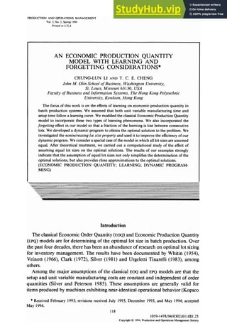
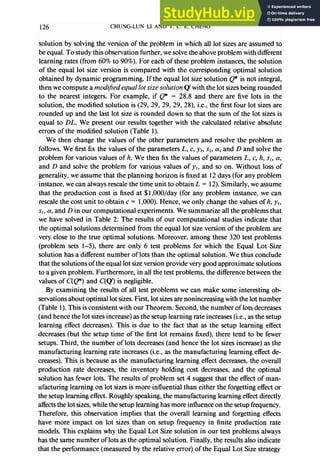
(A7) The inventory holding costper item per unit time is constant, i.e., indepen-
dent of the production cost
Assumptions A 1and A2 arethe basicassumptions usedin the classicalEOQ model
(Hadley and Whitin 1963; Silver and Peterson 1985). Assumption A3 ensuresthat
there is no shortage at the beginning of the planning horizon. Assumption A4 is
appropriate for situations where the operation performed has a large proportion of
human agency,suchasassembly.However, interruptions to the operation will cause
partial loss in learning, as stated in assumption A5. This is because relearning is
necessaryto revert to the productivity level attained before interruption occurred
(Keachie and Fontana 1966).Assumption A6 statesthat the costof one unit of time
of the facility is constant, that is,the costof spending one unit of time on a setup is
the same as the cost of spending one unit of time on manufacturing. Assumption
A7 is appropriate when aproduct’s storagecostis relatively high compared to labor
and material costsand the interest rate. This isbecausethe storagecostper item per
unit time is independent of the cost of producing the item.
From the learning curve equation (l), the variable manufacturing costof the ith
unit produced is
Cyj = cy,P.
Similarly, the costof the kth setup is
where b 5 0 is the learning index of the setup operation. Throughout our present
work, we assume- 1< a, b 5 0, since, for most practical situations, the values of a
and bare greater than - 1(Argote and Epple 1990).
From assumption A4, afraction (Yof the total learning islostbetween consecutive
production lots. Thus, the time required to produce the ith unit in the kth lot is
Yd( 1 - dzk + il”, (2)
where Zk = Q, + . . l + Q&r isthe number of units produced in the k - 1previous
lots (Z, = 0). Here we assumethat a fraction of the total learning is lost between
production lots.Alternatively, wemay usean assumption specifyingthe lossasrelative
to what hasbeenlearnt in the lust lot produced. However, suchan assumption would
lead to a more complex model to which the dynamic programming approach de-
scribed later cannot be applied.
Optimal Lot Sizes
Expression (2) implies that the total production time of the kth lot is
Qk (I-&k+Qk
tk = tk(&, zk) = 2 y,[( 1 - a)& + i]" = y] 2 i". (3)
i=l i’( f -a)&+ 1
Using the approximation CT=,i“ m ji x”&, we have
s
(I-a)Zk+C?k
tk = Y1 x%/x= --& {[(I - CY)z, + Q$+’ - [(l - (Y)&l(l+‘}. (4)
(I-@k
To calculate the inventory holding cost incurred in the kth lot, we first observe that
[from (4)] the time required to produce a quantity Q in the kth lot is given by

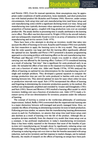
5. 122 CHUNG-LUN LI AND T. C. E. CHENG
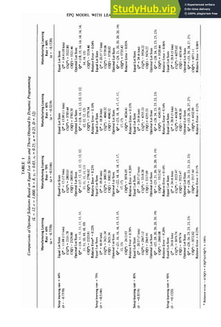
t(Q) = -& { [( 1 - a)& + Q]“” - [( 1 - CX)&]~+‘)
or, equivalently, the quantity produced in t units of time in the kth lot is given by
l
(a+1)t
I
I/(a+l)
MO
= y,
- + [( 1 - a)&~+’ - (1 - a)&
for 0 I t I tk. On the other hand, the quantity consumed during t units of time is
Dt. Therefore, the inventory level at time t in the kth production period is
iI(a + 1)t m+l)
- + [( 1 - (Y)z$+’
I(t)
= Yl I
-(I-a)&-&, if octet,
Q/c - Dt, if tk
< t5 Qk/o.
Thus, the holding cost of the kth lot is
s
C&ID
h I(t)& = h
0
[( 1 - c.u)z, + Qk]“+2 - ---$ [( 1 - a)&]a+2
-(I -C@&-T+Q @-t
’ k(D k)-;[($hij
= h --& [( 1 - a)& + Qk]a+2 - --& [( 1 - a)Z,$+2
e’
- [( 1 - dzk + Qk]fk + 20
I
. (5)
Hence, the total cost of the kth lot is
ck(Qk, z,) = CS,kh + ctk + h --& [(I - a)zk + Qkla+2
- -& [(1- &)&]a+2- e’k
[(1-a)Zk+ti?kh+~ ,
I
where tk is given in (4). Note that this total cost function includes the setup, production,
and inventory holding costs. It does not include any sunk cost (e.g., material cost or
overhead cost).
Note that ck(Qk, zk) only depends on k, Qk, and zk. Hence, we can use the following
dynamic program to solve for the optimal values of m and Qi, Q2, . . . , Qm.
(I) Define&(X) = the cost of an optimum production schedule for k lots consisting
of a total of X units such that the size of the last lot must be large enough so that
the kth cycle time less the production time in the kth cycle is at least s,(k + l)b.
(II) Recurrence relation:
fko =min c&!/c,
x - Q/c)
+h-I(X- Qk)
Qk= I,..., X - k + 1 and % - t&k, X - Qk) 2 sl(k + l)b
I
.

6. EPQ MODEL WITH LEARNING AND FORGETTING 123
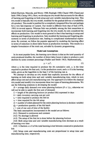
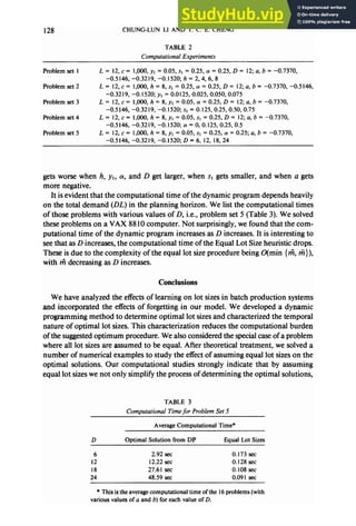
(III) Boundary conditions:
(IV) Optimal solution = min, cfh}, where
fl~=min{Cm(Q~,DL-Qm)+fm-l(DL-Qm)IQm= l,...,DL-m+ l}.
Let T be the total setup time and processing time of all the lots (except the setup
time of the first lot which is done before the planning horizon). Then
which implies
1 1
ll(b+l)
+1 .
Define
fi = min
L _ YdDL)a+l
a+
l )+ll’w”)],DL],
where 1x1denotes the largest integer no greater than x. Then the optimal solution in
(IV) is given by min {f,f;, . . . ,f k}. Since Qk, X I DL in the recurrence relation,
the computational complexity of this dynamic program is O((DL)2rti) I O((DL)3).
However, the nonincreasing lot size property stated in the theorem below can help
us improve the efficiency of the dynamic program.
THEOREM. The above dynamic program will generate an optimal solution with
nonincreasing lot sizes, that is, @ 2 Q$ 2 . . . 2 Q$$.
Proof: See Appendix.
Because of the above theorem, the recurrence relation in the dynamic program can
be modified to restrict the kth lot size to Qk = 1, . . . , LX/k]. Thus, Qk I DL/k, and
the computational complexity of the dynamic program reduces to O((DL) Cg:=, (DL/
k)) = O((DL)2 log Fz) I O((DL)2 log (DL)). Note that this result is based on the
assumption that the per unit inventory holding cost is independent of the per unit
production cost (assumption A7). Smunt and Morton (1985) studied a learning effect
model where the inventory holding cost of an item is proportional to its production
cost and their results appear to favor increasing lot sizes.
Equal Lot Sizes
We now consider a special case of the model where all lot sizes are equal, i.e., Q,
= Q2 = . . . = Q,,, = Q (Q E R+). This assumption will simplify the process of
determining the optimal lot sizes. Under this assumption, the total number of orders
will be
m = DL/Q.

7. 124 CHUNG-LUN LI AND T. C. E. CHENG
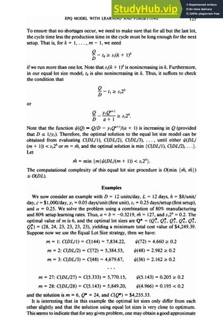
It follows that the total cost of operating the inventory system is given by
DUQ
C(Q) = c CkK?, (k - l>Q>
k=l
= D~[~~,~+d~+~{[(l -&- I)+ 1]“+2-[(1 -‘#-- 1)]“+2}
k=l
he’
- hQ[(l- a)(k- 1)+ l]tk+20
I
=Dy [cs,lp
+5 {[(I - a)(k - 1) + l]a+’ - [( 1 - a)(k - l)]““}
k=l
+ hyQ’+2
a+2 {[( 1 - (Y)(k - 1) + l]a+2 - [(I - Cx)(k- 1)3”‘2}
hy, e””
- a+l {[( 1 - a)(k - 1) + 11a+2- [( 1 - a)(k - 1)]“‘2
he’
-[(I -a)#- l)]““} +z
I
.
Note that
and
2 [(I -Cx)(k- l)]“=(l -cu)u c (k- 1)
k=l k=l
m (1 - q spL’Q-’
x”&=‘:4’” r$ - y,
and
DLIQ DUQ
kz, [(I - a)(k - 1) + 11” = (1 - cr)u c (k - 1 + l/(1 - a))
k=l
Thus,
+ cy,py1 - a)a+’
(a + l)(a + 2)
hy,pt2( 1 - CY)=+~ DL
- (a + l)(a + 2)(a + 3)
--l+l,(l-a)y+3-($-l)‘lf3]
Q
+ hy,@+2(1 - ~~y)a+’
(a + l)(a + 2)

8. EPQ MODEL WITH LEARNING AND FORGETTING 125
To ensure that no shortagesoccur, we needto make surethat for all but the last lot,
the cycletime lessthe production time in the cyclemust belong enough for the next
setup.Thatis,fork= l,..., m-1,weneed
ii? - tk 2 s,(k + 1)’
D
if we run more than one lot. Note that sl(l + l)b is nonincreasing in k. Furthermore,
in our equal lot sizemodel, tk is also nonincreasing in k. Thus, it suffices to check
the condition that
Q
- - tl 2 s,26
D
or
Note that the function $(Q) = Q/D - ~+@+‘/(a + 1) is increasing in Q (provided
that D 5 l/v,). Therefore, the optimal solution to the equal lot sizemodel can be
obtained from evaluating C(DL/l), C(DL/2), C(DL/3), . . . , until either $(DL/
(m + 1)) < ~~2~
or m = %, and the optimal solution ismin {C(DL/l), C(DL/2), . . .}.
Let
ti = min {ml$jDL/(m + 1)) < ~~2~).
The computational complexity of this equal lot sizeprocedure is O(min {fi, m})
5 o(DL).
Examples
We now consider an example with D = 12units/day, L = 12days,h = $8/unit/
day,c = $1,OOO/day,
yI = 0.05 days/unit (first unit), sI = 0.25 days/setup(first setup),
and r~= 0.25. We solve the problem using a combination of 80% manufacturing
and 80%setup learning rates.Thus, a = b = -0.32 19,% = 127,and ~~2~
= 0.2. The
optimal value of m is 6, and the optimal lot sizesare Q* = (Q:, Q:, Q:, Qf, QT,
Qz) = (28, 24, 23, 23, 23, 23), yielding a minimum total cost value of $4,249.39.
Supposenow we usethe Equal Lot Sizestrategy,then we have:
m = 1: C(DL/l) = C(144) = 7,834.22, t&72) = 4.660 r 0.2
m = 2: C(DL/2) = C(72) = $384.55, #(48) = 2.982 r 0.2
m = 3: C(DL/3) = C(48) = 4,679.67, +(36) = 2.162 2 0.2
ti = 27: C(DL/27) = C(5.333) = 5,770.15, ti(5.143) = 0.205 r 0.2
m = 28: C(DL/28) = C(5.143) = 5,849.20, ti(4.966) = 0.195 < 0.2
and the solution is m = 6, p = 24, and C(p) = $4,255.33.
It is interesting that in this example the optimal lot sizesonly differ from each
other slightly and that the solution using equal lot sizesis very closeto optimum.
This seemsto indicate that for anygiven problem, onemay obtain agood approximate

9. 126 CHUNG-LUN LI AND T. C. E. CHENG
solution by solving the version of the problem in which all lot sizes are assumed to
be equal. To study this observation further, we solve the above problem with different
learning rates (from 60% to 90%). For each of these problem instances, the solution
of the equal lot size version is compared with the corresponding optimal solution
obtained by dynamic programming. If the equal lot size solution @ is not integral,
then we compute a modljied equal lot sizesolution Q’ with the lot sizes being rounded
to the nearest integers. For example, if Q* = 28.8 and there are five lots in the
solution, the modified solution is (29, 29, 29, 29, 28), i.e., the first four lot sizes are
rounded up and the last lot size is rounded down so that the sum of the lot sizes is
equal to DL. We present our results together with the calculated relative absolute
errors of the modified solution (Table 1).
We then change the values of the other parameters and resolve the problem as
follows. We first fix the values of the parameters L, c, y,, sI, (Y,and D and solve the
problem for various values of h. We then fix the values of parameters L, c, h, sI, a,
and D and solve the problem for various values of yl, and so on. Without loss of
generality, we assume that the planning horizon is fixed at 12 days (for any problem
instance, we can always rescale the time unit to obtain L = 12). Similarly, we assume
that the production cost is fixed at $1 ,OOO/day (for any problem instance, we can
rescale the cost unit to obtain c = 1,000). Hence, we only change the values of h, yI,
sl, CY,
and D in our computational experiments. We summarize all the problems that
we have solved in Table 2. The results of our computational studies indicate that
the optimal solutions determined from the equal lot size version of the problem are
very close to the true optimal solutions. Moreover, among these 320 test problems
(problem sets l-5), there are only 6 test problems for which the Equal Lot Size
solution has a different number of lots than the optimal solution. We thus conclude
that the solutions of the equal lot size version provide very good approximate solutions
to a given problem. Furthermore, in all the test problems, the difference between the
values of C(Q*) and C(Q’) is negligible.
By examining the results of all test problems we can make some interesting ob-
servations about optimal lot sizes. First, lot sizes are nonincreasing with the lot number
(Table 1). This is consistent with our Theorem. Second, the number of lots decreases
(and hence the lot sizes increase) as the setup learning rate increases (i.e., as the setup
learning effect decreases). This is due to the fact that as the setup learning effect
decreases (but the setup time of the first lot remains fixed), there tend to be fewer
setups. Third, the number of lots decreases (and hence the lot sizes increase) as the
manufacturing learning rate increases (i.e., as the manufacturing learning effect de-
creases). This is because as the manufacturing learning effect decreases, the overall
production rate decreases, the inventory holding cost decreases, and the optimal
solution has fewer lots. The results of problem set 4 suggest that the effect of man-
ufacturing learning on lot sizes is more influential than either the forgetting effect or
the setup learning effect. Roughly speaking, the manufacturing learning effect directly
affects the lot sizes, while the setup learning has more influence on the setup frequency.
Therefore, this observation implies that the overall learning and forgetting effects
have more impact on lot sizes than on setup frequency in finite production rate
models. This explains why the Equal Lot Size solution in our test problems always
has the same number of lots as the optimal solution. Finally, the results also indicate
that the performance (measured by the relative error) of the Equal Lot Size strategy

10. TABLE 1
Comparisons of Optimal Solutions Based on Equal Lot Sizes and Those Obtained by Dynam
(L = 12, c = 1,000, h = 8, yI = 0.05, sI = 0.25, cx= 0.25, D = 12)
Manufacturing Learning
Rate = 60%
(a = -0.7370)
Manufacturing Learning
Rate = 70%
(a = -0.5 146)
Manufacturing
Rate = 80
(a = -0.3219
Setup learning
(b = -0.7370)
Setup learning
(6 = -0.5 146)
Setup learning
(b = -0.32 19)
Setup learning
(b = -0.1520)
rate = 60%
rate = 70%
rate = 80%
rate = 90%
Equal Lot Sizes
Q* = 11.08 ( 13 lots)
C(Q*) = 2331.78
C(Q’) = 2329.00
Optimal Lot Sizes
Q* = (16, 11, 11, 11, 11, 11, 11,
11, 11, 10, 10, 10, 10)
C(Q*) = 2323.81
Relative Error* = 0.22%
Equal Lot Sizes
Q* = 16 (9 lots)
C(Q*) = 2621.34
C(Q’) = 2621.34
Optimal Lot Sizes
Q* = (21, 16, 16, 16, 15, 15, 15,
15, 15)
C(Q*) = 2613.93
Relative Error = 0.28%
Equal Lot Sizes
Q’ = 20.57 (7 lots)
C(Q*) = 2867.12
C(Q’) = 2865.91
Optimal Lot Sizes
Q* = (25, 20, 20, 20, 20, 20, 19)
C(Q*) = 2860.08
Relative Error = 0.20%
Equal Lot Sizes
Q* = 24 (6 lots)
C(Q*) = 3079.74
C(Q’) = 3079.74
Optimal Lot Sizes
Q” = (28, 24, 23, 23, 23, 23)
C(Q*) = 3072.82
Relative Error = 0.23%
Equal Lot Sizes
Q* = 12 (12 lots)
C(Q*) = 2803.01
C(Q’) = 2803.01
Optimal Lot Sizes
Q’ = (17, 12, 12, 12, 12, 12, 12,
11, 11, 11, 11, 11)
C(Q*) = 2796.62
Relative Error = 0.23%
Equal Lot Sizes
Q* = 18 (8 lots)
C(Q*) = 3082.20
C(Q’) = 3082.20
Optimal Lot Sizes
Q” = (22, 18, 18, 18, 17, 17,
17, 17)
Equal Lot Sizes
Q* = 13.09 ( 11 lots
C(Q*) = 3785.44
C(Q’) = 3783.50
Optimal Lot Sizes
Q” = (18, 14, 13,
12, 12, 12, 12)
C(Q*) = 3779.54
Relative Error = 0.10%
Equal Lot Sizes
Q* = 18 (8 lots)
C(Q*) = 4040.32
C(Q’) = 4040.32
Optimal Lot Sizes
Q* = (23, 18, 18,
17, 17)
C(Q*) = 3076.05 C(Q*) = 4034.41
Relative Error = 0.20% Relative Error = 0.15%
Equal Lot Sizes Equal Lot Sizes
Q* = 20.57 (7 lots) Q* = 24 (6 lots)
C(Q*) = 3318.38 C(Q*) = 4255.33
C(Q’) = 3317.09 C(Q’) = 4255.33
Optimal Lot Sizes Optimal Lot Sizes
Q* = (25, 21, 20, 20, 20, 19, 19) Q* = (28, 24, 23,
C(Q*) = 3312.42 C(Q*) = 4249.39
Relative Error = 0.14% Relative Error = 0.14%
Equal Lot Sizes Equal Lot Sizes
Q* = 24 (6 lots) Q* = 28.8 (5 lots)
C(Q*) = 3523.47 C(Q*) = 4438.97
C(Q’) = 3523.47 C(Q’) = 4438.30
Optimal Lot Sizes Optimal Lot Sizes
Q* = (28, 24, 23, 23, 23, 23) Q* = (33, 29, 28, 2
C(Q*) = 35 17.40 C(Q*) = 4432.99
Relative Error = 0.17% Relative Error = 0.12%
* Relative error = (C(Q’) - C(Q*))/C(Q*) X 100%.

11. 128 CHUNG-LUN Ll AND T. C. E. CHENG
TABLE 2
Computational Experiments
Problem set 1 L = 12, c = 1,000, yI = 0.05, s1 = 0.25, (Y= 0.25, D = 12; a, b = -0.7370,
-0.5146, -0.3219, -0.1520; h = 2,4, 6, 8
Problem set 2 L = 12, c = 1,000, h = 8, s, = 0.25, (Y= 0.25, D = 12; a, b = -0.7370, -0.5146,
-0.3219, -0.1520; y, = 0.0125, 0.025,0.050,0.075
Problem set 3 L = 12, c = 1,000, h = 8, yI = 0.05, a = 0.25, D = 12; a, b = -0.7370,
-0.5146, -0.3219, -0.1520; s, = 0.125,0.25, 0.50,0.75
Problem set 4 L = 12, c = 1,000, h = 8, yl = 0.05, s, = 0.25, D = 12; a, b = -0.7370,
-0.5146, -0.3219, -0.1520; (Y= 0,0.125,0.25, 0.5
Problem set 5 L = 12, c = 1,000, h = 8, yl = 0.05, s, = 0.25, cr = 0.25; a, b = -0.7370,
-0.5146, -0.3219, -0.1520; D = 6, 12, 18, 24
getsworse when h, yI, (Y,and D get larger, when sI gets smaller, and when a gets
more negative.
It isevident that the computational time of the dynamic program depends heavily
on the total demand (DL) in the planning horizon. We list the computational times
of those problems with various values of D, i.e., problem set5 (Table 3). We solved
theseproblems on a VAX 88IOcomputer. Not surprisingly, we found that the com-
putational time of the dynamic program increasesasD increases.It isinteresting to
seethat asD increases,the computational time of the Equal Lot Sizeheuristic drops.
Theseisdue to the complexity of the equal lot sizeprocedure being O(min {$z,Cz}),
with A decreasing asD increases.
Conclusions
We have analyzedthe effectsof learning on lot sizesin batch production systems
and incorporated the effects of forgetting in our model. We developed a dynamic
programming method to determine optimal lot sizesand characterizedthe temporal
nature of optimal lot sizes.This characterization reducesthe computational burden
of the suggestedoptimum procedure. We alsoconsideredthe specialcaseof aproblem
where all lot sizesare assumedto be equal. After theoretical treatment, we solved a
number of numerical examplesto study the effect of assuming equal lot sizeson the
optimal solutions. Our computational studies strongly indicate that by assuming
equal lot sizeswe not only simplify the processof determining the optimal solutions,
TABLE 3
Computational Time for Problem Set 5
Average Computational Time*
D Optimal Solution from DP Equal Lot Sizes
6 2.92 set 0.173 set
12 12.22 set 0.128 set
18 27.61 set 0.108 set
24 48.59 set 0.091 set
* This is the average computational time ofthe 16problems (with
various values of a and b) for each value of D.

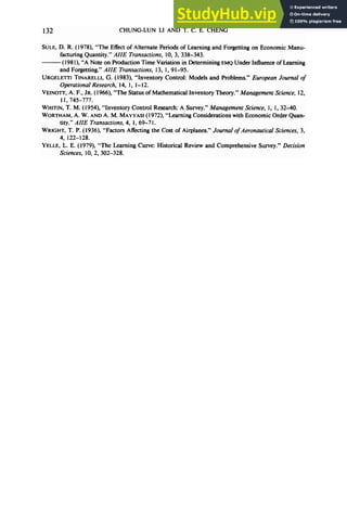
12. EPQ MODEL WITH LEARNING AND FORGETTING 129
but we can also provide close approximations to the optimal solutions. In other
words, although both manufacturing and setup learning effects may affect our decision
in selecting lot sizes, the “equal lot size rule” performs very well under these learning
and forgetting considerations. Furthermore, we show that the forgetting effect appears
to be less influential than the learning effect.’
’ We thank the referees for their helpful comments and suggestions. We are grateful to the associate
editor for providing the idea of the proof of the Theorem in this paper. We also thank Professor Maurice
Queyranne (Faculty of Commerce, University of British Columbia) for proving the Lemma in the Ap
pendix.
Appendix
To prove the Theorem, we first consider the following lemma.
LEMMA. Define
G(x, y, s, t) = {(x + t)2-y - (x + 1)2-y + (x + st + 1)2-y - (x + s + t)2-y + (x + s)*-~ - (x + ~t)*-~}/
(2 - y) + {(x + l)[(x + I)‘--y - x1-q + (x + s + f)[(X + s + t)‘-y - (x + s)‘-q
- (x + l)[(X + tp - x-j -.(x + sr + l)[(x + St + 1)1-y - (x -t st)‘-q}/( 1 - y).
ThenG(x,y,s,t)rO,foranyx,yzO(yP 1,2)ands,tE(O, 1).
Proof of Lemma. Define g(t) = G(x, y, s, t). It is easy to check that g(O) = g( 1) = 0, and that the
second derivative of g is
s”(l) = (x + s + tp - (x + t)-’ + sz[(x + sty - (x + St + 1)-y - y(x + sty-‘]
5 $[(x + sty - (x + Sl + 1)--Y- v(x + sty-‘].
Let y(u) = 0. By the Mean Value Theorem, there exists [ E (x + sf,x + st + I) such that
y(x + St + 1) - y(x + St) = r’(S)
or
(x+st+ I)‘-(x+st)-y= -yp-‘.
Thus,
g”(t) s s’y[p-’ - (x + st)p--‘1 s 0.
Therefore, g(f) is concave in (0, l), and g(t) t 0 for all t E (0, 1). Q.E.D.
ProofofTheorem. Suppose, to the contrary, that in the optimal solution there are two successive lots
k and k + 1 such that Q: < Qz+i. Then we consider a new solution (Q:, . . . , Qz-‘, Qz++,, Q:, Qz+;2,
. . . , Qz) after switching the sizes of these two lots. Note that a switch of two lots will not affect the total
setup cost, and that if the original schedule (Q:, . . . , Qz) does not incur any shortages, then neither
does the new schedule. Moreover, a switch of two successive lots will not affect the manufacturing costs
and the inventory holding costsof the other lots. We shall show that after this switch, (i) the manufacturing
cost of lots k and k + 1 will not go up and (ii) the holding cost of lots k and k + 1will not go up.
(i) In the original solution (Q:, . . . , Q:), the processing time of lots k and k + 1is
tk+fk+l = --& { [( 1 - cr)Z: + Q:1”+’ - [( 1 - a)Z:l”+’
+ [(I - 4(Z: + Q:, + Q;+$‘+’ - [(I - a)(Zks + Qk’,Y+‘},
where Z: = Q:, . . . , QfTl. Let I; and f(k+’ be the new processing time of lots k and k + 1, respectively.
Then
t; + ti+’ a --& {[(l - o)Z: + Q;+J+’ - [(I - a)Z:]II+’
+ [Cl - cW: + Q;+I) + Q; O+’
1 - [(I - a)(Z; + Q;+,,la+‘}.

13. 130 CHUNG-LUN LI AND T. C. E. CHENG
Letu=Q:>O,u=Qz+‘-Q:>O,andA=(l-a)(Z:+Qz)rO.Then
and
tk+tk+l = --J& {[A + auy+ - [,4 - (1 - c&y+’ + [‘4 + u + ul”+’ - A’+‘}
t; + t;+, = --& {[A + CYU
+ uy+ - [‘4 - (1 - a)#+’ + [A + u + (1 - cu)u]“+’ - [A + (1 - cy)uy+‘}.
Define
flx)=[‘4+xu]“+‘-[A+xu+u]“+‘+[‘4+(1-x)u]a+’
- [A + 24+ (1 - x)ul”+’ + [A + 24+ u]“+’ - A”+‘,
for 0 s x 5 1. It is easy to check that F(0) = F( 1) = 0, and that the second derivative of this function is
F”(x) = a(a + l)uz
1
1 1
-
(‘4 + xup (PI + xu + u)‘-O1
lN2 I
1 1
+ da + (A + (1 - x)u)‘-a - (A + u + (1 - x)u)‘-’ 1
S O
for any a 5 0. Thus, F(x) is concave in (0, l), and F(x) 2 0 for all x E [0, 11.Hence, we have
(tk + tk+l) - (ti, + ti+l) = --$ F(a) 2 0,
or
ti + t;+l 5 tk+ tk+‘.
(ii) Let hk and hk+’ be the holding costs of lots k and k + 1, respectively, in the original solution. Let
/& and wk+’ be the holding costs of lots k and k + 1, respectively, in the new solution. Then, from (5),
hk + hk+’ = h
I
--& [(l - LY)Z: + Q;]Il+’ - -& [(l - a)Z:1”+*
Q:’
- [(I - a)z: + Q:]tk + - +
2D --& I(1 - 4(Z: + Q:, + Q;+d”+’
- --$ [(I - a)(Z: + Q:)1”+’ - [(I - d(z: + Q:, + Q:+&+l + g]
and
h;, + kk+’ = h
I
-& [(l - ~y)Zt + Q;+‘]“+* - --$ [(l - (Y)Z:~“+*
**
&+I
- [(I - a)Z: + Q:+,]ti + - +
20
--& [(I - aXZ: + Q:+:;,,+ Q:Y+’
- --& [(I - aWk* + Q:+,,l”+* - [(I - 4tZ: + Q;+I) + Q:lti+, + g
I
.
Hence,
(hk + hk+l) - (hk + hk+l)
= hyl
I
-& [( 1 - a)Z: + Q:y+* - -& [(I - a)Z: + Q~+J’+’
+ --& [(I - aW: + Q:, + Qk,Y+’ - --& [(l - 4(Z: + Q:+I, + Q:l=+*
+ & N1- dot: + Q;+N+’ - -& Kl - 4(Z: + ,:I,,+*
- --& [(I - a)Z: + Q:J{[(l - a)Z: + Q:1.+’ - [(l - cu)Z:]‘+‘)

14. EPQ MODEL WITH LEARNING AND FORGETTING 131
--&I(1 - 4(Zk*+Q:, +Q:+J{Nl - 4V: + Q:, + Q:+t;,Y+'
- [(I - 4(Zk*+Qk*,,"")
+--&(I - 4.Z: + Q:+J{Nl - cWk*
+Q~+,la+'
- [Cl- a)Zk*ln+')
+& [(I - 4(Zk*+ Q;+d+ Q:lW - 4@: + Qkd + Qk*l'+'- [(I - 4(zk*+Q;+X+',]
=h~,(Q;+d=+~*
G((1- aP:/Q:+,, -a, I - a,Q:/Q:+d2 0. (by Lemma)
Therefore,
h; + h;+, I hk + h&l. Q.E.D.
References
ALDER, G. L. (1973) The Eflects of Learning on Optimal Single and Multiple Lot Size Determination,
Unpublished Ph.D. dissertation, New York University.
- AND R. NANDA (1974a), “The Effects of Learning on Optimal Lot Size Determination-Single
Product Case,” AIIE Transactions, 6, 1, 14-20.
-AND R. NANDA (1974b), “The Effectsof Learning on Optimal Lot Size Determination-Multiple
Product Case.” AIIE Transactions, 6, 1, 21-27.
ARGOTE, L. AND D. EPPLE (1990), “Learning Curves in Manufacturing.” Science, 247, 920-924.
AXSATER, S. AND S. E. ELMAGHRABY (198 I), “A Note on EMQ under Learning and Forgetting.” AIIE
Transactions, 13, 1, 86-90.
BUFFA, E. S. (1984), Meeting the Competitive Challenge, Irwin, Homewood.
CARLSON, J. G. H. (1975), “Learning, Lost Time and Economic Production (the Effects of Learning on
Production Lots).” Production and Inventory Management, 16, 4th Quarter, 20-33.
CHAND, S. (1989), “Lot Sizes and Setup Frequency with Learning in Setups and Process Quality.”
European Journal of Operational Research, 42, 2, 190-202.
AND S. SETHI (1990), “A Dynamic Lot Sizing Model with Learning in Setups.” Operations
Research, 38,4, 644-655.
CHENG, T. C. E. (1991), “An EOQ Model with Learning Effect on Setups.” Production and Inventory
Management, 32, 1st Quarter, 83-84.
- AND S. PODOLSKY (1993), Just-in-Time Manufacturing An Introduction, Chapman and Hall,
London.
CLARK, A. J. (1972), “An Informal Survey of Multi-Echelon Inventory Theory.” Naval Research Logistics
Quarterly, 19, 4, 62 I-650.
HADLEY, G. AND T. M. WHITIN (1963), Analysis oflnventory Systems, Prentice-Hall, New Jersey.
KARWAN, K. R., J. B. MAZZOLA, AND R. C. MOREY (1988) “Production Lot Sizing under Setup and
Worker Learning.” Naval Research Logistics, 35, 2, 159-175.
KEACHIE, E. C. AND R. J. FONTANA (1966), “Effects of Learning on Optimal Lot Size.” Management
Science, 13, 2, Bl02-B108.
KOPSCO, D. P. AND W. C. NEMITZ (1983), “Learning Curves and Lot Sizing for Independent and
Dependent Demand.” Journal of Operations Management, 4, 1, 73-83.
NADLER, G. AND W. D. SMITH (1963), “Manufacturing Progress Functions for Types of Processes.”
International Journal of Production Research, 2, 2, 115- 135.
REPLOCLE, S. H. (1988), “The Strategic Use of Smaller Lot Sizes Through a New EOQ Model.” Production
and Inventory Management, 29, 3rd Quarter, 4 l-44.
SCHONBERGER, R. (1982), Japanese Manufacturing Techniques: Nine Hidden Lessons in Simplicity,
Free Press, New York.
SILVER, E. A. (198 1), “Operations Research in Inventory Management: A Review and Critique.” Op-
erations Research, 29, 4, 628-645.
- AND R. PETERSON(1985), Decision Systemsfor Inventory Management and Production Planning,
2nd ed., John Wiley & Sons, New York.
SMUNT, T. L. AND T. E. MORTON (1985), “The Effectof Learning on Optimal Lot Sizes.” ZZETransactions,
17, 1, 33-37.
SPRADLIN, B. C. AND D. A. PIERCE (I 967), “Production Scheduling under a Learning Effect by Dynamic
Programming.” Journal of Industrial Engineering, 18, 3, 219-222.

15. 132 CHUNG-LUN LI AND T. C. E. CHENG
SULE, D. R. (1978), “The Effect of Alternate Periods of Learning and Forgetting on Economic Manu-
facturing Quantity.” AIIE Transactions,
10, 3, 338-343.
- (198 l), “A Note on Production Time Variation in Determining EMQ Under Influence of Learning
and Forgetting.” AIIE Transactions,
13, 1,9 l-95.
URGELEI-TI TINARELLI, G. (1983), “Inventory Control: Models and Problems.” European
Journalof
Operational
Research,
14,1, I- 12.
VEINOTT, A. F., JR. (1966), “The Status of Mathematical Inventory Theory.” Management
Science,
12,
11,745-777.
WHITIN, T. M. (1954), “Inventory Control Research: A Survey.” Management
Science,
1, 1, 32-40.
WORTHAM, A. W. AND A. M. MAYYASI (1972), “Learning Considerations with Economic Order Quan-
tity.” AIIE Transactions,
4, I, 69-71.
WRIGHT, T. P. (1936), “Factors Affecting the Cost of Airplanes.” JournalofAeronautical
Sciences,
3,
4, 122-128.
YELLE, L. E. (1979), “The Learning Curve: Historical Review and Comprehensive Survey.” Decision
Sciences,
10, 2, 302-328.