Adaptive Functional-Based Neuro-Fuzzy-PID Incremental Controller Structure

Indonesian Journal of Electrical Engineering and Informatics (IJEEI)
Vol. 2, No. 1, March 2014, pp. 24~47
ISSN: 2089-3272  24
Received January 16, 2014; Revised February 12, 2014; Accepted February 20, 2014
Adaptive Functional-Based Neuro-Fuzzy-PID
Incremental Controller Structure
AA Fahmya
, AM Abdel Ghanyb
Systems Engineering Department, Cardiff School of Engineering, Cardiff University
Cardiff CF24 3AA, U.K.
Electrical Power and Machines Department, Faculty of Engineering, Helwan University
Cairo, Egypt.
Abstract
This paper presents an adaptive functional-based Neuro-fuzzy-PID incremental (NFPID)
controller structure that can be tuned either offline or online according to required controller performance.
First, differential membership functions are used to represent the fuzzy membership functions of the input-
output space of the three term controller. Second, controller rules are generated based on the discrete
proportional, derivative, and integral function for the fuzzy space. Finally, a fully differentiable fuzzy neural
network is constructed to represent the developed controller for either offline or online controller parameter
adaptation. Two different adaptation methods are used for controller tuning, offline method based on
controller transient performance cost function optimization using Bees Algorithm, and online method based
on tracking error minimization using back-propagation with momentum algorithm. The proposed control
system was tested to show the validity of the controller structure over a fixed PID controller gains to control
SCARA type robot arm.
Keywords: Optimization techniques, adaptive control, Fuzzy systems, Neuro-Fuzzy-PID PID-controllers,
Neuro-fuzzy systems
1. Introduction
1.1. Background
Three term PID controller is one of the simplest and oldest control method utilized in
industry due to its simple structure and implementation that achieved good performance for
plenty of applications. Traditional PID controllers have been widely used for industrial processes
due to their simplicity and effectiveness for systems that can be modeled by mathematical
equations. Despite its simplicity, it is a linear controller and generally difficult to tune its
parameters to the desired performance all times, especially with nonlinear and complex systems
[Petrov et. al., 2002]. As a consequence of the rapid development in Fuzzy Logic Systems
(FLS) and Neural Networks (NN) techniques in the 1980s, great progress in Fuzzy PID
controller and fuzzy-Neural Networks (FNN) design and implementation techniques was made
[Sheroz et. al., 2008]. Fuzzy-PID controllers provide non-linear structure that, despite more
complex than simple linear PID controller, can achieve controller non-linearity needed to
achieve the desired control response in complex systems [Karasakal et. al., 2005]. Fuzzy logic
control (FLC) has found many successful industrial applications and demonstrated significant
performance improvements, as the controller structure gives flexibility to achieve either linear or
non-linear controller response [Baogang et al., 2001]. Most FLC can be classified into two types,
the gain-scheduling FPID type and the direct-action FPID type. In the gain-scheduling FPID
type, fuzzy inference is employed to compute the individual conventional PID gains [Huang and
Yasunobo, 2000]. The majority of FPID applications belong to the direct-action FPID type where
the direct-action FPID is placed within the feedback control loop to compute the control actions
through fuzzy inference [Ying, 1993]. Several direct-action FPID structures were reported using
one, two or three inputs (error, rate of change of error and integral of error) [Ying et al., 1990]. In
all of these direct-action FPID controllers, the derivative and integral functions are performed
quantitatively outside the FLC. They do not employ a FLS as a function approximation to
perform a fuzzy integral or fuzzy derivative function [Mann et. al., 1999]. In these controllers, the
FLS performs only the non-linear amplifications associated with the three PID control actions.
Therefore these controllers are actually Input-based FPID controllers (I-FPID) rather than

 ISSN: 2089-3272
IJEEI Vol. 2, No. 1, March 2014 : 24 – 47
25
Function-based FPID controllers (F-FPID) [Tang et. al., 2001]. In this paper, the controller
functionally performs fuzzy derivative and fuzzy integral functions, so that no calculations are
required outside the FLC. The proposed controller employs only two inputs (present and
previous errors), so that the design procedure is simpler. Additionally, most fuzzy logic based
PID controllers in literature adapt the triangular membership function shape for simplicity of
implementation, despite it’s linear nature. In this paper, other types of membership functions,
such as Gaussian, and sigmoid membership functions are utilized in the design of the controller
to allow tuning for the controller membership functions as well as online adaptation of the
controller based on the Back-propagation with momentum (BP) learning algorithm.
Since the early 1990s, FNN have attracted a great deal of interest because such
systems are more flexible and transparent than either NN or FLS alone. Different types of FNN
have been presented in the literature [Shing and Jang, 1993]. For tracking control where the
reference and dynamics is always changing, the inverse dynamic control is the best to be
utilized, despite very difficult to be implemented mathematically. Consequently, researcher
tends to use neural network and neuro-fuzzy systems to avoid complex mathematical
formulation [Sinthipsomboon et. al., 2011]. In [Anh and Pham, 2010] a gain-scheduling neural
PID controller is utilized with 2-axis robotic structure for varying the parameters of the neural
PID controller to include information from the robot dynamics. The FNN types can be identified
based on the structure of the FNN, the fuzzy model employed and the learning algorithm
adopted [Ahn and Anh, 2009]. On the other hand, the most commonly used and successful
approach is the feed-forward and recurrent structure model, while using the BP as the learning
algorithm [Yuan et. al., 1992, Nauck and Kruse 1993]. On the other hand, according to the fuzzy
model adopted, there are two types of fuzzy models that can be integrated with a neural
network to form a FNN [Anh, 2010]. These two models are the TS-model [Takagi and Sugeno,
1985] and the Mamdani-model [Lee, 1990a and 1990b]. However, Mamdani-model based FNN
represent all linguistic fuzzy representation compared with TS-model-based FFNN. In this
paper, Mamdani-model is utilized to construct a full-differential Neuro-Fuzzy PID controller that
can be adapted both off-line or on-line [Shing and Jang 1993].
1.2. Problem Statement
The best description of the problem statement of this research topic is how to construct
a functional based PID control that is performing the proportional, differential, and integral
operations on the fuzzy membership functions directly and affected only by the error value,
while constructing this controller in a computational format that can be easily adapted either off-
line or online using any available adaptation algorithm [Fahmy and Abdel Ghany 2013].
1.3. Objectives
Looking into the previous problem statement, the objectives of the research can be
summarized as:
1.3.1. Generate new definition for fuzzy proportional, differential, and integral functions.
1.3.2. Implement the controller calculation process into a full-differential Mamdani-model
neural network.
1.3.3. Define the neural network and its activation functions in a differentiable format.
1.3.4. Demonstrate the off-line and online adaptation capabilities of the suggested PID
controller.
The remainder of the paper aims to show the design processed and suggested
functions to meet the above objectives. The remainder of the paper is organized as follows.
Section (2) outlines the differential functional-based fuzzy PID controller. Section (3) presents
the overall structure of the proposed adaptive neuro-fuzzy PID controller. Section (4) describes
the off-line and on-line neuro-fuzzy PID controller tuning methods. Section (5) compares the
results of applying the proposed control system with those obtained with a conventional-PID for
a robotic-arm joint movement control. Section (6) represents a detailed discussion of the work
presented, while section (7) concludes the paper.
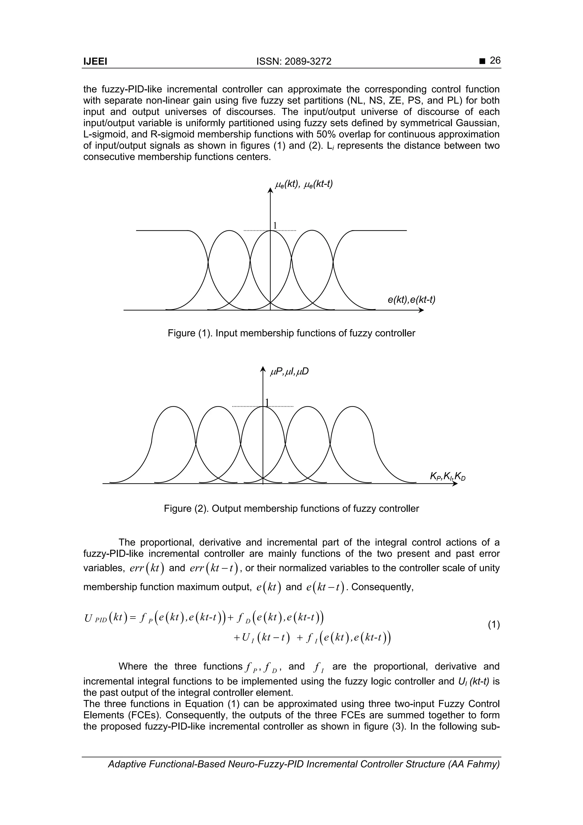
2. Differential Functional-Based Fuzzy PID controller
The suggested fuzzy-PID-like incremental controller employs two inputs (present and
previous errors) that are more convenient for digital controller implementation. Each element of

IJEEI ISSN: 2089-3272 
Adaptive Functional-Based Neuro-Fuzzy-PID Incremental Controller Structure (AA Fahmy)
26
the fuzzy-PID-like incremental controller can approximate the corresponding control function
with separate non-linear gain using five fuzzy set partitions (NL, NS, ZE, PS, and PL) for both
input and output universes of discourses. The input/output universe of discourse of each
input/output variable is uniformly partitioned using fuzzy sets defined by symmetrical Gaussian,
L-sigmoid, and R-sigmoid membership functions with 50% overlap for continuous approximation
of input/output signals as shown in figures (1) and (2). Li represents the distance between two
consecutive membership functions centers.
Figure (1). Input membership functions of fuzzy controller
Figure (2). Output membership functions of fuzzy controller
The proportional, derivative and incremental part of the integral control actions of a
fuzzy-PID-like incremental controller are mainly functions of the two present and past error
variables,  err kt and  err kt t , or their normalized variables to the controller scale of unity
membership function maximum output,  e kt and  e kt t . Consequently,
           
      
PID P D
I I
kt e kt ,e kt-t e kt ,e kt-tf fU
U kt t e kt ,e kt-tf
 
  
(1)
Where the three functions Pf , Df , and If are the proportional, derivative and
incremental integral functions to be implemented using the fuzzy logic controller and UI (kt-t) is
the past output of the integral controller element.
The three functions in Equation (1) can be approximated using three two-input Fuzzy Control
Elements (FCEs). Consequently, the outputs of the three FCEs are summed together to form
the proposed fuzzy-PID-like incremental controller as shown in figure (3). In the following sub-
1
P,I,D
KP,KI,KD
1
e(kt), e(kt-t)
e(kt),e(kt-t)

 ISSN: 2089-3272
27
sections, the design process of the operation rules for the three functions in Eq. (1) in the form
of three fuzzy control elements will be explained.
Figure (3). Structure of the fuzzy PID feedback controller
Each output function of the fuzzy PID-like incremental controller is of a different nature
(proportional, derivative, or integral). Therefore the partition of the output universe of discourse
is selected to be of the same membership function shape and degree of overlapping but with
different scaling factors to allow for different tuning of each control element.
2.1. Fuzzy Proportional Control Element
The fuzzy rules of the operation of the FPCE according to the suggested partitions are
generated heuristically based on the intuitive concept that the proportional control action at any
time step is directly proportionally to an error 1e at the same time step regardless of the value of
the error at the previous time step 2e . Therefore if the error variable 1e is expressed
linguistically as zero, negative small, or negative large, the proportional control action can be
expressed linguistically as zero, negative small, or negative large respectively, regardless of the
linguistic value of the error variable 2e . Consequently, the Fuzzy Associative Memory (FAM)
rules according to this concept of the FPCE can be written as shown in table (1).
Table (1). Proportional element FAM bank
2e
1e
NL NS ZE PS PL
NL NL NL NL NL NL
NS NS NS NS NS NS
ZE ZE ZE ZE ZE ZE
PS PS PS PS PS PS
PL PL PL PL PL PL
where [NL, NS, ZE, PS, PL] are the term sets of the normalized input variables 1e and
2e and the normalized output variable  P ktU . To infer the fuzzy output of the FPCE,
Mamdani’s min/max method using the bounded sum triangular co-norm is employed. In [Yuan
et al., 1992], the fmin and fmax functions were introduced to approximate the logic min and logic
max functions analytically. These two functions were formulated as follows:
e1=e(kt)
e2=e(kt-t)
+
UD
+
UP
UI
+
UPID
Proportional
FCE
Derivative
FCE
Integral
FCE
Z-1
KU

IJEEI ISSN: 2089-3272 
28
     
2 2
, 0.5 ( ) 0.01 0.01      
  
e1 2 e1 2 1 2e e e efmin h h h h h h (2)
     
2 2
, 0.5 ( ) 0.01 0.01
 
       
1 2 1 2 1 2p p p p p pfmax h h h h h h (3)
Where  1 2e eh and h are defined as the fuzzy membership function values of the input
error variables ( 1e and 2e ), while  p1 p2h and h are defined as the fuzzy membership function
values of the same output membership function resulting from any two different rules at any
time step. The centre average defuzzification method (Height method) [Ying et. al., 1990; Ying,
1993] is employed to calculate the crisp output of the FPCE. Consequently, based on the
defined membership functions, only four rules are triggered at a time. Therefore, the inference
system produces four non-zero fuzzy outputs for the two crisp error inputs. The fuzzy output of a
rule (output fuzzy sets after inference) is a fuzzy set with a flat-top Gaussian shape membership
function whose height (h) equals the membership degree produced by the min operator of Eq.
(2). Based on the input errors condition, employed inference method, and defuzzification
method, the output of the FPCE is calculated for any input condition using the centre average
defuzzification method, assuming different membership output function for each rule inference,
as follows:
(4)
i
i
output
1
1
4
Rulei=
4
Rulei=
h value of the input Mf with min h output Mf centre
h value of the input Mf with min h
FPCE 
 
  
 
  


Using Eq. (2) and Eq. (3), the analytical solution of the proportional function of the
FPCE  1 2,Pf e e in Eq. (1) can be expressed as follows:
   
   
1 2 1 2
1
1 2 1 2
1
4 2 2
4 2 2
2
0 01 0 01
0 01 0 01
(5)
i i i i i
i i i i
i
i
output
Rule
Rule
R R R R R
i
R R R R
i
*
CP ( (e ) (e )) (e ) (e ) . .
( (e ) (e )) (e ) (e ) . .
FPCE
   
   



  
  
  
  
 
 
 
 
    
    


where CPRi is the FPCE output membership function centre value for rule i, μRi(e1) is the
membership degree of the present error to the rule i, and μRi(e2) is the membership degree of
the past error to the rule i.
2.2. Fuzzy Derivative Control Element
In the case of the Fuzzy Derivative Control Element FDCE, the distance between the
centres of any two adjacent output membership functions is now LD. The fuzzy rules for the
operation of the FDCE according to the suggested partitions are generated heuristically as well
based on the intuitive concept that the derivative control action at any time step is directly
proportionally to rate of change of the error (difference between two successive time steps). For
example, if the error variables 1e and 2e are both expressed linguistically as positive, the
derivative control action can be expressed linguistically as zero. Consequently, the Fuzzy
Associative Memory (FAM) rules according to this concept of the FDCE can be written as
shown in table (2). Where [NL, NS, ZE, PS, PL] are the term sets of the normalized input
variables 1e and 2e and the normalized output variable  D ktU . Consequently, based on the
defined membership functions, only four rules are triggered at a time. The fuzzy output of a rule
(output fuzzy sets after inference) is a fuzzy set with a with a flat-top Gaussian shape

 ISSN: 2089-3272
29
membership function whose height (h) equals the membership degree produced by the min
operator of Eq. (2) during the fuzzy inference.
Table (2). Derivative element FAM bank
2e
1e
NL NS ZE PS PL
NL ZE NS NL NL NL
NS PS ZE NS NL NL
ZE PL PS ZE NS NL
PS PL PL PS ZE NS
PL PL PL PL PS ZE
Based on the input errors condition, employed inference method, and defuzzification
method used in the last section, the analytical solution of the FDCE function  1 2,Df e e in Eq.
(1) can be written as follows:
   
   
1 2 1 2
1
1 2 1 2
1
4 2 2
4 2 2
2
0 01 0 01
0 01 0 01
(6)
i i i i i
i i i i
output
i
i
R R R R R
i
Rule
R R R R
i
Rule
*
CD ( (e ) (e )) (e ) (e ) . .
( (e ) (e )) (e ) (e ) . .
FDCE
   
   



  
  
  
  
 
 
 
 
    
    


Where CDRi is the FDCE output membership function centre value for rule i, μRi(e1) is the
membership degree of the present error for the rule i, and μRi(e2) is the membership degree of
the past error for the rule.
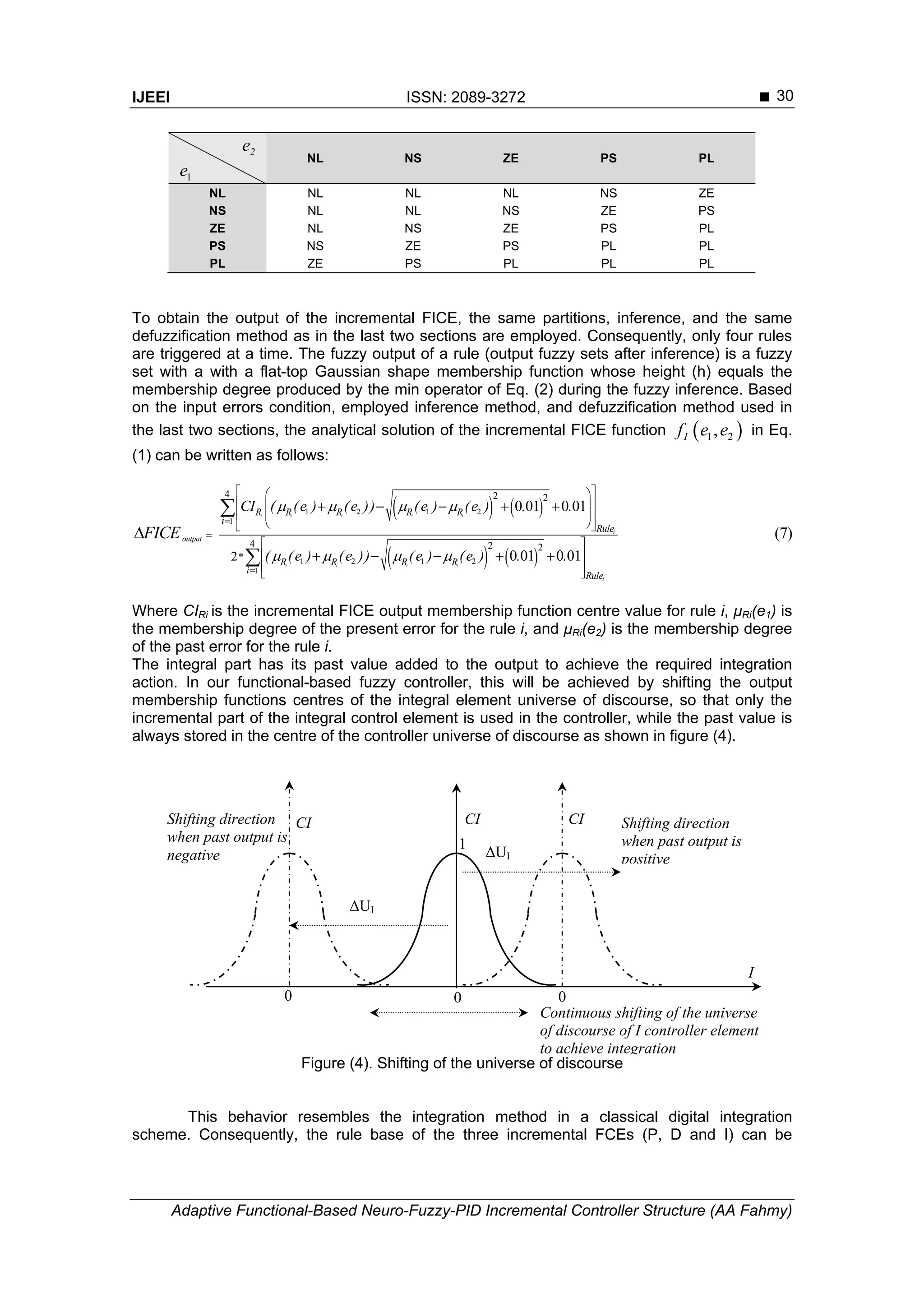
2.3. Fuzzy Incremental Integral Control Element
The conventional integral control action is composed of two parts. The first part is the
integration initial condition or the controller's output history  I kt-tU and the second part is the
controller's incremental output  1 2I I ktf (e ,e ) U  . Therefore, the output of the integral
element is composed of the same two parts. To implement the Fuzzy Integral Control Element
(FICE), the same numbers of input/output partitions as in the previous two sections are
employed. However, in this case, the distance between the centres of any two adjacent output
membership functions is LI. To implement the integration initial condition and the incremental
part into one fuzzy controller element, the centres of the output universe membership functions
are shifted after the kth
time step to a distance
1
0
( ) ( )
k
I I
m
mU kt t U t


   . The incremental part
of the integral control element is of interest now. The fuzzy rules of the operation of the
incremental FICE are generated heuristically based on the intuitive concept that the incremental
part of the integral control action at a time step is directly proportional to the sum of the error
variables at two successive time steps. For example, if the error variables 1e and 2e are
expressed linguistically as positive and negative, the incremental part of the integral control
action can be expressed linguistically as zero. Consequently, the Fuzzy Associative Memory
(FAM) rules according to this concept of the incremental FICE can be written as shown in table
(3). Where [NL, NS, ZE, PS, PL] are the term sets of the normalized input variables 1e and 2e
and the normalized output variable  I KTU .
Table (3). Integral incremental element FAM bank

IJEEI ISSN: 2089-3272 
30
2e
1e
NL NS ZE PS PL
NL NL NL NL NS ZE
NS NL NL NS ZE PS
ZE NL NS ZE PS PL
PS NS ZE PS PL PL
PL ZE PS PL PL PL
To obtain the output of the incremental FICE, the same partitions, inference, and the same
defuzzification method as in the last two sections are employed. Consequently, only four rules
are triggered at a time. The fuzzy output of a rule (output fuzzy sets after inference) is a fuzzy
set with a with a flat-top Gaussian shape membership function whose height (h) equals the
membership degree produced by the min operator of Eq. (2) during the fuzzy inference. Based
on the input errors condition, employed inference method, and defuzzification method used in
the last two sections, the analytical solution of the incremental FICE function  1 2,If e e in Eq.
(1) can be written as follows:
   
   
1 2 1 2
1
1 2 1 2
1
4 2 2
4 2 2
2
0 01 0 01
0 01 0 01
(7)
i i i i i
i i i i
i
i
output
R R R R R
i
Rule
R R R R
i
Rule
*
CI ( (e ) (e )) (e ) (e ) . .
( (e ) (e )) (e ) (e ) . .
FICE
   
   



  
  
  
  
 
 
 
 
    
    



Where CIRi is the incremental FICE output membership function centre value for rule i, μRi(e1) is
the membership degree of the present error for the rule i, and μRi(e2) is the membership degree
of the past error for the rule i.
The integral part has its past value added to the output to achieve the required integration
action. In our functional-based fuzzy controller, this will be achieved by shifting the output
membership functions centres of the integral element universe of discourse, so that only the
incremental part of the integral control element is used in the controller, while the past value is
always stored in the centre of the controller universe of discourse as shown in figure (4).
Figure (4). Shifting of the universe of discourse
This behavior resembles the integration method in a classical digital integration
scheme. Consequently, the rule base of the three incremental FCEs (P, D and I) can be
1
CI
I
0 00
CICI Shifting direction
when past output is
positive
Shifting direction
when past output is
negative
ΔUI
ΔUI
Continuous shifting of the universe
of discourse of I controller element
to achieve integration

 ISSN: 2089-3272
31
combined together to form one rule base for the total functional-based fuzzy-PID controller as
follows:
     
   
1 2 1 2
1
1 2 1 2
1
4 2 2
4 2 2
2
0 01 0 01
(8)
0 01 0 01
i i i i i i
i i i i
Ri R Rp d i
i
i
R R R Ru
i
Rule
R R R R
i
Rule
* CI CD CI
PID
*
( (e ) (e )) (e ) (e ) . .
( (e ) (e )) (e ) (e ) . .
k k k
U
k    
   


  
     
   

 
 
 
 
    
    


Where kp, kd, and ki are the scaling factors, while ku is an overall gain for the PID controller.
Table (4) represents the combined functional-based fuzzy-PID controller rules.
Table (4). Functional-Based fuzzy PID controller combined FAM bank
e1 e2 P-element D-element I-element
NL NL NL ZE NL
NS NL NS PS NL
ZE NL ZE PL NL
PS NL PS PL NS
PL NL PL PL ZE
NL NS NL NS NL
NS NS NS ZE NL
ZE NS ZE PS NS
PS NS PS PL ZE
PL NS PL PL PS
NL ZE NL NL NL
NS ZE NS NS NS
ZE ZE ZE ZE ZE
PS ZE PS PS PS
PL ZE PL PL PL
NL PS NL NL NS
NS PS NS NL ZE
ZE PS ZE NS PS
PS PS PS ZE PL
PL PS PL PS PL
NL PL NL NL ZE
NS PL NS NL PS
ZE PL ZE NL PL
PS PL PS NS PL
PL PL PL ZE PL
Finally, the total fuzzy-controller output can be represented in the form:
  ( )1 1 2 1 2PID U P NP D ND I NI
= + - + +e e e e eU k k k k k k k   (9)
Where kNP , kND , and kNI are the equivalent non-linear fuzzy gains.
3. Adaptive Neuro-Fuzzy PID Controller Structure
One of the main problems with conventional neuro-fuzzy controllers reported in
literature is the difficulty of applying sensitivity analysis or online-tuning methods due to the no-
differential shape of the triangular membership functions as well as the logic minimum and logic
maximum functions [Yuan et. al., 1992]. This in turn adds complexity to the speed and method
of on-line adaptation used. In the proposed controller, membership functions are replaced by
differentiable ones, as well as the logic minimum and logic maximum functions are replaced by
the softmin and softmax functions. The proposed structure of the fuzzy PID controller achieves
more flexibility for both online and offline tuning.

IJEEI ISSN: 2089-3272 
32
3.1. Softmin and Softmax Functions
The proposed neuro-fuzzy network is a feed-forward connectionist representation of a
Mamdani-model based FLS. In order to achieve a suitable trade-off between the transparencies
of the neurofuzzy system, the ease of mathematical analysis, the network has to employ
differentiable alternatives for the logic-min and logic-max functions to implement its decision-
making mechanism. For this purpose, a differentiable alternative of the logic-min function
termed softmin and a differentiable alternative of the logic-max function termed softmax are
presented [Estevez and Nakano, 1995; Shankir, 2001]. Using these two differentiable functions
to implement the network decision-making mechanism allows a more accurate calculation of the
partial derivatives necessary for the BP learning algorithm. In [Berenji and Khedkar, 1992] an
analytical form of the logic min function termed softmin, is given by:
  1
1
1 2





 



n
i
n
i
ii
i
i
, ,...,n
aa e
softmin ,ia
ae
(10)
where, ai is the ith
argument and the parameter  controls the softness of the softmin
function. As    , softmin function logic min. However, for a finite , softmin becomes a
multi-argument analytical approximation of the logic min function. [Estevez and Nakano, 1995]
introduced the multi-argument softmax function used to approximate both the logic-max and
logic-min function with a proper selection of parameters. Furthermore, based on De Morgan's
law, [Pedrycz, 1993; Shankir, 2001; and Zhang et. al., 1996] presented a multi-argument
alternative of the logic-max function termed softmax as a logic complement of the above
mentioned sofmin function:
n
n
ii
i
i
aa e
softmax( ,i 1,2,...,n ) 1a
ae




 
 
   
 
  


i 1
i 1
(11)
where i Ai
μa  and 1 iia a 
These two differentiable functions will be utilized as the inference mechanisms within
the neuro-fuzzy network.
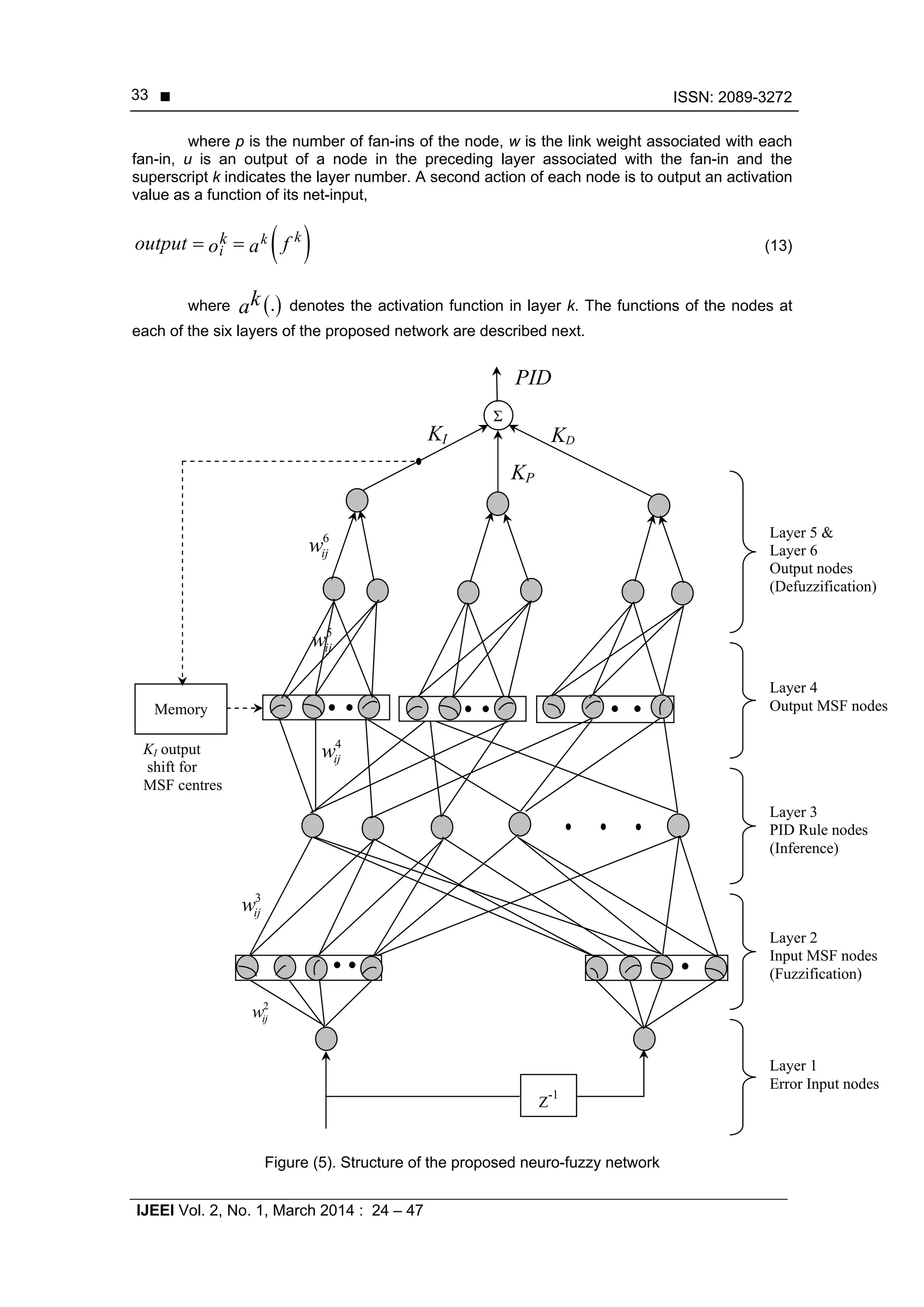
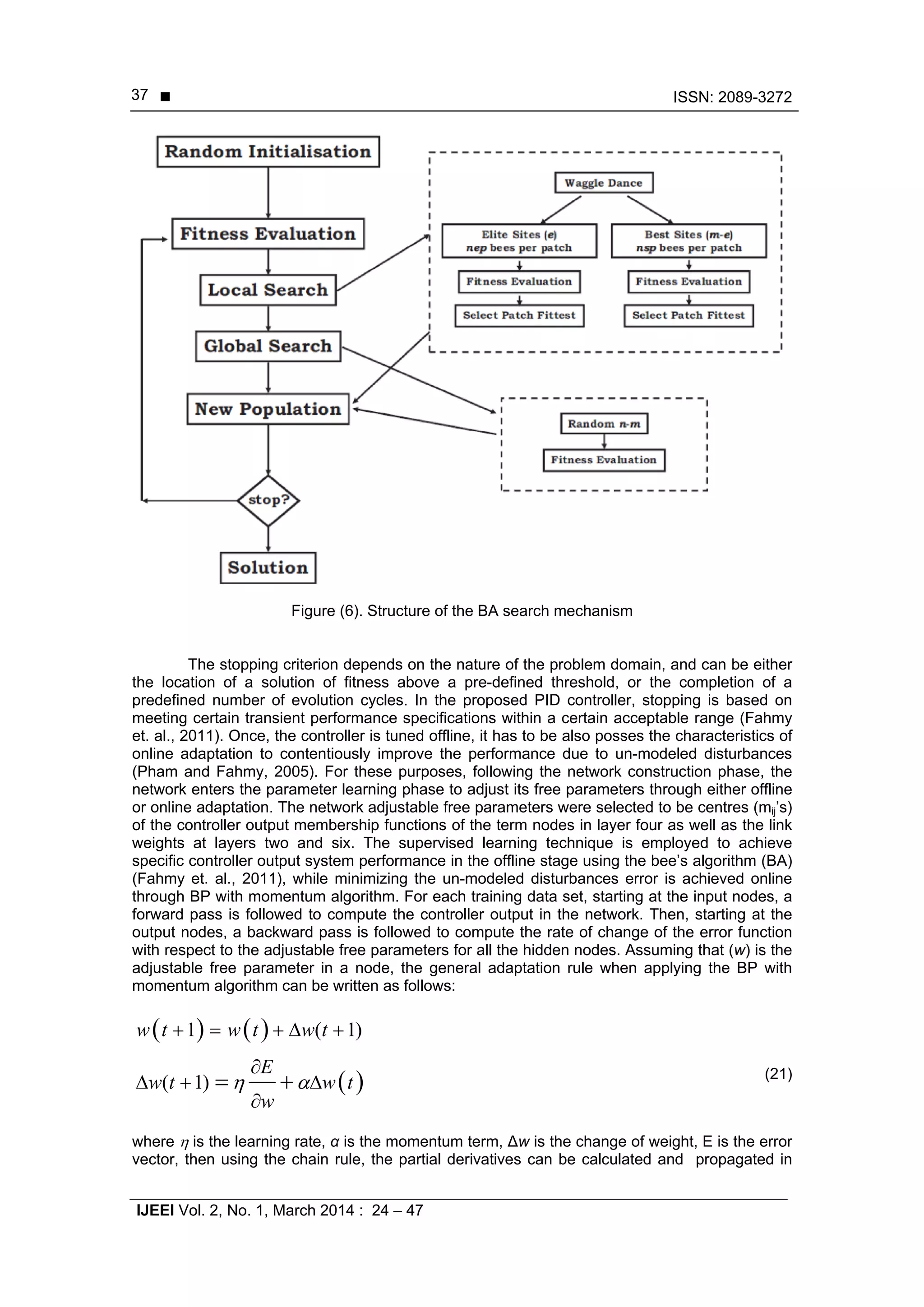
3.2. Neuro-fuzzy Network Structure
Figure (5) presents the structure of the proposed network. It consists of a six-layer feed-
forward representation of a Mamdani-model based FLS [Pham et. al., 2008. The network
structure is similar to other Mamdani-model based FFNN in the first four layers structure as in
Lin and Lee’s FFNN [Lin and Lee, 1991] and in Berenji and Khedkar’s FFNN [Berenji and
Khedkar, 1992]. The difference is in the representation of the defuzzification function, which is
represented using the last two layers (layer five and layer six) instead of one layer only. In
general, a node in any layer of the network has some finite fan-in of connections represented by
weight values from other nodes and fan-out of connections to other nodes. Associated with the
fan-in of a node is an aggregation function (f ) that serves to combine information, activation, or
evidence from other nodes. Using the same notation as in [Lin and Lee, 1991], the function
provides the net input for such a node as follows:
1 2
1 2
p
p
k
net
k k k
k k k
, ,.........., ;u u u
input f
, ,..........,w w w
 
 
 
 
(12)

 ISSN: 2089-3272
33
where p is the number of fan-ins of the node, w is the link weight associated with each
fan-in, u is an output of a node in the preceding layer associated with the fan-in and the
superscript k indicates the layer number. A second action of each node is to output an activation
value as a function of its net-input,
 kk
i
koutput fo a  (13)
where  k .a denotes the activation function in layer k. The functions of the nodes at
each of the six layers of the proposed network are described next.
Figure (5). Structure of the proposed neuro-fuzzy network
Layer 4
Output MSF nodes
Layer 5 &
Layer 6
Output nodes
(Defuzzification)
Layer 2
Input MSF nodes
(Fuzzification)
Layer 3
PID Rule nodes
(Inference)
Layer 1
Error Input nodes
KI KD
2
ijw
3
ijw
4
ijw
5
ijw
6
ijw
Memory
KI output
shift for
MSF centres
Z
-1
KP
PID
Σ

IJEEI ISSN: 2089-3272 
34
Layer 1: Nodes at layer one are input nodes, which represent input linguistic variables. Layer
one contains two nodes only (i=1, 2), which receive the current sample error value and stores
internally the previous error value. The nodes in this layer simply transmit input values directly to
the next layer. That is,
1 111
ii ii i andf fu x a   (14)
The link weights at layer one are fixed to unity.
Layer 2: Nodes at layer two are input term nodes which act as membership functions to
represent the terms of the respective error input linguistic variables. An input linguistic variable x
in a universe of discourse U is characterized by { }A,...,A,AA(x) m
x
2
x
1
x= , where A(x) is the
term set of x, that is the set of the generated membership functions (MSF) for each error input.
Layer two therefore accommodates two independent term sets, where each term set
corresponds to an error input xi and is partitioned to five (mi) terms representing input
membership functions. The function of each node j in a term set i is to calculate the degree of
membership of the input xi with respect to the membership function associated with the term set
j iA ( )x according to the specific equation of this membership function:
  
  
  
2
2
1
(15)
1
1
1
2
ij
2
ij
2
ij
2 1
ij i ij2 2
ijij
ij
2 1
ij i ij2
ij
ij
2 1
ij iij2
ij
ij
-f
=
2
=ij
f
2
=ij
f
* mw a
= and for Gaussian functionsf a e
* βw a
= and for Left sigmoidalsf a
β
e
β *w a
= and for Right sigmoidal functionsf a
β
e
σ


-
-
-
Where mij and ij are, respectively, the centre (or mean) and the width (or variance) of the
Gaussian function and ij is the characteristic value for the sigmoidal function. Hence a link
weight at layer two w2
ij can be interpreted as an adjustable free parameter of the input
membership function shape and size.
Layer 3: The nodes at layer three are the twenty-five PID rule nodes which have been
explained previously; where each node associates one term node from each term set to form a
condition part of one fuzzy rule if it is part of that rule. Hence, the rule nodes should perform the
logic min operation if the min interpretation of the sentence connective "and" between the
antecedents of a fuzzy rule is employed. Consequently in this design, the logic-min function is
replaced by the softmin function. Therefore the function of the rth
rule node using softmin can be
written as follows:
3 1
1
3 3 3
1 2 qr
33
r r
q
i
q
i
ii
i
uu e
softmin( , ,......, )f u u u
ue
and fa





 



 (16)
where r = 1,…,R, and R is the number of rules or rule nodes in layer three , q is the number of
inputs for that particular rule, ui is the ith
input to layer three, and  is an index representing the

 ISSN: 2089-3272
35
softness of the softmin function. All link weights at this layer are fixed to unity to transmit only
the membership degree of the linguistic input to the rule interpretation mechanism.
Layer 4: The nodes at layer four are output term nodes which act as membership functions to
represent the output terms of the respective l linguistic output variables (in the PID controller
case l=3). An output linguistic variable y in a universe of discourse W is characterized by
 1 2 5
y y yF(y) , ,...,F F F , where F(y) is the term set of output y, that is the set of the class
membership functions for each controller output, as explained previously, representing the
linguistic values of the controller output. Consequently layer four accommodates three
independent term sets, where each term set corresponds to individual controller output yi and is
partitioned to five terms representing output membership functions (MSF). The nodes in layer
four should perform the logic-max operation to integrate the fired rules that have the same
consequent. In the proposed neuro-fuzzy network the logic max function is replaced by the
softmax function. Therefore, the function of each term node j in the output term set i, can be
written as follows:
4 4 4 4
2 p1ij
44
ij ij
n
n
ii
i
uu e
softmax ( , ,......, ) 1f u u
ue
and fa
u




 
 
   
 
  



i 1
i 1
(17)
where p is the number of rules sharing the same consequent (the same output term node), ui is
the ith
input to layer four, and  is an index representing the softness of the softmax function.
Hence the link weights at layer four are fixed to unity.
Layer 5: The number of nodes at layer five is 2l, where l is the number of output variables (l=3),
i.e. two nodes for each output variable. The function of these two nodes is to calculate the
denominator and the numerator of an approximate form of Mean of Maxima (MOM)
defuzzification function [Saade, 1996; Runkler, 1997] for each output variable. The functions of
the two nodes of the ith
output variable are described as:
5 54 5*ij ij ni nini
= and = fa m af (18)
5 554
ij di didi
= and = fa af (19)
where
5
nif and
5
dif are respectively the node functions of the numerator and the denominator
nodes of the ith
output variable. mij is the centre (or mean) of the Gaussian function of the jth
term of the ith
output linguistic variable yi. Layer five employs 2l weight vectors, with two weight
vectors for each output variable. The first link weight vector connects the numerator node of the
ith
output to the term nodes in its term set and its components are denoted by w5
ijn . Each
component of this weight vector represents the centre (or mean) of the membership function of
the jth
term of the term set of the ith
output variable. The second link weight vector connects the
ith
output denominator node to the term nodes in its term set and its components are denoted by
w5
ijd
. Hence the link weights at layer five are fixed to unity.
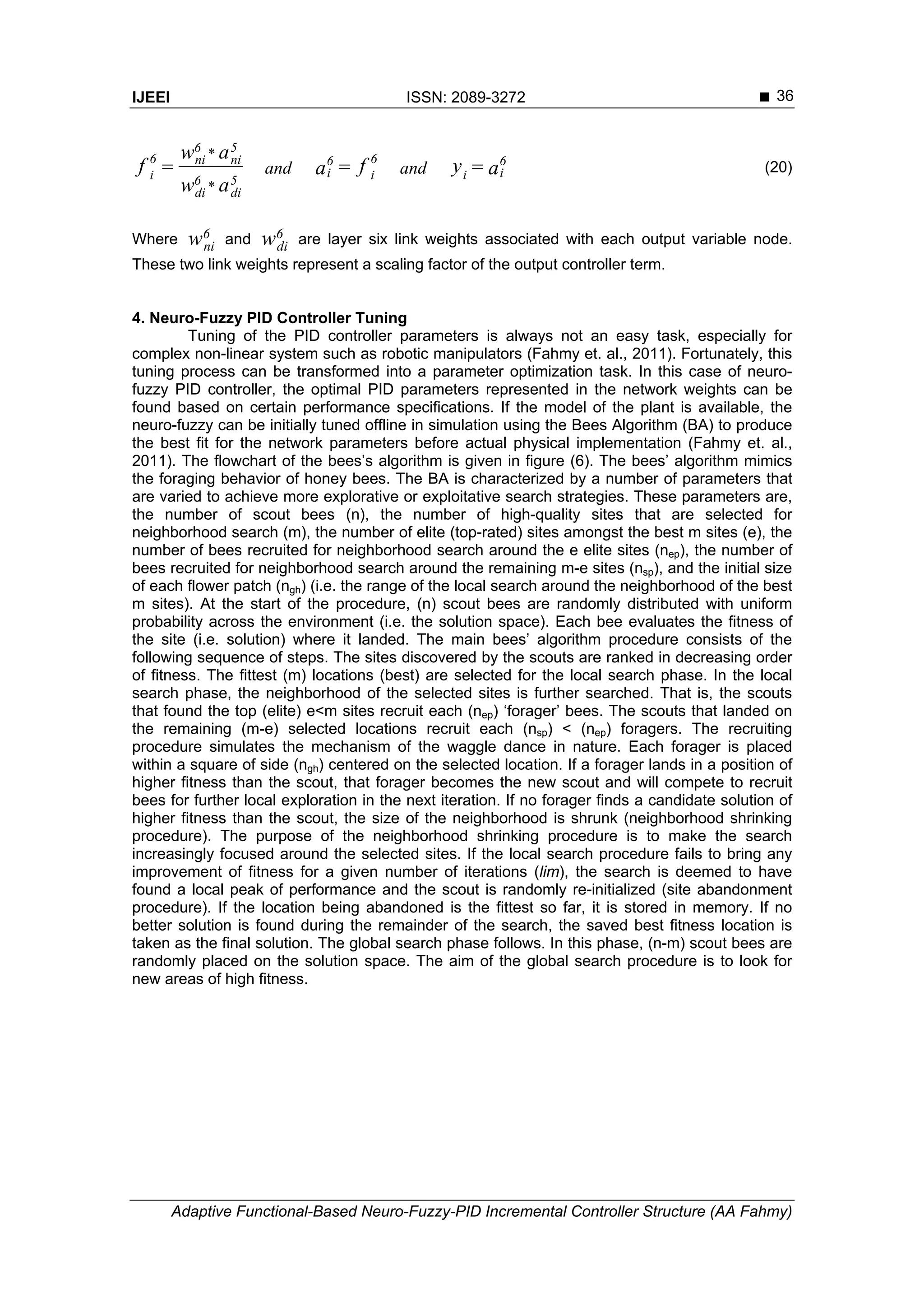
Layer 6: The nodes at layer six are defuzzification nodes. The number of nodes in layer six
equals the number of output linguistic variables (l=3). The function of the ith
node corresponding
to the ith
output variable can be written as follows:

IJEEI ISSN: 2089-3272 
36
a=yf=a
aw
aw
=f 6
ii
6
i
6
i
5
di
6
di
5
ni
6
ni6
i andand
*
*
(20)
Where w6
ni and w6
di are layer six link weights associated with each output variable node.
These two link weights represent a scaling factor of the output controller term.
4. Neuro-Fuzzy PID Controller Tuning
Tuning of the PID controller parameters is always not an easy task, especially for
complex non-linear system such as robotic manipulators (Fahmy et. al., 2011). Fortunately, this
tuning process can be transformed into a parameter optimization task. In this case of neuro-
fuzzy PID controller, the optimal PID parameters represented in the network weights can be
found based on certain performance specifications. If the model of the plant is available, the
neuro-fuzzy can be initially tuned offline in simulation using the Bees Algorithm (BA) to produce
the best fit for the network parameters before actual physical implementation (Fahmy et. al.,
2011). The flowchart of the bees’s algorithm is given in figure (6). The bees’ algorithm mimics
the foraging behavior of honey bees. The BA is characterized by a number of parameters that
are varied to achieve more explorative or exploitative search strategies. These parameters are,
the number of scout bees (n), the number of high-quality sites that are selected for
neighborhood search (m), the number of elite (top-rated) sites amongst the best m sites (e), the
number of bees recruited for neighborhood search around the e elite sites (nep), the number of
bees recruited for neighborhood search around the remaining m-e sites (nsp), and the initial size
of each flower patch (ngh) (i.e. the range of the local search around the neighborhood of the best
m sites). At the start of the procedure, (n) scout bees are randomly distributed with uniform
probability across the environment (i.e. the solution space). Each bee evaluates the fitness of
the site (i.e. solution) where it landed. The main bees’ algorithm procedure consists of the
following sequence of steps. The sites discovered by the scouts are ranked in decreasing order
of fitness. The fittest (m) locations (best) are selected for the local search phase. In the local
search phase, the neighborhood of the selected sites is further searched. That is, the scouts
that found the top (elite) e<m sites recruit each (nep) ‘forager’ bees. The scouts that landed on
the remaining (m-e) selected locations recruit each (nsp) < (nep) foragers. The recruiting
procedure simulates the mechanism of the waggle dance in nature. Each forager is placed
within a square of side (ngh) centered on the selected location. If a forager lands in a position of
higher fitness than the scout, that forager becomes the new scout and will compete to recruit
bees for further local exploration in the next iteration. If no forager finds a candidate solution of
higher fitness than the scout, the size of the neighborhood is shrunk (neighborhood shrinking
procedure). The purpose of the neighborhood shrinking procedure is to make the search
increasingly focused around the selected sites. If the local search procedure fails to bring any
improvement of fitness for a given number of iterations (lim), the search is deemed to have
found a local peak of performance and the scout is randomly re-initialized (site abandonment
procedure). If the location being abandoned is the fittest so far, it is stored in memory. If no
better solution is found during the remainder of the search, the saved best fitness location is
taken as the final solution. The global search phase follows. In this phase, (n-m) scout bees are
randomly placed on the solution space. The aim of the global search procedure is to look for
new areas of high fitness.

 ISSN: 2089-3272
37
Figure (6). Structure of the BA search mechanism
The stopping criterion depends on the nature of the problem domain, and can be either
the location of a solution of fitness above a pre-defined threshold, or the completion of a
predefined number of evolution cycles. In the proposed PID controller, stopping is based on
meeting certain transient performance specifications within a certain acceptable range (Fahmy
et. al., 2011). Once, the controller is tuned offline, it has to be also posses the characteristics of
online adaptation to contentiously improve the performance due to un-modeled disturbances
(Pham and Fahmy, 2005). For these purposes, following the network construction phase, the
network enters the parameter learning phase to adjust its free parameters through either offline
or online adaptation. The network adjustable free parameters were selected to be centres (mij’s)
of the controller output membership functions of the term nodes in layer four as well as the link
weights at layers two and six. The supervised learning technique is employed to achieve
specific controller output system performance in the offline stage using the bee’s algorithm (BA)
(Fahmy et. al., 2011), while minimizing the un-modeled disturbances error is achieved online
through BP with momentum algorithm. For each training data set, starting at the input nodes, a
forward pass is followed to compute the controller output in the network. Then, starting at the
output nodes, a backward pass is followed to compute the rate of change of the error function
with respect to the adjustable free parameters for all the hidden nodes. Assuming that (w) is the
adjustable free parameter in a node, the general adaptation rule when applying the BP with
momentum algorithm can be written as follows:
   
 
1 ( 1)
( 1)
w t w t w t
E
w t w t
w
 
    

  

  (21)
where  is the learning rate, α is the momentum term, ∆w is the change of weight, E is the error
vector, then using the chain rule, the partial derivatives can be calculated and propagated in

IJEEI ISSN: 2089-3272 
38
the network to adapt the weights [Miyamoto et. al., 1988]. Using the learning rule, the
calculations of the back-propagated errors as well as the updating of the free parameters can be
done. The adaptive rule to tune the weights of layer six is.
          6 6
6
5
6 5
1 *
*
ni ni ni
ni
net
di di
w t
a
w t w t y t ty
w a
    
 
 
  
(22)
        
 
 
6
6 6
6
6
5
2 5
*
1 *
*
ni
di di
di
di
ni
net
di
w t
w a
w t w t y t ty
w a
 

   
 
  
 
 
(23)
where 6 is the learning rate of the link weights at layer six. The error is then
propagated from layer six to the numerator and the denominator nodes at layer five. At layer
five, no adjustment is required for the link weights connected to the denominator nodes, while
an adjustment is required for the link weights 5 'nij sw which represent the centres mij’s of the
output membership functions, this adaptation has no link to the original shifting of the MSF
centre for the integral action element is performed for all controller elements. Consequently, the
adaptive rule to tune the free parameters in layer five is.
          
6
6
4
5
5
1 *
*
*ni
di
ij
netij ij ij
di
t
w
t t y t tym m m
w a
a
    
 
 
  
(24)
where 5 is the learning rate of the adjustable parameters (mij’s) at layer five. The error
is then propagated from layer five to layer four, and then from layer four to layer three. No
adjustment is required for these two layers. The error is then propagated from layer three to
layer two, where adaptation for the input membership functions is calculated as follows:
     2 2
2 2
1 ijij ij
ij
E
t t w tw w
w


   

 
 
 
(25)
where 2
ij
E
w


is calculated through error propagation chain rule, 2 is the learning rate of the link
weights in layer two and in the chain rule,
2 2
2 2
2
2 2
2
2
1 1
ij ij
ij
ij ij
ij
ij
f f
f
f f
a
for Gaussian, for L - sigmoidal, for R - sigmoidal
f
-e -e= , = =-e
e e

    
    
   
where
2
1
ij
i
f
a


is calculated as follows:
  22
2 2
2
ij ij ij
1 1 1 1i ij i ijij i i
ij
for Gaussian for L - sigmoidal for R - sigmoidal
* * mf a w a a a= ,= ,=
β βw σ
 

-

 ISSN: 2089-3272
39
  2 22 2 2
1 2
2
ij ij
1
ij ij i ijij ij ij
i ij
for Gaussian, for L - sigmoidal, for R - sigmoidal
* * mf w w a w w
= = =
β βa σ
 

-
The link weights at layer one are fixed to unity. Now, the feed-back error learning
scheme (FEL) can be applied online to tune the fuzzy-PID controller parameters online [Kawato
et. al., 1988], which combines learning and control efficiently. The objective of control is to
minimize the error between the reference signaland the plant output. If the learning part of the
architecture is disregarded, then, if the neuro-fuzzy controller is bounded, the system is stable
[Miyamura and Kimura, 2002; Terashita and Kimura, 2002]. In [Arabshahi et. al., 1992], fuzzy
control of the learning rate  is suggested. The central idea behind fuzzy control of the BP
algorithm is the implementation of the heuristics used for faster convergence in terms of fuzzy
“If-Then” rules. In this study, the fuzzy PID-like feed-back controller along with a fixed learning
rate provides the general non-linear policy of the controller and learning signal as well. It can be
seen that the proposed neuro-fuzzy PID controller is designed in a way that makes the
controller tuning achievable using any algorithm due to the contentious differentiable
membership functions selected and the differentiable fuzzification and defuzzification methods
applied in the network. The Bess Algorithm can be applied to tune the controller parameters
initially offline if the model of the plant is available, to produce a certain set-point transient
response characteristics before actual physical implementation of the controller (Fahmy et. al.,
2011). The differentiable nature of the controller structure, allow for further online tuning of the
parameters of the controller for best tracking results [Moudgal et. al., 1995, Ming-Kun et. al.,
2011].
5. Results
The proposed control system is tested by applying it to control the first two joints of a
SCARA®
type robot manipulator model with a fixed payload [Erbatur et. al., 1995, Er et. al.,
1997, Breedon et. al., 2002]. For comparison purposes, a conventional PID controller, tuned
using the Ziegler-Nichols tuning rule is used to control the robot. The controller is first tuned
using the BA to set the initial values of the controller parameters. The settings for the BA are
listed in table (5), while the setting for the BP with momentum algorithm is listed in table (6). The
error signal e (t) is defined as e (t) = r(t) − (t), and r(t) is the desired input signal. In this test,
the BA was applied for tuning the neuro-fuzzy PID controller as explained in section (4), while
the BP algorithm is applied for online tuning of the controller.
Table (5). Parameters of the BA Algorithm
Parameter Symbol Value
No. of scout bees n 30
No. of selected bees m 9
No. of elite bees e 3
Size of neighborhood ngh 9
No of sites around selected bees nsp 15
No of sites around eleite bees nep 15
Stagnation limit lim 5
Table (6). Parameters of the BP Algorithm
Parameter Symbol Value
Learning rate η 0.15
Momentum term α 0.05
Initial range for neuro-fuzzy network weights - [-1.0, 1.0]
The physical parameters of the SCARA type robot arm are given in Table (7).

IJEEI ISSN: 2089-3272 
40
Table (7). Parameters of the SCARA type robot arm
Parameter Symbol Value Unit
Link-1 Length L1 0.55 m
Link-1 CSA A1 0.15 m
2
Link-1 mass M1 1.95 kg
Link-2 Length L2 0.45 m
Link-2 CSA A2 0.11 m
2
Link-2 mass M2 1.14 kg
The objective function to be minimized for the BA was selected to be [Fahmy et. al.,
2011] :
cost 1 d 2 r 3 p 4 5 ssf w w w w wt t t M e     (26)
Where Wi ‘s are weight factors, td is delay time, tr is the rise time, tp is the peak time, M is
maximum over-shoot, and ess steady state error. The weight factors are given in table (8).
Table (8). Objective function weight values
W1 W2 W3 W4 W5
1.0 1.0 300.0 300.0 100
In the tests, the BA was used to search the initial gains of the NFPID controller to start
the PID controller gain parameters by values that achieve reasonable transient characteristics
for set-point control [ Fahmy et. al., 2011]. The objective function used is a multi-variable
objective function aiming to optimize the overall transient characteristics of the controlled
system by minimizing the elements that characterize the transient response. The objectives are
to minimize the delay time, minimize the rise time, minimize the peak time, minimize the
maximum overshoot value, and finally minimize the steady state error. The weight factors were
chosen by trial and error, with the aim of minimizing in particular the maximum overshoot, the
steady-state error, and the steady state error. For this reason, w3 to w5 are much larger w1 to w2.
In the tests, the bee’s algorithm was used to optimize the gains of the fuzzy PID controller using
the dynamic model of the robot manipulator [ Fahmy et. al., 2011]. The controller then is tested
to track link motion over repeated trajectories while the BP algorithm with momentum is applied.
Figure (8) shows the tracking results for link-1 over four consecutive cycles, while figure (9)
shows the same result for link-2. The same cycles were also tested using the conventional PID
controller and displayed on the same figures for comparison purposes. It can be observed from
the results that the proposed adaptive NFPID controller outperforms the conventional PID
controller in tracking the desired angle. Also, it can be seen that the effect of the online learning
techniques reduces the tracking error while cycles progress over time. It worth mentioning that,
the comparison with the classical PID controller is mainly to highlight the validity of the control
structure to control with complex systems. The main objectives of the trajectory test is to
highlight the capabilities of the new controller structure to adapt through online tuning to better
trajectory tracking result over time.

 ISSN: 2089-3272
41
Figure (7). Link-1 Angle in degrees tracking results
Figure (8). Link-2 Angle in degrees tracking results
6. Discussion
The contribution of this work is related to presenting a new definition of the fuzzy
differentiation, and fuzzy integration used in fuzzy systems and control. The new definition is via
introducing the idea of performing the differentiation as fuzzy function that is directly related to
the present fuzzy set membership of the error and the previous membership of the error NOT
the error value itself, rather depends on the membership function the error is related to. In this
way, the differentiation function is represented as fuzzy relation, NOT depending on the change
in error (crisp value) to be scaled in fuzzy system as represented in most previous one, two, or
three input fuzzy PID work as listed in [Hu et. al., 2001]. Moreover, the re-definition of the fuzzy
integration in this work, instead of performing the integration as fuzzy scaling to the error and
change of error with one, two, or three input fuzzy system, it is now performed as a contentious
summation of the fuzzy sets of the current error and previous sample error with continuous

IJEEI ISSN: 2089-3272 
42
shifting of the centre of the universe of discourse of the fuzzy domain itself to represent the
memory of the integration. It worth mentioning here that, this method results in re-defining the
digital differentiation and digital integration in the form of working on the fuzzy membership
functions directly. So, the control system suggested in the work is not presented as a
competitive control algorithm that outperform controller for unknown systems such as adaptive
control, robust control, predictive control etc. Rather, it is presented as a new (TRUE FUZZY)
definition for the differentiation and integration processes used in the fuzzy system with an
example of performing PID control action. For robotic tracking control where the reference and
dynamics is always changing, the inverse dynamic control is the best to be utilized, despite very
difficult to be implemented mathematically. Consequently, researcher tends to use neural
network and neuro-fuzzy systems to avoid complex mathematical formulation. In (Pham and
Anh, 2010) a gain-scheduling neural PID controller is utilized with 2-axis robotic structure for
varying the parameters of the neural PID controller to include information from the robot
dynamics. Hence, the core contribution of the paper is to introduce the new definition of the
fuzzy-PID controller as a new three fuzzy functions (fuzzy proportional, fuzzy integral and fuzzy
differential) that work directly on the membership functions that the current and previous sample
error is related to. The use of the NN structure is to implement the Fuzzy-PID controller in an
adaptive format suitable for online tuning and is not a stand alone or added item to the system,
which makes any adaptation algorithm, can be applied to tune the proposed controller either
online or off-line. The introduction of the Bees Colony is to show an example of adaptation
technique that is used previously, while the user can select the suitable algorithm to tune the
controller, even classical BP algorithm can be applied. The processing time used is dependent
on the algorithm applied for adaptation, while the non-avoidable processing time is mainly the
time used to calculate the proposed fuzzy control reactions to the error input in the form of
algebraic calculation function. The fuzzy PID controller suggested is considered as a nonlinear
model free control that possesses fixed structure that can be initially designed and then tuned to
best fit the target system while it is in operation. This characteristic and its non-linearity emulate
the classical gain scheduling and variable-structure control in their effect on the complex system
control. The effect of varying the fuzzy membership size on each P, I, or D term of the controller
is similar to varying each controller term value in classical linear PID controller, while changing
the number of controller rules is controlled by the number of membership functions in the
universe of discourse of the error domain. This directly affects the controller non-linearity and
response time, for example less number of membership functions and rules results in quicker
controller response and closer to classical linear PID controller. The optimal fuzzy model size is
normally subjected to the designer selection of the structure of the controller and its tuning
method. The frequency response of the torque result is much faster than the frequency
response of the robot mechanical time constant due to high speed computation in the virtual
domain. NI the proposed work, the main target is to demonstrate the tracking convergence to
the desired trajectory, while the learning process of the controller proceeds. The detailed initial
tuning process and variations of the PID controller gains is described in the author previous
work [Fahmy et. al., 2011], while the scope of the work is to highlight the new controller design
structure, online learning, and tracking capabilities.
7. Conclusion
This paper proposed a new adaptive functional based adaptive neuro-fuzzy-PID
(NFPID) controller that can be tuned offline to set the initial parameters using the BA to achieve
certain transient performance specifications based on the system model. The proposed
controller differential structure permits also for online adaptation of the controller that can used
to obtain another set of parameters that achieve better tracking and eliminate un-modelled
disturbances effect on the system performance for the problem of trajectory control of robotic
manipulators. The scope contribution of the paper is not to introduce an outperforming controller
for the MIMO robotic structure presented in the paper, rather it is to introduce a new definition
for fuzzy PID controller and a new representation that is simple and effective to do the control
job with the capability for further tuning online while the system is operation. So, the choice of
the robotic structure as a test bed for the controller is for demonstration purposes of the
controller capabilities not to claim its outperformance over the classical PID control or other
controller structure used for robotic manipulation control. The use of a fixed payload on the

 ISSN: 2089-3272
43
robotic structure is to highlight the idea that the controller, despite the main contribution is its
new definition for the fuzzy integral and fuzzy differential, it is still can be adapted to cope with
variation in a nonlinear system results from changing structure, while a fixed gain controller,
despite could achieve good control performance in the fixed robot structure, it could easily
deviate the trajectory considerably when the structure is changed by attached load. This new
adaptive neuro-fuzzy-PID (NFPID) controller was applied to control the first two links of a
SCARA® type robot manipulator model over pre-planned joint-trajectories while carrying a fixed
payload. The results showed that the method was successful and applicable for robotic
manipulators control.
References
[1] Ahn KK & Anh HPH. Identification of the pneumatic artificial muscle manipulators by MGA-based
nonlinear NARX fuzzy model. IFAC Journal of Mechatronics. 2009; 19(1): 106–133.
[2] Anh, Ho Pham Huy. Online tuning scheduling MIMO neural PID control of the 2-axes pneumatic
artificial muscle (PAM) robot arm. Expert Systems with applications. 2010; 37(9): 6547-6560.
[3] Arabshahi P, Choi JJ, Marks RJ, and Caudell TP. Fuzzy Control of Backpropagation, IEEE
International Conference on Fuzzy Systems, 8-12 March 1992, San Diego, California, USA. 1992:
967-972.
[4] Bao-Gang H, George KIM, and Raymond GG. A systematic study of fuzzy PID controllers- Function-
Based Evaluation Approach. IEEE transactions on fuzzy systems. 2001; 9(5).
[5] Berenji HR and Khedkar P. Learning and Tuning Fuzzy Logic Controllers Through Reinforcements.
IEEE Transactions on Neural Networks. 1992; 3(5): 724-740.
[6] Breedon PJ, Sivayoganathan K, Balendran V, and Al-Dabass D. Multi-Axis Fuzzy Control and
Performance Analysis for an Industrial Robot. Proceedings of the IEEE International Conference on
Fuzzy Systems, 12-17 May 2002, Honolulu, HI, USA. 2002; 1: 500-505.
[7] Er MJ, Yap SM, Yeaw CW, and Luo FL. A Review of Neural-Fuzzy Controllers for Robotic
Manipulators, Thirty-Second IAS Annual Meeting, IEEE Industry Applications Conference, 5-9
October 1997, New Orleans, Los Anglos, USA. 1997; 2: 812-819.
[8] Erbatur K, Kaynak O, and Rudas I. A Study of Fuzzy Schemes for Control of Robotic Manipulators.
IECON Twenty-First IEEE International Conference on Industrial Electronics, Control, and
Instrumentation, 6-10 November 1995, Orlando, Florida, USA. 1995; 1: 63-68.
[9] Estevez PA and Nakano R. Hierarchical Mixture of Experts and Max-Min Propagation Neural
Networks. IEEE International Conference on Neural Networks, 27 November -1 December 1995,
Perth, WA, Australia. 1995: 651-565.
[10] Fahmy AA, Abdel Ghany AM. Neuro-fuzzy inverse model control structure of robotic manipulators
utilized for physiotherapy applications. Proceeding of Ain Shams Engineering Journal. 2013; 2090-
4479.
[11] Fahmy AA, Kalyoncu M, Castellani M. Automatic design of control systems for robot manipulators
using the bees algorithm. Proceeding of the Institute of Mechanical Engineers, Part I: Journal of
Systems and Control Engineering. 2011; I.
[12] Huang Y and Yasunobu S. A General Practical Design Method for Fuzzy PID Control from
Conventional PID Control. The Ninth IEEE International Conference on Fuzzy Systems. 2000; 2.
[13] Karasakal O, Yesil E, Guzelkaya M, and Eksin I. Implementation of a new self-tuning fuzzy PID
controller on PLC. Turkish Journal of Electrical Engineering. 2005; 13(2): 277-286.
[14] Kawato M, Uno Y, Isobe M, and Suzuki R. Hierarchical Neural Network Model for Voluntary
Movement with Application to Robotics. IEEE Control Systems Magazine. 1988; 8(2): 8-15.
[15] Lee CC. Fuzzy Logic in Control Systems Fuzzy Logic controller Part I. IEEE Transactions on Systems,
Manufacturing, and Cybernetics. 1990; 20(2): 404-418.
[16] Lee CC. Fuzzy Logic in Control Systems Fuzzy Logic controller Part II. IEEE Transactions on
Systems, Manufacturing, and Cybernetics. 1990; 20(2): 419-435.
[17] Lin CT and Lee CSG. Neural Network-Based Fuzzy Logic Control and Decision System. IEEE
Transactions on Computers. 1991; 40(12): 1320-1336.
[18] Mann G, Bao-Gang Hu, and Gosine R. Analysis of direct action fuzzy PID controller structures. IEEE
Transactions on Systems, Man, and Cybernetics, Part B: Cybernetics. 1999; 29(3).
[19] Ming-Kun C, Jeih-Jang L, Ming-Lun C. T-S fuzzy model-based tracking control of a one-dimentional
manipulator actuated by pneumatic artificial muscles. Control Engineering Practice. 2011; 19: 1442-
1449.
[20] Miyamoto H, Kawato M, Setoyama T, and Suzuki R. Feedback-Error Learning Neural Network for
Trajectory Control of Robotic Manipulator. Neural Networks. 1988; 1(3): 251-265.
[21] Miyamura A and Kimura H. Stability of Feedback Error Learning Scheme.
Systems & Control Letters. 2002; 45(4): 303-316.

IJEEI ISSN: 2089-3272 
44
[22] Moudgal VG, Kwong WA, and Passino KM. Fuzzy Learning Control for a Flexible-Link Robot. IEEE
Transactions on Fuzzy Systems. 1995; 3(2): 199-210.
[23] Nauck D and Kruse R. A fuzzy neural network learning fuzzy control rules and membership functions
by fuzzy error back propagation. IEEE International Conference on Neural Networks. 1993: 1022-
1027.
[24] Pedrycz W. Fuzzy Control and Fuzzy Systems. John Wiley & Sons Publications Incorporation,
Taunton, NewYork. 1993.
[25] Petrov M, Ganchev I, and Taneva A. Fuzzy PID control of nonlinear plants. First International IEEE
Symposium Intelligent Systems. 2002.
[26] Pham DT and Fahmy AA. Neuro-fuzzy modelling and control of robot manipulators for trajectory
tracking. Proceedings of the 16th IFAC World Congress, 2005, Czech Republic. 2005; 16(1): 415-429.
[27] Pham DT, Fahmy AA, Eldukhri EE. Adaptive fuzzy neural network for inverse modeling of robot
manipulators, Proceedings of the 17th IFAC World Congress, 2008, Seoul, Korea. 2008: 5308-5313.
[28] Runkler TA. Selection of Appropriate Defuzzification Methods Using Application Specific Properties.
IEEE Transactions on Fuzzy Systems. 1997; 5(1): 72-79.
[29] Saade JJ. A Unifying Approach to Defuzzification and Comparison of the Outputs of Fuzzy
Controllers. IEEE Transactions on Fuzzy Systems. 1996; 4(3): 227-237.
[30] Shankir Y. Fuzzy Logic Systems and Fuzzy Neural Networks for Dynamic Systems Modelling and
Control, Ph.D. Thesis, University of Wales, Cardiff School of Engineering, Cardiff University, UK.
2001.
[31] Sheroz Khan, A Adam, AHM Zahirul Alam, Mohd Rafiqul Islam, and Othman O Khalifa. Rule-Based
fuzzy logic controller with adaptable reference. International journal of electrical and computer
engineering. 2008; 3(5).
[32] Shing J and Jang R. ANFIS: Adaptive-Network-Based Fuzzy Inference System. IEEE Transactions on
Systems, Man., and Cybernetics. 1993; 23(3).
[33] Sinthipsomboon K, Hunsacharoonroj I, Khedari J, Pongaen W, and Pratumsuwan P. A hybrid of fuzzy
and fuzzy self-tuning PID controller for servo electro-hydraulic system. 6th IEEE Conference on
Industrial Electronics and Applications (ICIEA). 2011.
[34] Takagi T and Sugeno M. Fuzzy Identification of Systems and Its Applications to Modelling and
Control. IEEE Transactions on Systems, Manufacturing, and Cybernetics. 1985; SMC-15(1): 116-132.
[35] Tang W, Chen G and Lu R. A Modified Fuzzy PI Controller for a Flexible-Joint Robot Arm with
Uncertainties. Fuzzy Sets and Systems. 2001; 118(1, 16): 109-119.
[36] Terashita J and Kimura H. Robustness of Feedback Error Learning Method with Time Delay.
Proceedings of the 41
st
SICE/IEEE Annual Conference, 5-7 August 2002, Tokyo, Japan. 2002; 4:
2240-2244.
[37] Ying H. The Simplest Fuzzy Controllers Using Different Inference Methods are Different Non-linear
Proportional-Integral-Controllers with Variable Gains. Automatica. 1993; 29(6): 1579-1589.
[38] Ying H, Siler W, and Buckley JJ. Fuzzy Control Theory: A Non-linear Case. Automatica. 1990; 26(3):
513-520.
[39] Yuan F, Feldkamp LA, Davis LI, Jr, and Puskorius GV. Training a Hybrid Neural-Fuzzy System,
IEEE/IJCNN International Joint Conference on Neural Networks, 7-11 June 1992, Baltimore, MD,
USA. 1992; 2: 739-744.
[40] Zhang X, Hang CC, Tan S, and Wang PZ. The Min-Max Function Differentiation and Training of Fuzzy
Neural Networks. IEEE Transactions on Neural Networks. 1996; 7(5): 1139-1150.
Appendix (A): SCARA Robot Dynamics
The equations of motion can be described by a set of differential or difference equations. The
equation set consists of two parts, the kinematics equations and the dynamic equation. Robot
arm kinematics deals with the geometry of robot arm motion as a function of time (position,
velocity, and acceleration) without reference to the forces and moments that cause this motion,
while the dynamics of robot is the study of motion with regard to forces and torques.
In robotics manipulators, there are two methodologies used for dynamic modeling.
a) Newton-Euler formulation.
b) Lagrangian formulation.
An analytical approach based on the Lagrange's energy function, known as Lagrange- Euler
method, results in a dynamic solution that is simple and systematic. In this method, the kinetic
energy (K) and the potential energy (P) are expressed in terms of joint motion trajectories. The
resulting differential equations then provide the forces (torques) which drive the robot. Closed
form equations result in a structure that is very useful for robot control design and also
guarantee a solution. The dynamics of n-link manipulators are conveniently described by
Lagrangian dynamics. In the Lagrangian approach, the joint variables, q = (q
1
; . ... .; q
n
)T
, serve

 ISSN: 2089-3272
45
as a suitable set of generalized coordinates. The kinetic energy is a quadratic function of the
vector
.
q of the form:
K
.
)(
.
2
1..
)(
2
1
1,
qqDTqjqiqqijd
n
ji


(A.1)
Where the nxn "inertia matrix" D(q) is symmetric and positive definite for each q. The
gravitational potential energy P=P(q) is independent of
.
q. The Euler-Lagrange equations for
such a system can be derived as follows. Since
L = K – P = j
.
qi
.
q)q(ijd
n
j,i

12
1
- P (q (A.2)
where L is the Lagrangian then the dynamic equations of an n-joint robotic manipulator
described by Lagrange's equations can be expressed as:
D
..
q)q( +C(q,
.
q )
.
q +G(q)+B(
.
q ) = (A.3)
where q is the generalized coordinates of the robot arm,
.
i
q is the first derivative of q
i
; D(q) is
the symmetric, bounded, positive-definite inertia matrix; vector C(q,
.
q )
.
q presents the
centrifugal and Coriolis torque; G(q) , B(
.
q ) and  represent the gravitational torque, friction, and
applied joint torque, respectively.
D(q) (nxn matrix) expressed as:
    







n
k
k
k
Tkk
k
Tk
qBqDqBqAmqAqD
1
)()()()()()( (A.4)
Where Ak
and Bk
represent 3xn Jacobian submatrices, mk is the mass of link k and Dk is the nxn
link inertia tensor which depends on q. The equation of velocity coupling vector C(q,
.
q ,) is:
C(q,
.
q ) = jk
n
k kj
i
kjk
n
k
i
kk qqqCqqC
..
)(
.
)(  
  1
2
1
(A.5)
The equation of gravity loading vector (nx1) is:
)q(A imgqG
3
1k
n
ij
j
kjki
)(  
 

(A.6)
and the frictional force model for joint k is expressed as:

IJEEI ISSN: 2089-3272 
46
Bk(
.
q ) = k
v
k qb
.
sgn 





 e
f
bbbq
d
k
s
k
d
kk )()
.
( (A.7)
where: f =
ε
.
q
k

, b
v
k represent the coefficient of viscous friction, b
d
k is the coefficient of
dynamic friction, and b
s
k is the coefficient of static friction for joint k and  is a small positive
parameter. The dynamic equation derived by using the Euler- Lagrangian method for the first
two arms of the SCARA configuration will be as follows [6]:
1st joint:
1 = [(
3
m1 + m2)
2
1a + m2 a1a2 C2 +
3
m2 2
2a ]
..
1
q
+[
2
m2 a1a2C2+
3
m2 2
2a ]
..
2
q -m2a1a2S2( 1
.
q 2
.
q +
2
2
2
.
q )+b1( 1
.
q ) (A.8)
2nd joint:
2=[
2
m2 a1a2C2+
3
m2 2
2a ]
..
1
q +
3
m2 2
2a
..
2
q +
2
m2 a1a2S2
2
1
.
q +b2( 2
.
q ) (A.9)
Where mi is the mass and ai is the length of link i, C and S represent the cos(q) and sin(q),
respectively. Let the state defines as xT
=[qT
, vT
], where v=q
.
. Since n=2, the manipulator inertia
tensor is a symmetric 2x2 matrix. From the coefficients of the joint accelerations, the distinct
components of D(q) are:
D11(q)= (
3
m1 + m2) 2
1a + m2a1a2 C2 +
3
m2 2
2a (A.10)
D12(q) =
2
m2 a1a2 C2 +
3
m2 2
2a (A.11)
Because D(q) is symmetric then
D12(q) = D21 (q) (A.12)
D22 (q)=
3
m2 2
2a (A.13)
(q)= D11 D22 - D12 D21 (A.14)
1
.
q = v1, 2
.
q = v2 (A.15)

 ISSN: 2089-3272
47
1
.
v =
)( q
1
[D22(q) {1+a1a2S2m2(v1v2+
2
1
v2
2
)- b1( 1
.
q )}
- D12(q) {2 -
2
2m
a1a2S2 v1
2
- b2( 2
.
q )}] (A.16)
2
.
v =
)(q
1
[- D21(q) {1+a1a2S2m2(v1v2+
2
1
v2
2
)- b1( 1
.
q )}
+ D11(q) {2 -
2
m2 a1a2S2 v1
2
- b2( 2
.
q )}] (A.17)

Adaptive Functional-Based Neuro-Fuzzy-PID Incremental Controller Structure

Recommended

Recommended

More Related Content

What's hot

What's hot (18)

Similar to Adaptive Functional-Based Neuro-Fuzzy-PID Incremental Controller Structure

Similar to Adaptive Functional-Based Neuro-Fuzzy-PID Incremental Controller Structure (20)

More from ijeei-iaes

More from ijeei-iaes (20)

Recently uploaded

Recently uploaded (20)

Adaptive Functional-Based Neuro-Fuzzy-PID Incremental Controller Structure