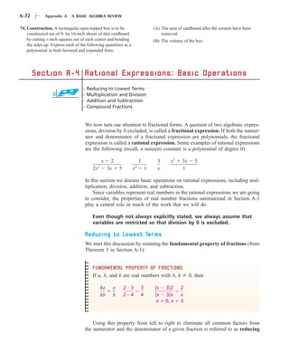
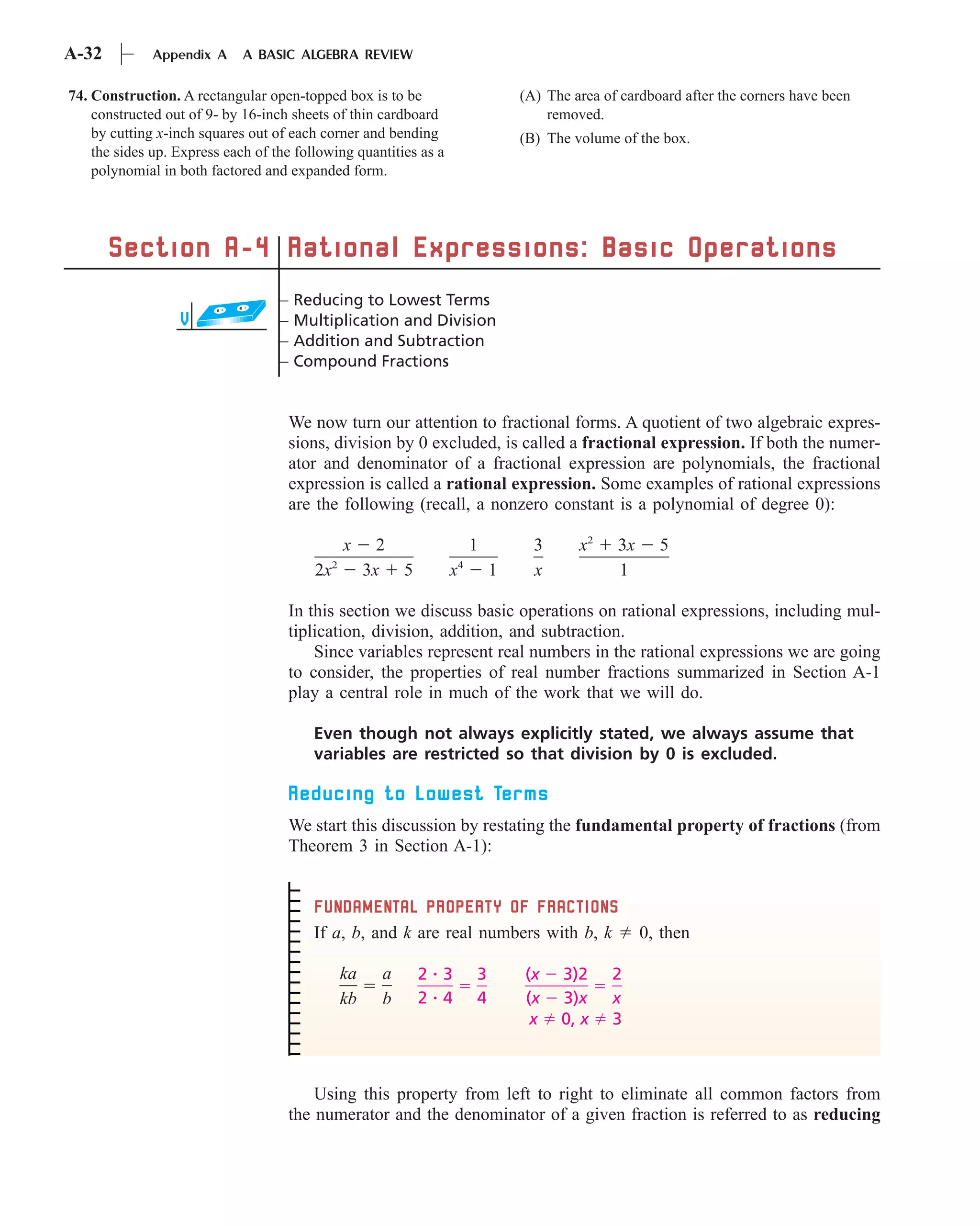
This document discusses operations on rational expressions, including: 1) Reducing rational expressions to lowest terms by dividing the numerator and denominator by their greatest common factor. 2) Multiplying rational expressions follows the same rules as multiplying fractions - the numerators are multiplied and the denominators are multiplied. 3) Dividing rational expressions follows the same rules as dividing fractions - the expression is written as the first rational expression over the second.

1. A-32 Appendix A A BASIC ALGEBRA REVIEW
74. Construction. A rectangular open-topped box is to be (A) The area of cardboard after the corners have been
constructed out of 9- by 16-inch sheets of thin cardboard removed.
by cutting x-inch squares out of each corner and bending (B) The volume of the box.
the sides up. Express each of the following quantities as a
polynomial in both factored and expanded form.
Section A-4 Rational Expressions: Basic Operations
Reducing to Lowest Terms
Multiplication and Division
Addition and Subtraction
Compound Fractions
We now turn our attention to fractional forms. A quotient of two algebraic expres-
sions, division by 0 excluded, is called a fractional expression. If both the numer-
ator and denominator of a fractional expression are polynomials, the fractional
expression is called a rational expression. Some examples of rational expressions
are the following (recall, a nonzero constant is a polynomial of degree 0):
x 2 1 3 x2 3x 5
2 4
2x 3x 5 x 1 x 1
In this section we discuss basic operations on rational expressions, including mul-
tiplication, division, addition, and subtraction.
Since variables represent real numbers in the rational expressions we are going
to consider, the properties of real number fractions summarized in Section A-1
play a central role in much of the work that we will do.
Even though not always explicitly stated, we always assume that
variables are restricted so that division by 0 is excluded.
Reducing to Lowest Terms
We start this discussion by restating the fundamental property of fractions (from
Theorem 3 in Section A-1):
FUNDAMENTAL PROPERTY OF FRACTIONS
If a, b, and k are real numbers with b, k 0, then
ka a 2 3 3 (x 3)2 2
kb b 2 4 4 (x 3)x x
x 0, x 3
Using this property from left to right to eliminate all common factors from
the numerator and the denominator of a given fraction is referred to as reducing

2. A-4 Rational Expressions: Basic Operations A-33
a fraction to lowest terms. We are actually dividing the numerator and denom-
inator by the same nonzero common factor.
Using the property from right to left—that is, multiplying the numerator and
the denominator by the same nonzero factor—is referred to as raising a fraction
to higher terms. We will use the property in both directions in the material that
follows.
We say that a rational expression is reduced to lowest terms if the numera-
tor and denominator do not have any factors in common. Unless stated to the con-
trary, factors will be relative to the integers.
EXAMPLE Reducing Rational Expressions
1 Reduce each rational expression to the lowest terms.
x2 6x 9 (x 3)2 Factor numerator and denomina-
(A) 2 tor completely. Divide numerator
x 9 (x 3)(x 3)
and denominator by (x 3); this is
x 3 a valid operation as long as x 3
x 3 and x 3.
1
x3 1 (x 1)(x2 x 1) Dividing numerator and denomina-
(B) 2 tor by (x 1) can be indicated by
x 1 (x 1)(x 1)
1 drawing lines through both
(x 1)s and writing the resulting
quotients, 1s.
x2 x 1
x 1 and x 1
x 1
MATCHED PROBLEM Reduce each rational expression to lowest terms.
1 (A)
6x2 x 2
(B)
x4 8x
2x2 x 1 3x3 2x2 8x
EXAMPLE Reducing a Rational Expression
2 Reduce the following rational expression to lowest terms.
6x5(x2 2)2 4x3(x2 2)3 2x3(x2 2)2[3x2 2(x2 2)]
8
x x8
1
2x3(x2 2)2(x2 4)
x8
x5
2(x2 2)2(x 2)(x 2)
x5

3. A-34 Appendix A A BASIC ALGEBRA REVIEW
MATCHED PROBLEM Reduce the following rational expression to lowest terms.
2 6x4(x2 1)2 3x2(x2 1)3
x6
Remember to always factor the numerator and denominator first, then
CAUTION divide out any common factors. Do not indiscriminately eliminate terms
that appear in both the numerator and the denominator. For example,
1
2x3 y2 2x3 y2
2x3 1
y2 y2
1
Since the term y2 is not a factor of the numerator, it cannot be elimi-
nated. In fact, (2x3 y2)/y2 is already reduced to lowest terms.
Multiplication and Division
Since we are restricting variable replacements to real numbers, multiplication and
division of rational expressions follow the rules for multiplying and dividing real
number fractions (Theorem 3 in Section A-1).
MULTIPLICATION AND DIVISION
If a, b, c, and d are real numbers with b, d 0, then:
a c ac 2 x 2x
1.
b d bd 3 x 1 3(x 1)
a c a d 2 x 2 x 1
2. c 0
b d b c 3 x 1 3 x
Explore/Discuss Write a verbal description of the process of multiplying two fractions. Do
the same for the quotient of two fractions.
1

4. A-4 Rational Expressions: Basic Operations A-35
EXAMPLE Multiplying and Dividing Rational Expressions
3 Perform the indicated operations and reduce to lowest terms.
5x2 1 1 Factor numera-
10x y 3
x 2
9 10x3y (x 3)(x 3) tors and denom-
(A) inators; then
3xy 9y 4x2 12x 3y(x 3) 4x(x 3)
divide any nu-
3 1 2 1 merator and any
5x2 denominator
6 with a like com-
mon factor.
1
4 2x 2(2 x) 1 x 2
(B) (x 2) x 2 is the same as .
4 4 x 2 1
2
1
2 x (x 2) b a (a b),
a useful change in
2(x 2) 2(x 2) some problems.
1
1
2
2x3 2x2y 2xy2 x3 y3
(C)
x y xy3
3
x2
2xy y2
2 1 1
2x(x2 xy y2) (x y)2
xy(x y)(x y) (x y)(x2 xy y2)
y 1 1 1
2
y(x y)
MATCHED PROBLEM Perform the indicated operations and reduce to lowest terms.
3 (A)
12x2y3
2
y2 6y 9
3 2
(B) (4 x)
x2 16
2xy 6xy 3y 9y 5
3 3 3 2 2 3
m n mn mn mn
(C) 2 2 3 2 2 3
2m mn n 2m n mn

5. A-36 Appendix A A BASIC ALGEBRA REVIEW
Addition and Subtraction
Again, because we are restricting variable replacements to real numbers, addition
and subtraction of rational expressions follow the rules for adding and subtract-
ing real number fractions (Theorem 3 in Section A-1).
ADDITION AND SUBTRACTION
For a, b, and c real numbers with b 0:
a c a c x 2 x 2
1.
b b b x 3 x 3 x 3
a c a c x x 4 x (x 4)
2.
b b b 2xy 2 2xy 2 2xy 2
Thus, we add rational expressions with the same denominators by adding or
subtracting their numerators and placing the result over the common denomina-
tor. If the denominators are not the same, we raise the fractions to higher terms,
using the fundamental property of fractions to obtain common denominators, and
then proceed as described.
Even though any common denominator will do, our work will be simplified
if the least common denominator (LCD) is used. Often, the LCD is obvious, but
if it is not, the steps in the box describe how to find it.
THE LEAST COMMON DENOMINATOR (LCD)
The LCD of two or more rational expressions is found as follows:
1. Factor each denominator completely.
2. Identify each different prime factor from all the denominators.
3. Form a product using each different factor to the highest power that
occurs in any one denominator. This product is the LCD.
EXAMPLE Adding and Subtracting Rational Expressions
4 Combine into a single fraction and reduce to lowest terms.
3 5 11 4 5x
(A) (B) 1
10 6 45 9x 6y2
x 3 x 2 5
(C) 2
x 6x 9 x2 9 3 x
Solutions (A) To find the LCD, factor each denominator completely:
10 2 5
6 2 3 LCD 2 32 5 90
45 32 5

6. A-4 Rational Expressions: Basic Operations A-37
Now use the fundamental property of fractions to make each denominator
90:
3 5 11 9 3 15 5 2 11
10 6 45 9 10 15 6 2 45
27 75 22
90 90 90
27 75 22 80 8
90 90 9
9x 32x
(B) LCD 2 32xy2 18xy2
6y2 2 3y2
4 5x 2y2 4 3x 5x 18xy2
1
9x 6y2 2y2 9x 3x 6y2 18xy2
8y2 15x2 18xy2
18xy2
x 3 x 2 5 x 3 x 2 5
(C)
x2 6x 9 x2 9 3 x (x 3)2 (x 3)(x 3) x 3
5 5 5 We have again used
Note: the fact that
3 x (x 3) x 3
a b (b a).
The LCD (x 3)2(x 3). Thus,
(x 3)2 (x 3)(x 2) 5(x 3)(x 3)
(x 3)2(x 3) (x 3)2(x 3) (x 3)2(x 3)
(x2 6x 9) (x2 x 6) 5(x2 9) Be careful of sign
(x 3)2(x 3) errors here.
x2 6x 9 x2 x 6 5x2 45
(x 3)2(x 3)
5x2 7x 30
(x 3)2(x 3)
MATCHED PROBLEM Combine into a single fraction and reduce to lowest terms.
4 5 1 6 1 2x 1 3
(A) (B)
28 10 35 4x2 3x3 12x
y 3 y 2 2
(C)
y2 4 y 2
4y 4 2 y

7. A-38 Appendix A A BASIC ALGEBRA REVIEW
16
Explore/Discuss
What is the value of 4 ?
2
2 What is the result of entering 16
What is the difference between 16
4
(4
2 on a calculator?
2) and (16 4) 2?
How could you use fraction bars to distinguish between these two cases
16
when writing 4 ?
2
Compound Fractions
A fractional expression with fractions in its numerator, denominator, or both is
called a compound fraction. It is often necessary to represent a compound frac-
tion as a simple fraction—that is (in all cases we will consider), as the quotient
of two polynomials. The process does not involve any new concepts. It is a mat-
ter of applying old concepts and processes in the right sequence. We will illus-
trate two approaches to the problem, each with its own merits, depending on the
particular problem under consideration.
EXAMPLE Simplifying Compound Fractions
5 Express as a simple fraction reduced to lowest terms.
2
1
x
4
1
x2
Solution Method 1. Multiply the numerator and denominator by the LCD of all frac-
tions in the numerator and denominator—in this case, x2. (We are multiplying by
1 x2/x2).
2 2 1
x2 1 x2 x2
x x 2x x2 x(2 x)
4 4 4 x2 (2 x)(2 x)
x2 2 1 x2 2 x2
x x 1
x
2 x

8. A-4 Rational Expressions: Basic Operations A-39
Method 2. Write the numerator and denominator as single fractions. Then treat as
a quotient.
2 2 x 1 x
1
x x 2 x 4 x2 2 x x2
4 4 x2 x x2 x (2 x)(2 x)
1
x2 2
x 1 1
x
2 x
MATCHED PROBLEM Express as a simple fraction reduced to lowest terms. Use the two methods
5 described in Example 5.
1
1
x
1
x
x
EXAMPLE Simplifying Compound Fractions
6 Express as a simple fraction reduced to lowest terms.
y x
x2 y2
y x
x y
Solution Using the first method described in Example 5, we have
y x y x 1
x2y2 x2y2 x2y2
x2 y2 x2 y2 y3 x3 (y x)(y2 xy x2)
y x y x xy3 x3y xy(y x)(y x)
x2y2 x2y2 x2y2
x y x y 1
y2 xy x2
xy(y x)
MATCHED PROBLEM Express as a simple fraction reduced to lowest terms. Use the first method
6 described in Example 5.
a b
b a
a b
2
b a

9. A-40 Appendix A A BASIC ALGEBRA REVIEW
Answers to Matched Problems
3x 2 x2 2x 4 3(x2
1)2(x 1)(x 1) 5
1. (A) (B) 2. 3. (A) 2x (B) (C) mn
x 1 3x 4 x4 x 4
1 3x2 5x 4 2y2
9y 6 1 a b
4. (A) (B) (C) 5. 6.
4 12x3 ( y 2)2( y 2) x 1 a b
EXERCISE A-4 B
Problems 21–26 are calculus-related. Reduce each fraction to
lowest terms.
A
6x3(x2 2)2 2x(x2 2)3
21.
In Problems 1–20, perform the indicated operations and x 4
reduce answers to lowest terms. Represent any compound 4 2
fractions as simple fractions reduced to lowest terms. 4x (x 3) 3x2(x2 3)2
22. 6
x
d5 d2 a d5 d2 a
1. 2. 2x(1 3x)3 9x2(1 3x)2
3a 6a2 4d 3 3a 6a2 4d 3 23.
(1 3x)6
2y 1 y x2 x 1
3. 4. 2x(2x 3)4 8x2(2x 3)3
18 28 42 12 18 30 24.
(2x 3)8
3x 8 2x 1 5 4m 3 3 2m 1
5. 6. 2x(x 4)3 3(3 x2)(x 4)2
4x2 x3 8x 18m3 4m 6m2 25.
(x 4)6
2x2 7x 3 x2 9
7. (x 3) 8. (x2 x 12) 3x2(x 1)3 3(x3 4)(x 1)2
4x2 1 x2 3x 26.
(x 1)6
m n m2 mn
9.
m2 n2 m 2
2mn n2 In Problems 27–40, perform the indicated operations and
x 2
6x 9 x 2
2x 15 reduce answers to lowest terms. Represent any compound
10. fractions as simple fractions reduced to lowest terms.
x2 x 6 x2 2x
y 1 2
1 1 27.
11. 2 2 2 2 y2 y 2 y2 5y 14 y2 8y 7
a b a 2ab b
2
x x 1 1
3 2 28.
12. x2 2x 1 3x 3 6
x2 1 x2 2x 1
9 m2 m 2
m 1 x 1 29.
13. m 3 14. 1 m2
5m 6 m 3
m 2 x 1
2 x x2 4x 4
5 2 3 2 30.
15. 16. 2x x2 x2 4
x 3 3 x a 1 1 a
x 7 y 9
2 1 2y 31.
17. ax bx by ay
y 3 y 3 y2 9
c 2 c 2 c
2x 1 1 32.
18. 2 2 5c 5 3c 3 1 c
x y x y x y
2 2
x 16 x 13x 36
y2 3 33.
1 1 2x2 10x 8 x3 1
x2 x
19. 20.
y 9 x3 y3 y x2 xy y2
1 x 34. 3
x x y x y y2

10. A-5 Integer Exponents A-41
x2 xy x2 y2 x2 2xy y2 (x h)3 x3
35. 48. (x 1)3 x3 3x2 3x 1
xy y2 x 2
2xy y 2
xy 2
xy 2 h
x2 xy x2 y2 x2 2xy y2 x2 2x x2 2x x 2
36. 49. 2
x 2 1
xy y2 x 2
2xy y2
xy 2
xy 2 x x 2 x2 x 2
x 1 4 2 x 3 2x 2 x 3 1
37. 50.
x2 16 x 4 x 4 x 1 x2 1 x2 1 x 1
2 2 2
3 1 x 4 2x x 2x x 2x x
38. 51.
x 2 x 1 x 2 x2 4 x 2 x2 4 x 2
2 15 x y x 2 x x 2 2
1 2 52. x 2
x x2 y x x 3x 2 x2 3x 2 x 2
39. 40.
4 5 x y
1
x x2 y x
C
Problems 41–44 are calculus-related. Perform the indicated
operations and reduce answers to lowest terms. Represent any In Problems 53–56, perform the indicated operations and
compound fractions as simple fractions reduced to lowest reduce answers to lowest terms. Represent any compound
terms. fractions as simple fractions reduced to lowest terms.
1 1 1 1 y2 s2
y s
x h x (x h)2 x2 y x s t
41. 42. 53. 54.
h h x2 t2
1 2 2
t
y x s t
(x h)2 x2 2x 2h 3 2x 3
x h 2 x 2 x h x 1 1
43. 44. 55. 2 56. 1
h h 2 1
1 1
a 2 1
1
In Problems 45–52, imagine that the indicated “solutions” x
were given to you by a student whom you were tutoring in this
class.
(A) Is the solution correct? If the solution is incorrect, explain In Problems 57 and 58, a, b, c, and d represent real numbers.
what is wrong and how it can be corrected. 57. (A) Prove that d/c is the multiplicative inverse of c/d
(B) Show a correct solution for each incorrect solution. (c, d 0).
x2 5x 4 x2 5x (B) Use part A to prove that
45. x 5
x 4 x a c a d
b, c, d 0
x 2
2x 3 x2
2x b d b c
46. x 2
x 3 x 58. Prove that
2 2
(x h) x a c a c
47. (x 1)2 x2 2x 1 b 0
h b b b
Section A-5 Integer Exponents
Integer Exponents
Scientific Notation
The French philosopher/mathematician René Descartes (1596–1650) is generally
credited with the introduction of the very useful exponent notation “xn.” This