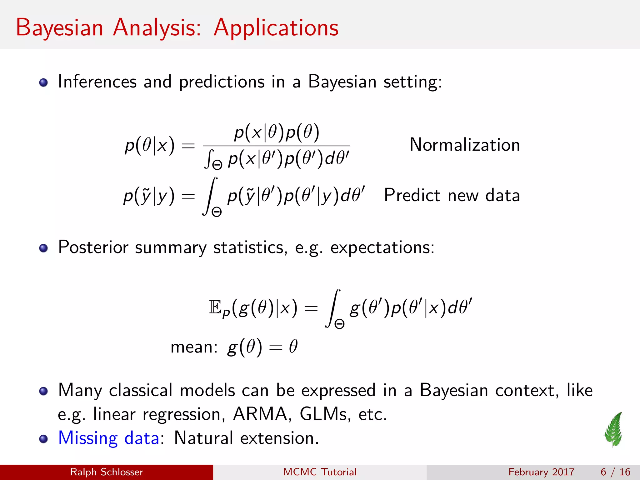
This document provides an introduction to Bayesian analysis and Metropolis-Hastings Markov chain Monte Carlo (MCMC). It explains the foundations of Bayesian analysis and how MCMC sampling methods like Metropolis-Hastings can be used to draw samples from posterior distributions that are intractable. The Metropolis-Hastings algorithm works by constructing a Markov chain with the target distribution as its stationary distribution. The document provides an example of using MCMC to perform linear regression in a Bayesian framework.

1. MCMC Tutorial
A short introduction to Bayesian Analysis and Metropolis-Hastings MCMC
Ralph Schlosser
https://github.com/bwv988
February 2017
Ralph Schlosser MCMC Tutorial February 2017 1 / 16

2. Overview
Bayesian Analysis
Monte Carlo Integration
Sampling Methods
Markov Chain Monte Carlo
Metropolis-Hastings Algorithm
Example: Linear Regression and M-H MCMC
Outlook
Ralph Schlosser MCMC Tutorial February 2017 2 / 16

3. Bayesian Analysis: Introduction
Foundation for MCMC: Bayesian
Analysis.
Frequentist – Likelihood model: p(x|θ)
How likely are the data x, given the
fixed parameters θ.
In general we want to estimate θ, e.g.
through MLE.
Bayesian – Bayesian model: p(θ|x).
Fundamental difference: In Bayesian
analysis, both parameter model and data
are treated as random variables.
Thomas Bayes (1707-1761)
Ralph Schlosser MCMC Tutorial February 2017 3 / 16

4. Bayesian Analysis: Terminology
From joint probability distribution to posterior distribution via data
likelihood and prior beliefs:
p(x, θ) = p(x|θ)p(θ)
p(θ|x) =
p(x, θ)
p(x)
=
p(x|θ)p(θ)
p(x)
Normalizing term p(x) difficult to get, but often not needed:
p(θ|x) ∝ p(x|θ)p(θ)
Posterior ∝ likelihood × prior
Ralph Schlosser MCMC Tutorial February 2017 4 / 16

5. Bayesian Analysis: Pros and Cons
Pro: Common-sense interpretability of results, e.g. Credible Intervals
vs. classical Confidence Intervals.
Pro: Update model parameters as new data becomes available.
Pro: Create hierarchical models through chaining:
p(φ, θ|x) = p(x|φ, θ)p(θ|φ)p(φ)
Hyperprior: p(θ|φ)p(φ)
Yesterdays posterior is tomorrow’s prior
Con: Must have a joint model for parameters, data, and prior.
What if we have absolutely no prior information?
Con: Choice of prior considered to be subjective.
Con: Subjectiveness makes comparison difficult.
Ralph Schlosser MCMC Tutorial February 2017 5 / 16

6. Bayesian Analysis: Applications
Inferences and predictions in a Bayesian setting:
p(θ|x) =
p(x|θ)p(θ)
Θ p(x|θ )p(θ )dθ
Normalization
p(˜y|y) =
Θ
p(˜y|θ )p(θ |y)dθ Predict new data
Posterior summary statistics, e.g. expectations:
Ep(g(θ)|x) =
Θ
g(θ )p(θ |x)dθ
mean: g(θ) = θ
Many classical models can be expressed in a Bayesian context, like
e.g. linear regression, ARMA, GLMs, etc.
Missing data: Natural extension.
Ralph Schlosser MCMC Tutorial February 2017 6 / 16

7. Monte Carlo Integration: Introduction
Applied Bayesian analysis asks to integrate over (often analytically
intractable) posterior densities.
Solution: Monte Carlo Integration
Suppose we wish to evaluate Ep(g(θ)|x) = Θ g(θ )p(θ |x)dθ
Given a set of N i.i.d. samples θ1, θ2, ..., θN from the density p:
Ep(g(θ|x)) ≈
1
N
N
i=1
g(θi )
But: Need to be able to draw random samples from p!
Ralph Schlosser MCMC Tutorial February 2017 7 / 16

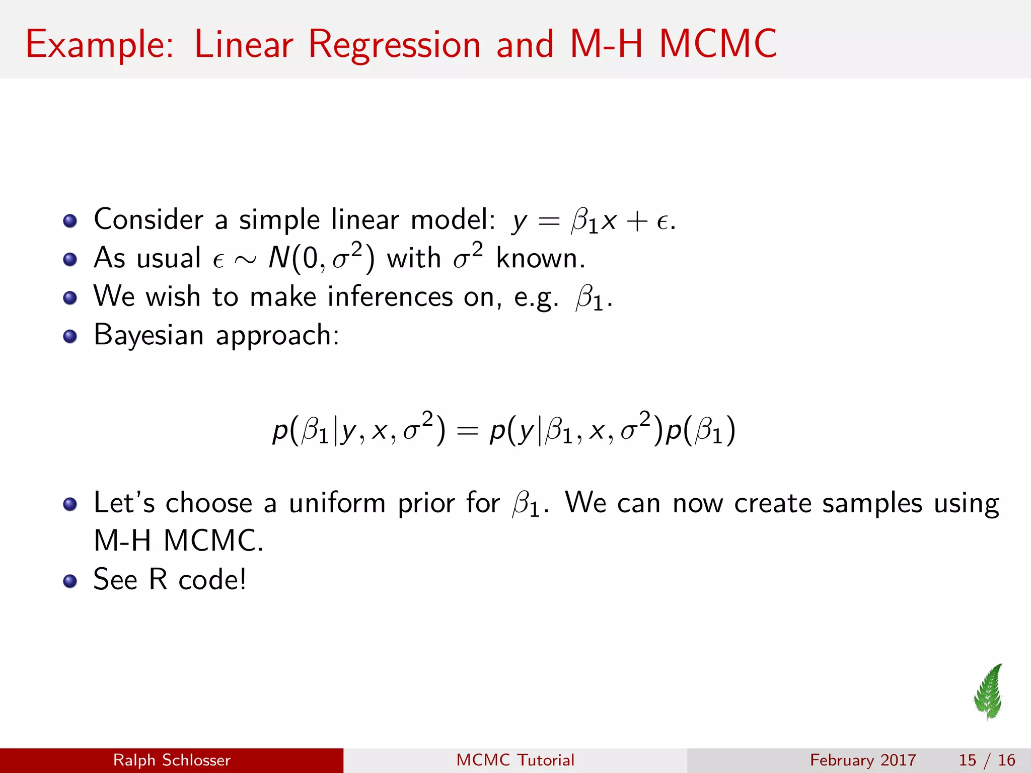
8. Monte Carlo Integration: Example
Simulate N = 10000 draws from a univariate standard normal, i.e.
X ∼ N(0, 1). Let p(x) be the normal density. Then:
P(X ≤ 0.5) =
0.5
−∞
p(x)dx
set.seed(123)
data <- rnorm(n = 10000)
prob.in <- data <= 0.5
sum(prob.in) / 10000
## [1] 0.694
pnorm(0.5)
## [1] 0.6914625
Ralph Schlosser MCMC Tutorial February 2017 8 / 16

9. Sampling Methods
Sampling from the posterior distribution is really important.
Classical sampling methods:
Inversion sampling
Importance sampling
Rejection sampling
Drawbacks:
Closed-form expression rarely accessible (Method of Inversion).
Doesn’t generalize well for highly-dimensional problems.
Metropolis-Hastings MCMC has largely superseded the above.
Ralph Schlosser MCMC Tutorial February 2017 9 / 16

10. Markov Chain Monte Carlo (MCMC)
Unlike pure Monte Carlo, in MCMC we create dependent samples.
Consider the target distribution p(θ|x) which is only known up to
proportionality.
Construct a Markov Chain in the state space of θ ∈ Θ with stationary
distribution p(θ|x).
Markov property – New state of chain depends only on previous state
(K: transitional kernel d.f.).
θt+1 = K(θ|θt)
With realizations {θt : t = 0, 1, ...} from the chain:
θt → p(θ|x)
1
N
N
t=1
g(θt) → Ep(g(θ|x)) a.s.
Ralph Schlosser MCMC Tutorial February 2017 10 / 16

11. Metropolis-Hastings MCMC: Intro & some history
An implementation of MCMC.
Originally developed by researchers Nicholas Metropolis, Stanislaw
Ulam, and co. at Los Alamos National Laboratories in the 1950’s.
Generalized through work done by Hastings in the 1970’s.
Popularized by a 1990 research paper from Gelfand & Smith:
http://wwwf.imperial.ac.uk/~das01/MyWeb/SCBI/Papers/
GelfandSmith.pdf
M-H MCMC really helped turning Bayesian analysis into practically
useful tool.
Ralph Schlosser MCMC Tutorial February 2017 11 / 16

12. Metropolis-Hastings MCMC: Terminology
M-H has two main ingredients.
A proposal distribution.
Dependent on the current chain state θt, generate a candidate for the
new state φ.
Written as q(θt, φ).
Can be chosen arbitrarily, but there are caveats (efficiency).
An acceptance probability.
Accept with probability α the move from the current state θt to state φ.
Written as α(θt, φ).
Main idea behind M-H: With every step, we want to get closer to the
target density (e.g. posterior density).
Ralph Schlosser MCMC Tutorial February 2017 12 / 16

13. Metropolis-Hastings MCMC: Intuition
Let’s call our target distribution (from which we want to sample) π.
At the core of the M-H algorithm we have the calculation of α(θt, φ):
α(θt, φ) = min 1,
π(φ)q(φ, θt)
π(θt)q(θt, φ)
Often q is symmetric, in which case it cancels out.
If π(φ)
π(θt ) > 1 → target density at the proposed new value is higher than
at current value.
In this case, we will accept the move from θt to φ with probability 1.
M-H really loves upward moves :)
Main point: Working with ratios of π, so only need π up to
proportionality!
Ralph Schlosser MCMC Tutorial February 2017 13 / 16

14. Metropolis-Hastings MCMC: Algorithm
1 Initialize θ0, number of iterations.
2 Given the current state θt, generate new state φ from the proposal
distribution q(θt, φ).
3 Calculate acceptance probability α(θt, φ).
4 With probability α(θt, φ), set θt+1 = φ, else set θt+1 = θt.
5 Iterate
6 Result: Realizations of dependent samples {θ1, θ2, ...} from the target
distribution π(θ).
Using these dependent realizations & due to the Monte Carlo approach, we
can now look at making inferences and predictions.
Ralph Schlosser MCMC Tutorial February 2017 14 / 16

15. Example: Linear Regression and M-H MCMC
Consider a simple linear model: y = β1x + .
As usual ∼ N(0, σ2) with σ2 known.
We wish to make inferences on, e.g. β1.
Bayesian approach:
p(β1|y, x, σ2
) = p(y|β1, x, σ2
)p(β1)
Let’s choose a uniform prior for β1. We can now create samples using
M-H MCMC.
See R code!
Ralph Schlosser MCMC Tutorial February 2017 15 / 16

16. Outlook
Many more interesting things could be mentioned, e.g. burn-in, choice
of q, Gibbs-sampling etc.
M-H and Monte Carlo in deep learning: http:
//www.deeplearningbook.org/contents/monte_carlo.html
Bayesian Deep Learning is a thing (apparently, don’t know anything
about it!)
Went way over my head, but looks cool – Finding the Higgs boson,
featuring Monte Carlo & Bayes: http://hea-www.harvard.edu/
AstroStat/Stat310_1314/dvd_20140121.pdf
Along the same lines, the amazing NIPS 2016 keynote: https:
//nips.cc/Conferences/2016/Schedule?showEvent=6195
M-H in Latent Dirichlet Allocation:
http://mlg.eng.cam.ac.uk/teaching/4f13/1112/lect10.pdf
Ralph Schlosser MCMC Tutorial February 2017 16 / 16