Approximative Bayesian Computation Methods

Approximative Bayesian Computation (ABC) Methods

Approximative Bayesian Computation
(ABC) Methods

Christian P. Robert

Universit´ Paris Dauphine and CREST-INSEE
e
http://www.ceremade.dauphine.fr/~xian

Joint works with M. Beaumont, J.-M. Cornuet, A. Grelaud,
J.-M. Marin, F. Rodolphe, & J.-F. Tally
Athens, September 14, 2009


Outline

1 Introduction

2 Population Monte Carlo

3 ABC

4 ABC-PMC

5 ABC for model choice in GRFs

Introduction

General purpose

Given a density π known up to a normalizing constant, and an
integrable function h, compute

h(x)˜ (x)µ(dx)
π
Π(h) = h(x)π(x)µ(dx) =
π (x)µ(dx)
˜

when h(x)˜ (x)µ(dx) is intractable.
π

Introduction
Monte Carlo basics

Monte Carlo basics
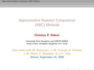
Generate an iid sample x1 , . . . , xN from π and estimate Π(h) by
N
ˆN
ΠM C (h) = N −1 h(xi ).
i=1

ˆN as
LLN: ΠM C (h) −→ Π(h)
If Π(h2 ) = h2 (x)π(x)µ(dx) < ∞,
√ L
CLT: ˆN
N ΠM C (h) − Π(h) N 0, Π [h − Π(h)]2 .

Introduction
Monte Carlo basics

Monte Carlo basics
Generate an iid sample x1 , . . . , xN from π and estimate Π(h) by
N
ˆN
ΠM C (h) = N −1 h(xi ).
i=1

ˆN as
LLN: ΠM C (h) −→ Π(h)
If Π(h2 ) = h2 (x)π(x)µ(dx) < ∞,
√ L
CLT: ˆN
N ΠM C (h) − Π(h) N 0, Π [h − Π(h)]2 .

Caveat
Often impossible or ineﬃcient to simulate directly from Π

Introduction
Importance Sampling

Importance Sampling

For Q proposal distribution such that Q(dx) = q(x)µ(dx),
alternative representation

Π(h) = h(x){π/q}(x)q(x)µ(dx).

Introduction
Importance Sampling

Importance Sampling

For Q proposal distribution such that Q(dx) = q(x)µ(dx),
alternative representation

Π(h) = h(x){π/q}(x)q(x)µ(dx).

Principle
Generate an iid sample x1 , . . . , xN ∼ Q and estimate Π(h) by
N
ˆ IS
ΠQ,N (h) = N −1 h(xi ){π/q}(xi ).
i=1

Introduction
Importance Sampling

Then
ˆ as
LLN: ΠIS (h) −→ Π(h)
Q,N and if Q((hπ/q)2 ) < ∞,
√ L
CLT: ˆ Q,N
N (ΠIS (h) − Π(h)) N 0, Q{(hπ/q − Π(h))2 } .

Introduction
Importance Sampling

Then
ˆ as
LLN: ΠIS (h) −→ Π(h)
Q,N and if Q((hπ/q)2 ) < ∞,
√ L
CLT: ˆ Q,N
N (ΠIS (h) − Π(h)) N 0, Q{(hπ/q − Π(h))2 } .

Caveat
ˆ Q,N
If normalizing constant unknown, impossible to use ΠIS

Generic problem in Bayesian Statistics: π(θ|x) ∝ f (x|θ)π(θ).

Introduction
Importance Sampling

Self-Normalised Importance Sampling

Self normalized version
N −1 N
ˆ Q,N
ΠSN IS (h) = {π/q}(xi ) h(xi ){π/q}(xi ).
i=1 i=1

Introduction
Importance Sampling


N −1 N
ˆ Q,N
i=1 i=1

ˆ as
LLN : ΠSN IS (h) −→ Π(h)
Q,N

and if Π((1 + h2 )(π/q)) < ∞,
√ L
CLT : ˆ Q,N
N (ΠSN IS (h) − Π(h)) N 0, π {(π/q)(h − Π(h)}2 ) .

Introduction
Importance Sampling


N −1 N
ˆ Q,N
i=1 i=1

ˆ as
LLN : ΠSN IS (h) −→ Π(h)
Q,N

and if Π((1 + h2 )(π/q)) < ∞,
√ L
CLT : ˆ Q,N
N (ΠSN IS (h) − Π(h)) N 0, π {(π/q)(h − Π(h)}2 ) .

c The quality of the SNIS approximation depends on the
choice of Q

Introduction
Importance Sampling

Iterated importance sampling

Introduction of an algorithmic temporal dimension :
(t) (t−1)
xi ∼ qt (x|xi ) i = 1, . . . , n, t = 1, . . .

and
n
ˆ 1 (t) (t)
It = ̺i h(xi )
n
i=1

is still unbiased for
(t)
(t) πt (xi )
̺i = (t) (t−1)
, i = 1, . . . , n
qt (xi |xi )

Population Monte Carlo

PMC: Population Monte Carlo Algorithm
At time t = 0
iid
Generate (xi,0 )1≤i≤N ∼ Q0
Set ωi,0 = {π/q0 }(xi,0 )
iid
Generate (Ji,0 )1≤i≤N ∼ M(1, (¯ i,0 )1≤i≤N )
ω
Set xi,0 = xJi ,0
˜


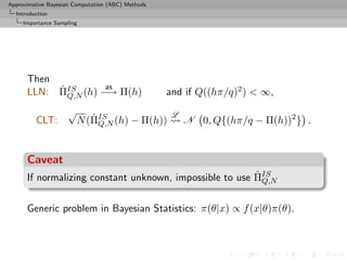
PMC: Population Monte Carlo Algorithm
At time t = 0
iid
Generate (xi,0 )1≤i≤N ∼ Q0
Set ωi,0 = {π/q0 }(xi,0 )
iid
Generate (Ji,0 )1≤i≤N ∼ M(1, (¯ i,0 )1≤i≤N )
ω
Set xi,0 = xJi ,0
˜
At time t (t = 1, . . . , T ),
ind
Generate xi,t ∼ Qi,t (˜i,t−1 , ·)
x
Set ωi,t = {π(xi,t )/qi,t (˜i,t−1 , xi,t )}
x
iid
Generate (Ji,t )1≤i≤N ∼ M(1, (¯ i,t )1≤i≤N )
ω
Set xi,t = xJi,t ,t .
˜

[Capp´, Douc, Guillin, Marin, & CPR, 2009, Stat.& Comput.]
e


Notes on PMC

After T iterations of PMC, PMC estimator of Π(h) given by
T N
¯ N,T 1
ΠP M C (h) = ωi,t h(xi,t ).
¯
T
t=1 i=1


Notes on PMC

After T iterations of PMC, PMC estimator of Π(h) given by
T N
¯ N,T 1
ΠP M C (h) = ωi,t h(xi,t ).
¯
T
t=1 i=1

1 ωi,t means normalising over whole sequence of simulations
¯
2 Qi,t ’s chosen arbitrarily under support constraint
3 Qi,t ’s may depend on whole sequence of simulations


Improving quality
The eﬃciency of the SNIS approximation depends on the choice of
Q, ranging from optimal

q(x) ∝ |h(x) − Π(h)|π(x)

to useless
ˆ Q,N
var ΠSN IS (h) = +∞


Improving quality
The eﬃciency of the SNIS approximation depends on the choice of
Q, ranging from optimal

q(x) ∝ |h(x) − Π(h)|π(x)

to useless
ˆ Q,N
var ΠSN IS (h) = +∞

Example (PMC=adaptive importance sampling)
Population Monte Carlo is producing a sequence of proposals Qt
aiming at improving eﬃciency

Kull(π, qt ) ≤ Kull(π, qt−1 ) or ˆ Q ,∞ ˆ Q ,∞
var ΠSN IS (h) ≤ var ΠSN IS (h)
t t−1

[Capp´, Douc, Guillin, Marin, Robert, 04, 07a, 07b, 08]
e

AMIS

Multiple Importance Sampling

Reycling: given several proposals Q1 , . . . , QT , for 1 ≤ t ≤ T
generate an iid sample

xt , . . . , xt ∼ Qt
1 N

and estimate Π(h) by
T N
ˆ Q,N
ΠM IS (h) = T −1 N −1
h(xt )ωi
i
t

t=1 i=1

where
t π(xt )
i
ωi = correct...
qt (xt )
i

AMIS

Multiple Importance Sampling

Reycling: given several proposals Q1 , . . . , QT , for 1 ≤ t ≤ T
generate an iid sample

xt , . . . , xt ∼ Qt
1 N

and estimate Π(h) by
T N
ˆ Q,N
ΠM IS (h) = T −1 N −1
h(xt )ωi
i
t

t=1 i=1

where
t π(xt )
i
ωi = T
still correct!
T −1 t
ℓ=1 qℓ (xi )

AMIS

Mixture representation

Deterministic mixture correction of the weights proposed by Owen
and Zhou (JASA, 2000)
The corresponding estimator is still unbiased [if not
self-normalised]
All particles are on the same weighting scale rather than their
own
Large variance proposals Qt do not take over
Variance reduction thanks to weight stabilization & recycling
[K.o.] removes the randomness in the component choice
[=Rao-Blackwellisation]

AMIS

Global adaptation

Global Adaptation
At iteration t = 1, · · · , T ,

1 µ ˆ
For 1 ≤ i ≤ N1 , generate xt ∼ T3 (ˆt−1 , Σt−1 )
i

2 Calculate the mixture importance weight of particle xt
i

ωi = π xt
t
i
t
δi

where
t−1
t
δi = i ˆ
ˆ
qT (3) xt ; µl , Σl
l=0

AMIS

Backward reweighting
3 If t ≥ 2, actualize the weights of all past particles, xl
i
1≤l ≤t−1
ωi = π xt δi
l
i
l

where
l l l
ˆ ˆ
δi = δi + qT (3) xi ; µt−1 , Σt−1

4 ˆ ˆ
Compute IS estimates of target mean and variance µt and Σt ,
where
t N1 t N1
µt
ˆj = ωi (xj )l
l
i
l
ωi . . .
l=1 i=1 l=1 i=1

AMIS

A toy example

10
0
−10
−20
−30

−40 −20 0 20 40

Banana shape benchmark: marginal distribution of (x1 , x2 ) for the
2
parameters σ1 = 100 and b = 0.03. Contours represent 60% (red),
90% (black) and 99.9% (blue) conﬁdence regions in the marginal
space.

AMIS

A toy example

p=5 p=10 p=20
1e+05

20000 40000 60000 80000

60000
8e+04
6e+04

20000
4e+04

0
Banana shape example: boxplots of 10 replicate ESSs for the AMIS
scheme (left) and the NOT-AMIS scheme (right) for p = 5, 10, 20.

Convergence of the estimator

Convergence of the AMIS estimator

Diﬃculty in establishing the convergence because of the backward
structure: the weight of xt at stage T depends on future as well as
i
past xℓ ’...
j
Regular Population Monte Carlo argument does not work for T
asymptotics...


Convergence of the AMIS estimator

Diﬃculty in establishing the convergence because of the backward
structure: the weight of xt at stage T depends on future as well as
i
past xℓ ’...
j
Regular Population Monte Carlo argument does not work for T
asymptotics...
[ c Amiss estimator?!]


A modiﬁed version of the algorithm

Only consider AMIS with p = 1, N = 1 and h(x) = x.

Set the variances of the t distributions to be equal to 1 after
rescaling, i.e. no learning process on the covariance matrix


Algorithmic setup

Our simpliﬁed algorithm then runs as follows:

π(x0 )x0
x0 ∼ q0 (·) , x1 ∼ T3 (u1 (x0 ), 1) where u1 (x0 ) = = µ0 ,
ˆ
q0 (x0 )

x2 ∼ T3 (u2 (x0:1 ), 1) where u2 (x0:1 ) =

π(x0 )x0 π(x1 )x1
+ = µ1 ,
ˆ
q0 (x0 ) + t3 (x0 ; u1 (x0 ), 1) q0 (x1 ) + t3 (x1 ; u1 (x0 ), 1)


Algorithmic setup (2)

xt ∼ T3 (ut (x0:t−1 ), 1)
t−1
π(xk )xk
where ut (x0:t−1 ) = t−1 ,...
q (x ) +
k=0 0 k i=1 t3 (xk ; ui (x0:i−1 ), 1)


Stumbling block

Establishing that
T
T π(xk )xk L2
µ =
ˆ T
−→ µ = xπ(x)dx .
k=0
q0 (xk ) + i=1 t3 (xk ; ui (x0:i−1 ), 1)
T →∞

proves to be surprisingly diﬃcult (note that E(ˆT ) = µ)
µ
Impossible to use PMC convergence theorems on triangular
arrays of random variables.

An unbiased estimator

Unbiased version of the estimator

Modiﬁed version of previous algorithm with two sequences:

x0 ∼ q0 (·) and x0 ∼ q0 (·) ,
˜

x1 ∼ T3 (u1 (˜0 ), 1) and x1 ∼ T3 (u1 (˜0 ), 1)
x ˜ x
π(˜0 )˜0
x x
where u1 (˜0 ) =
x = µ0 ,
ˆ
q0 (˜0 )
x

x2 ∼ T3 (u2 (˜0:1 ), 1) and x2 ∼ T3 (u2 (˜0:1 ), 1) where u2 (˜0:1 ) =
x ˜ x x
π(˜0 )˜0
x x π(˜1 )˜1
x x 1
+ =µ ,
ˆ
q0 (˜0 ) + t3 (˜0 ; u1 (˜0 ), 1) q0 (˜1 ) + t3 (˜1 ; u1 (˜0 ), 1)
x x x x x x


Unbiased version of the estimator (2)

xt ∼ T3 (ut (x0:t−1 ), 1) and xt ∼ T3 (ut (˜0:t−1 ), 1)
˜ x
t−1
π(˜k )˜k
x x
where ut (˜0:t−1 ) =
x t−1 ,...
k=0
q0 (˜k ) +
x i=1 t3 (˜k ; ui (˜0:i−1 ), 1)
x x

Let
T
π(xk )xk
µT =
ˆU T
.
q (x ) +
k=0 0 k i=1 t3 (xk ; ui (˜0:i−1 ), 1)
x


My questions

Clearly, we have
E(ˆT ) = µ
µU
and under mild conditions we should have
L
µT −→ µ
ˆU 2
T →∞


My questions

Clearly, we have
E(ˆT ) = µ
µU
and under mild conditions we should have
L
µT −→ µ
ˆU 2
T →∞

Except for the compact case, i.e. when supp(π) is compact, this
also proves impossible to establish...
µT
The only indication we have is that var(ˆU ) is decreasing at each
iteration

ABC

The ABC method

Bayesian setting: target is π(θ)f (x|θ)

ABC

The ABC method

When likelihood f (x|θ) not in closed form, likelihood-free rejection
technique:

ABC

The ABC method

When likelihood f (x|θ) not in closed form, likelihood-free rejection
technique:
ABC algorithm
For an observation y ∼ f (y|θ), under the prior π(θ), keep jointly
simulating
θ′ ∼ π(θ) , x ∼ f (x|θ′ ) ,
until the auxiliary variable x is equal to the observed value, x = y.

[Pritchard et al., 1999]

ABC

A as approximative

When y is a continuous random variable, equality x = y is replaced
with a tolerance condition,

̺(x, y) ≤ ǫ

where ̺ is a distance between summary statistics

ABC

A as approximative

When y is a continuous random variable, equality x = y is replaced
with a tolerance condition,

̺(x, y) ≤ ǫ

where ̺ is a distance between summary statistics
Output distributed from

π(θ) Pθ {̺(x, y) < ǫ} ∝ π(θ|̺(x, y) < ǫ)

ABC

ABC improvements

Simulating from the prior is often poor in eﬃciency

ABC

ABC improvements

Either modify the proposal distribution on θ to increase the density
of x’s within the vicinity of y...
[Marjoram et al, 2003; Bortot et al., 2007, Sisson et al., 2007]

ABC

ABC improvements


...or by viewing the problem as a conditional density estimation
and by developing techniques to allow for larger ǫ
[Beaumont et al., 2002]

ABC

ABC improvements


...or by viewing the problem as a conditional density estimation
and by developing techniques to allow for larger ǫ
[Beaumont et al., 2002]

...or even by including ǫ in the inferential framework [ABCµ ]
[Ratmann et al., 2009]

ABC

ABC-MCMC

Markov chain (θ(t) ) created via the transition function

θ′ ∼ K(θ′ |θ(t) ) if x ∼ f (x|θ′ ) is such that x = y


(t+1) π(θ′ )K(θ(t) |θ′ )
θ = and u ∼ U(0, 1) ≤ π(θ(t) )K(θ′ |θ(t) ) ,

 (t)
θ otherwise,

ABC

ABC-MCMC

Markov chain (θ(t) ) created via the transition function

θ′ ∼ K(θ′ |θ(t) ) if x ∼ f (x|θ′ ) is such that x = y


(t+1) π(θ′ )K(θ(t) |θ′ )
θ = and u ∼ U(0, 1) ≤ π(θ(t) )K(θ′ |θ(t) ) ,

 (t)
θ otherwise,

has the posterior π(θ|y) as stationary distribution
[Marjoram et al, 2003]

ABC

ABCµ

[Ratmann, Andrieu, Wiuf and Richardson, 2009, PNAS]

Use of a joint density

f (θ, ǫ|x0 ) ∝ ξ(ǫ|x0 , θ) × πθ (θ) × πǫ (ǫ)

where x0 is the data, and ξ(ǫ|x0 , θ) is the prior predictive density
of ρ(S(x), S(x0 )) given θ and x0 when x ∼ f (x|θ)
Replacement of ξ(ǫ|x0 , θ) with a non-parametric kernel
approximation.

ABC

Questions about ABCµ

For each model under comparison, marginal posterior on ǫ used to
assess the ﬁt of the model (HPD includes 0 or not).

ABC

Questions about ABCµ

For each model under comparison, marginal posterior on ǫ used to
assess the ﬁt of the model (HPD includes 0 or not).
Is the data informative about ǫ? [Identiﬁability]
How is the prior π(ǫ) impacting the comparison?
How is using both ξ(ǫ|x0 , θ) and πǫ (ǫ) compatible with a
standard probability model?
Where is there a penalisation for complexity in the model
comparison?

ABC

ABC-PRC

Another sequential version producing a sequence of Markov
(t) (t)
transition kernels Kt and of samples (θ1 , . . . , θN ) (1 ≤ t ≤ T )

ABC

ABC-PRC

Another sequential version producing a sequence of Markov
(t) (t)
transition kernels Kt and of samples (θ1 , . . . , θN ) (1 ≤ t ≤ T )

ABC-PRC Algorithm
(t−1)
1 Pick a θ⋆ is selected at random among the previous θi ’s
(t−1)
with probabilities ωi (1 ≤ i ≤ N ).
2 Generate
(t) (t)
θi ∼ Kt (θ|θ⋆ ) , x ∼ f (x|θi ) ,
3 Check that ̺(x, y) < ǫ, otherwise start again.

[Sisson et al., 2007]

ABC

ABC-PRC weight

(t)
Probability ωi computed as
(t) (t) (t) (t)
ωi ∝ π(θi )Lt−1 (θ⋆ |θi ){π(θ⋆ )Kt (θi |θ⋆ )}−1 ,

where Lt−1 is an arbitrary transition kernel.

ABC

ABC-PRC weight

(t)
(t) (t) (t) (t)

In case
Lt−1 (θ′ |θ) = Kt (θ|θ′ ) ,
all weights are equal under a uniform prior.

ABC

ABC-PRC weight

(t)
(t) (t) (t) (t)

In case
Lt−1 (θ′ |θ) = Kt (θ|θ′ ) ,
all weights are equal under a uniform prior.
Inspired from Del Moral et al. (2006), who use backward kernels
Lt−1 in SMC to achieve unbiasedness

ABC

ABC-PRC bias
Lack of unbiasedness of the method

ABC

A mixture example
0.8

0.8

0.8

0.8

0.8
0.4

0.4

0.4

0.4

0.4
0.0

0.0

0.0

0.0

0.0
−3 −1 1 2 3 −3 −1 1 2 3 −3 −1 1 2 3 −3 −1 1 2 3 −3 −1 1 2 3

θ θ θ θ θ
0.8

0.8

0.8

0.8

0.8
0.4

0.4

0.4

0.4

0.4
0.0

0.0

0.0

0.0

0.0
−3 −1 1 2 3 −3 −1 1 2 3 −3 −1 1 2 3 −3 −1 1 2 3 −3 −1 1 2 3

θ θ θ θ θ

Comparison of τ = 0.15 and τ = 1/0.15 in Kt

ABC-PMC

A PMC version
Use of the same kernel idea as ABC-PRC but with IS correction
Generate a sample at iteration t by
N
(t−1) (t−1)
πt (θ(t) ) ∝
ˆ ωj Kt (θ(t) |θj )
j=1

modulo acceptance of the associated xt , and use an importance
(t)
weight associated with an accepted simulation θi
(t) (t) (t)
ωi ∝ π(θi ) πt (θi ) .
ˆ

c Still likelihood free
[Beaumont et al., 2008, arXiv:0805.2256]

ABC-PMC

The ABC-PMC algorithm
Given a decreasing sequence of approximation levels ǫ1 ≥ . . . ≥ ǫT ,
1. At iteration t = 1,
For i = 1, ..., N
(1) (1)
Simulate θi ∼ π(θ) and x ∼ f (x|θi ) until ̺(x, y) < ǫ1
(1)
Set ωi = 1/N
(1)
Take τ 2 as twice the empirical variance of the θi ’s
2. At iteration 2 ≤ t ≤ T ,
For i = 1, ..., N , repeat
⋆ (t−1) (t−1)
Pick θi from the θj ’s with probabilities ωj
(t)
⋆ ⋆ 2 (t)
generate θi |θi ∼ N (θi , σt ) and x ∼ f (x|θi )
until ̺(x, y) < ǫt
(t) (t) N (t−1) (t) (t−1)
Set ωi ∝ π(θi )/ j=1 ωj ϕ σt
−1
θi − θj )
2 (t)
Take τt+1 as twice the weighted empirical variance of the θi ’s

ABC-PMC

ABC-SMC
[Del Moral, Doucet & Jasra, 2009]

True derivation of an SMC-ABC algorithm
Use of a kernel Kn associated with target πǫn and derivation of the
backward kernel
πǫn (z ′ )Kn (z ′ , z)
Ln−1 (z, z ′ ) =
πn (z)

Update of the weights
M m
m=1 Aǫ⋉ (xin
win ∝i(n−1) M m
m=1 Aǫ⋉− (xi(n−1)

when xm ∼ K(xi(n−1) , ·)
in

ABC-PMC

A mixture example (0)

Toy model of Sisson et al. (2007): if

θ ∼ U(−10, 10) , x|θ ∼ 0.5 N (θ, 1) + 0.5 N (θ, 1/100) ,

then the posterior distribution associated with y = 0 is the normal
mixture
θ|y = 0 ∼ 0.5 N (0, 1) + 0.5 N (0, 1/100)
restricted to [−10, 10].
Furthermore, true target available as

π(θ||x| < ǫ) ∝ Φ(ǫ−θ)−Φ(−ǫ−θ)+Φ(10(ǫ−θ))−Φ(−10(ǫ+θ)) .

ABC-PMC

A mixture example (2)
Recovery of the target, whether using a ﬁxed standard deviation of
τ = 0.15 or τ = 1/0.15, or a sequence of adaptive τt ’s.

ABC for model choice in GRFs

ABC for model choice

1 Introduction

2 Population Monte Carlo

3 ABC

4 ABC-PMC

5 ABC for model choice in GRFs
Gibbs random ﬁelds
Model choice via ABC
Illustrations



Gibbs distribution
The rv y = (y1 , . . . , yn ) is a Gibbs random ﬁeld associated with
the graph G if

1
f (y) = exp − Vc (yc ) ,
Z
c∈C

where Z is the normalising constant, C is the set of cliques of G
and Vc is any function also called potential
U (y) = c∈C Vc (yc ) is the energy function



Gibbs distribution
The rv y = (y1 , . . . , yn ) is a Gibbs random ﬁeld associated with
the graph G if

1
f (y) = exp − Vc (yc ) ,
Z
c∈C

where Z is the normalising constant, C is the set of cliques of G
and Vc is any function also called potential
U (y) = c∈C Vc (yc ) is the energy function

c Z is usually unavailable in closed form


Potts model
Potts model
Vc (y) is of the form

Vc (y) = θS(y) = θ δyl =yi
l∼i

where l∼i denotes a neighbourhood structure


Potts model
Potts model
Vc (y) is of the form

Vc (y) = θS(y) = θ δyl =yi
l∼i

where l∼i denotes a neighbourhood structure

In most realistic settings, summation

Zθ = exp{θT S(x)}
x∈X

involves too many terms to be manageable and numerical
approximations cannot always be trusted
[Cucala, Marin, CPR & Titterington, 2009]


Bayesian Model Choice

Comparing a model with potential S0 taking values in Rp0 versus a
model with potential S1 taking values in Rp1 can be done through
the Bayes factor corresponding to the priors π0 and π1 on each
parameter space
T
exp{θ0 S0 (x)}/Zθ0 ,0 π0 (dθ0 )
Bm0 /m1 (x) = T
exp{θ1 S1 (x)}/Zθ1 ,1 π1 (dθ1 )


Bayesian Model Choice

Comparing a model with potential S0 taking values in Rp0 versus a
model with potential S1 taking values in Rp1 can be done through
the Bayes factor corresponding to the priors π0 and π1 on each
parameter space
T
exp{θ0 S0 (x)}/Zθ0 ,0 π0 (dθ0 )
Bm0 /m1 (x) = T
exp{θ1 S1 (x)}/Zθ1 ,1 π1 (dθ1 )

Use of Jeﬀreys’ scale to select most appropriate model


Neighbourhood relations

Choice to be made between M neighbourhood relations
m
i ∼ i′ (0 ≤ m ≤ M − 1)

with
Sm (x) = I{xi =xi′ }
m
i∼i′

driven by the posterior probabilities of the models.


Model index

Formalisation via a model index M that appears as a new
parameter with prior distribution π(M = m) and
π(θ|M = m) = πm (θm )


Model index

Formalisation via a model index M that appears as a new
parameter with prior distribution π(M = m) and
π(θ|M = m) = πm (θm )
Computational target:

P(M = m|x) ∝ fm (x|θm )πm (θm ) dθm π(M = m) ,
Θm


Sufficient statistics
By definition, if S(x) sufficient statistic for the joint parameters
(M, θ0 , . . . , θM −1 ),
P(M = m|x) = P(M = m|S(x)) .


(M, θ0 , . . . , θM −1 ),
P(M = m|x) = P(M = m|S(x)) .
For each model m, own suﬃcient statistic Sm (·) and
S(·) = (S0 (·), . . . , SM −1 (·)) also suﬃcient.


(M, θ0 , . . . , θM −1 ),
P(M = m|x) = P(M = m|S(x)) .
For each model m, own sufficient statistic Sm (·) and
S(·) = (S0 (·), . . . , SM −1 (·)) also sufficient.
For Gibbs random fields,
1 2
x|M = m ∼ fm (x|θm ) = fm (x|S(x))fm (S(x)|θm )
1
= f 2 (S(x)|θm )
n(S(x)) m
where
n(S(x)) = ♯ {˜ ∈ X : S(˜ ) = S(x)}
x x
c S(x) is therefore also sufficient for the joint parameters
[Specific to Gibbs random fields!]


ABC model choice Algorithm

ABC-MC
Generate m∗ from the prior π(M = m).
∗
Generate θm∗ from the prior πm∗ (·).
∗
Generate x∗ from the model fm∗ (·|θm∗ ).
Compute the distance ρ(S(x0 ), S(x∗ )).
∗
Accept (θm∗ , m∗ ) if ρ(S(x0 ), S(x∗ )) < ǫ.

Note When ǫ = 0 the algorithm is exact


ABC approximation to the Bayes factor

Frequency ratio:
ˆ
P(M = m0 |x0 ) π(M = m1 )
BF m0 /m1 (x0 ) = ×
ˆ
P(M = m1 |x0 ) π(M = m0 )
♯{mi∗ = m0 } π(M = m1 )
= × ,
♯{mi∗ = m1 } π(M = m0 )


ABC approximation to the Bayes factor

Frequency ratio:
ˆ
P(M = m0 |x0 ) π(M = m1 )
BF m0 /m1 (x0 ) = ×
ˆ
P(M = m1 |x0 ) π(M = m0 )
♯{mi∗ = m0 } π(M = m1 )
= × ,
♯{mi∗ = m1 } π(M = m0 )

replaced with

1 + ♯{mi∗ = m0 } π(M = m1 )
BF m0 /m1 (x0 ) = ×
1 + ♯{mi∗ = m1 } π(M = m0 )

to avoid indeterminacy (also Bayes estimate).

Illustrations

Toy example

iid Bernoulli model versus two-state ﬁrst-order Markov chain, i.e.
n
f0 (x|θ0 ) = exp θ0 I{xi =1} {1 + exp(θ0 )}n ,
i=1

versus
n
1
f1 (x|θ1 ) = exp θ1 I{xi =xi−1 } {1 + exp(θ1 )}n−1 ,
2
i=2

with priors θ0 ∼ U(−5, 5) and θ1 ∼ U(0, 6) (inspired by “phase
transition” boundaries).

Illustrations

Toy example (2)

10
5

5
BF01

BF01

0
0
^

^

−10 −5
−5

−40 −20 0 10 −40 −20 0 10

BF01 BF01

(left) Comparison of the true BF m0 /m1 (x0 ) with BF m0 /m1 (x0 )
(in logs) over 2, 000 simulations and 4.106 proposals from the
prior. (right) Same when using tolerance ǫ corresponding to the
1% quantile on the distances.

Illustrations

Protein folding

Superposition of the native structure (grey) with the ST1
structure (red.), the ST2 structure (orange), the ST3 structure
(green), and the DT structure (blue).

Illustrations

Protein folding (2)

% seq . Id. TM-score FROST score
1i5nA (ST1) 32 0.86 75.3
1ls1A1 (ST2) 5 0.42 8.9
1jr8A (ST3) 4 0.24 8.9
1s7oA (DT) 10 0.08 7.8

Characteristics of dataset. % seq. Id.: percentage of identity with
the query sequence. TM-score.: similarity between predicted and
native structure (uncertainty between 0.17 and 0.4) FROST score:
quality of alignment of the query onto the candidate structure
(uncertainty between 7 and 9).

Illustrations

Protein folding (3)

NS/ST1 NS/ST2 NS/ST3 NS/DT
BF 1.34 1.22 2.42 2.76
P(M = NS|x0 ) 0.573 0.551 0.708 0.734

Estimates of the Bayes factors between model NS and models
ST1, ST2, ST3, and DT, and corresponding posterior
probabilities of model NS based on an ABC-MC algorithm using
1.2 106 simulations and a tolerance ǫ equal to the 1% quantile of
the distances.

Approximative Bayesian Computation Methods

Recommended

Recommended

More Related Content

What's hot

What's hot (19)

Viewers also liked

Viewers also liked (9)

Similar to Approximative Bayesian Computation Methods

Similar to Approximative Bayesian Computation Methods (20)

More from Christian Robert

More from Christian Robert (20)

Recently uploaded

Recently uploaded (20)

Approximative Bayesian Computation Methods