Download as PDF, PPTX


![Is there a calculus for distributed computing?
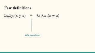
“The inevitability of the lambda-calculus arises
from the fact that the only way to observe a
functional computation is to watch which output
values it yields when presented with different
input values” [1]](https://image.slidesharecdn.com/understandingdistributedcalculiinhaskell-180304222304/85/Understanding-distributed-calculi-in-Haskell-97-320.jpg)
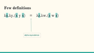
![Is there a calculus for distributed computing?
“Unfortunately, the world of concurrent
computation is not so orderly. Different notions of
what can be observed may be appropriate in
different circumstances, giving rise to different
definitions of when two concurrent systems have
‘the same behavior’ ” [1]](https://image.slidesharecdn.com/understandingdistributedcalculiinhaskell-180304222304/85/Understanding-distributed-calculi-in-Haskell-98-320.jpg)

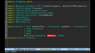
![CCS & CSP
CCS - Calculus of Communicating Systems [3]
CSP - Communicating Sequential Processes [4]](https://image.slidesharecdn.com/understandingdistributedcalculiinhaskell-180304222304/85/Understanding-distributed-calculi-in-Haskell-100-320.jpg)

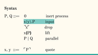
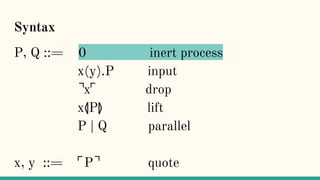
![What is π-calculus
“π -calculus is a model of computation for
concurrent systems.” [2]](https://image.slidesharecdn.com/understandingdistributedcalculiinhaskell-180304222304/85/Understanding-distributed-calculi-in-Haskell-102-320.jpg)
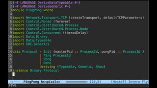
![What is π-calculus
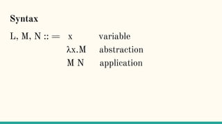
“In lambda-calculus everything is a function (...)
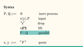
In the pi-calculus every expression denotes a
process - a free-standing computational activity,
running in parallel with other process.” [1]](https://image.slidesharecdn.com/understandingdistributedcalculiinhaskell-180304222304/85/Understanding-distributed-calculi-in-Haskell-103-320.jpg)
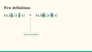
![What is π-calculus
“Two processes can interact by exchanging a
message on a channel” [1]](https://image.slidesharecdn.com/understandingdistributedcalculiinhaskell-180304222304/85/Understanding-distributed-calculi-in-Haskell-104-320.jpg)
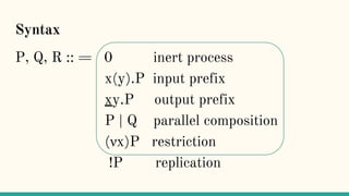
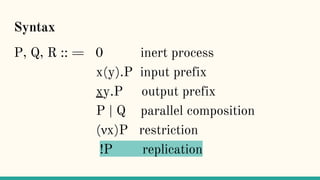
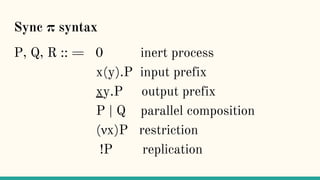
![What is π-calculus
“It lets you represent processes, parallel
composition of processes, synchronous
communication between processes through
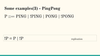
channels, creation of fresh channels, replication of
processes, and nondeterminism.” [2]](https://image.slidesharecdn.com/understandingdistributedcalculiinhaskell-180304222304/85/Understanding-distributed-calculi-in-Haskell-105-320.jpg)
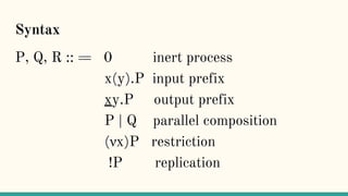


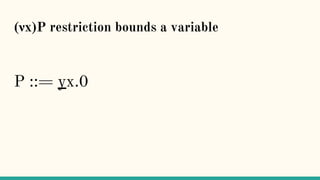
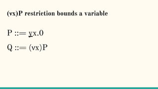
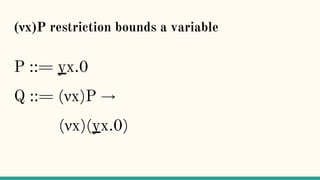
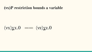


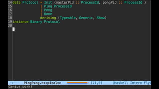
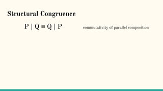
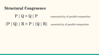
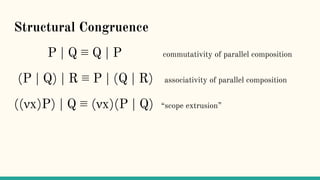
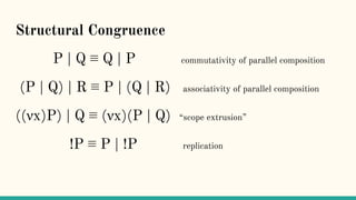
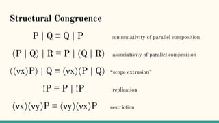
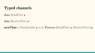
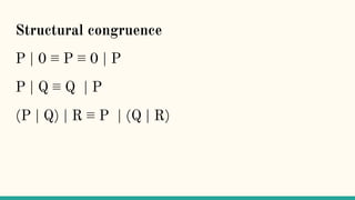
![Structural Congruence
“Two processes are structurally congruent, if they
are identical up to structure.” [5]](https://image.slidesharecdn.com/understandingdistributedcalculiinhaskell-180304222304/85/Understanding-distributed-calculi-in-Haskell-148-320.jpg)
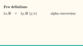
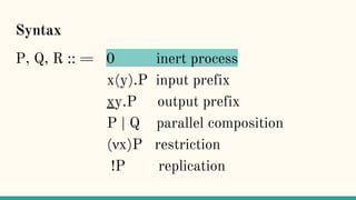
![Reduction rules ⟶
xy.P | x(z).Q → P | [y/z]Q communication](https://image.slidesharecdn.com/understandingdistributedcalculiinhaskell-180304222304/85/Understanding-distributed-calculi-in-Haskell-157-320.jpg)
![Reduction rules ⟶
xy.P | x(z).Q → P | [y/z]Q communication
P | R → if P → Q reduction under |](https://image.slidesharecdn.com/understandingdistributedcalculiinhaskell-180304222304/85/Understanding-distributed-calculi-in-Haskell-158-320.jpg)
![Reduction rules ⟶
xy.P | x(z).Q → P | [y/z]Q communication
P | R → Q | R if P → Q reduction under |](https://image.slidesharecdn.com/understandingdistributedcalculiinhaskell-180304222304/85/Understanding-distributed-calculi-in-Haskell-159-320.jpg)
![Reduction rules ⟶
xy.P | x(z).Q → P | [y/z]Q communication
P | R → Q | R if P → Q reduction under |
(νx)P → if P → Q reduction under ν](https://image.slidesharecdn.com/understandingdistributedcalculiinhaskell-180304222304/85/Understanding-distributed-calculi-in-Haskell-160-320.jpg)
![Reduction rules ⟶
xy.P | x(z).Q → P | [y/z]Q communication
P | R → Q | R if P → Q reduction under |
(νx)P → (νx)Q if P → Q reduction under ν](https://image.slidesharecdn.com/understandingdistributedcalculiinhaskell-180304222304/85/Understanding-distributed-calculi-in-Haskell-161-320.jpg)
![Reduction rules ⟶
xy.P | x(z).Q → P | [y/z]Q communication
P | R → Q | R if P → Q reduction under |
(νx)P → (νx)Q if P → Q reduction under ν
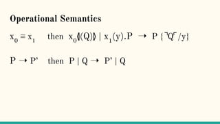
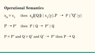
P → if P ≡ P’ Q’ ≡ Q structural congruence](https://image.slidesharecdn.com/understandingdistributedcalculiinhaskell-180304222304/85/Understanding-distributed-calculi-in-Haskell-162-320.jpg)
![Reduction rules ⟶
xy.P | x(z).Q → P | [y/z]Q communication
P | R → Q | R if P → Q reduction under |
(νx)P → (νx)Q if P → Q reduction under ν
P → if P ≡ P’ → Q’ ≡ Q structural congruence](https://image.slidesharecdn.com/understandingdistributedcalculiinhaskell-180304222304/85/Understanding-distributed-calculi-in-Haskell-163-320.jpg)
![Reduction rules ⟶
xy.P | x(z).Q → P | [y/z]Q communication
P | R → Q | R if P → Q reduction under |
(νx)P → (νx)Q if P → Q reduction under ν
P → Q if P ≡ P’ → Q’ ≡ Q structural congruence](https://image.slidesharecdn.com/understandingdistributedcalculiinhaskell-180304222304/85/Understanding-distributed-calculi-in-Haskell-164-320.jpg)
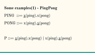
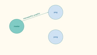
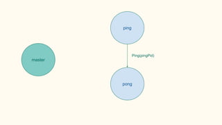
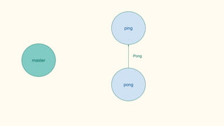
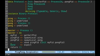
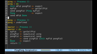
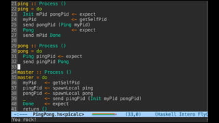
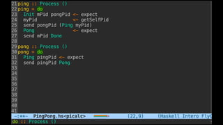
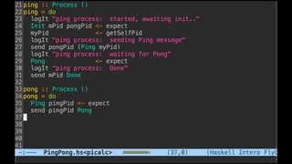
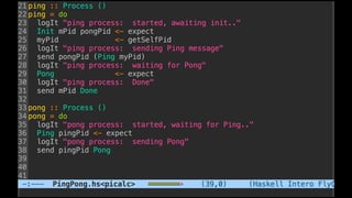
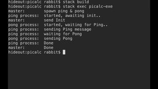
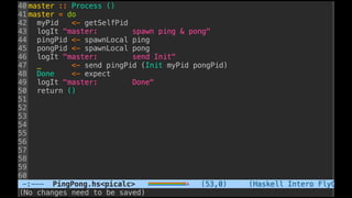
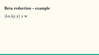
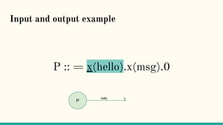
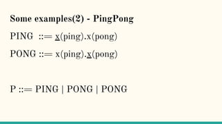
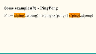
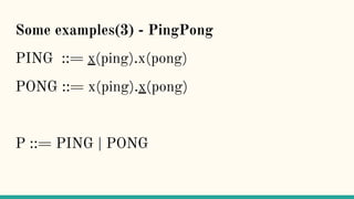
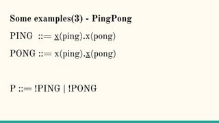
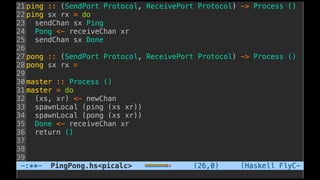
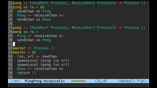
![Some examples(1) - PingPong
P ::= x(ping).x(pong) | x(ping).x(pong)
xy.P | x(z).Q → P | [y/z]Q communication](https://image.slidesharecdn.com/understandingdistributedcalculiinhaskell-180304222304/85/Understanding-distributed-calculi-in-Haskell-168-320.jpg)
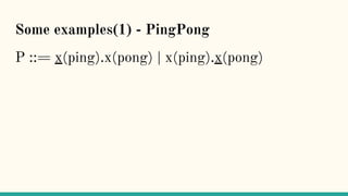
![Some examples(1) - PingPong
P ::= x(ping).x(pong) | x(ping).x(pong)
xy.P | x(z).Q → P | [y/z]Q communication](https://image.slidesharecdn.com/understandingdistributedcalculiinhaskell-180304222304/85/Understanding-distributed-calculi-in-Haskell-169-320.jpg)
![Some examples(1) - PingPong
P ::= x(ping).x(pong) | x(ping).x(pong)
xy.P | x(z).Q → P | [y/z]Q communication](https://image.slidesharecdn.com/understandingdistributedcalculiinhaskell-180304222304/85/Understanding-distributed-calculi-in-Haskell-170-320.jpg)
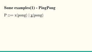
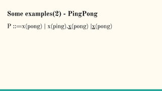
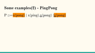
![Some examples(1) - PingPong
P ::= x(pong) | x(pong)
xy.P | x(z).Q → P | [y/z]Q communication](https://image.slidesharecdn.com/understandingdistributedcalculiinhaskell-180304222304/85/Understanding-distributed-calculi-in-Haskell-171-320.jpg)
![Some examples(1) - PingPong
P ::= x(pong) | x(pong)
xy.P | x(z).Q → P | [y/z]Q communication](https://image.slidesharecdn.com/understandingdistributedcalculiinhaskell-180304222304/85/Understanding-distributed-calculi-in-Haskell-173-320.jpg)
![Some examples(1) - PingPong
P ::= x(pong) | x(pong)
xy.P | x(z).Q → P | [y/z]Q communication](https://image.slidesharecdn.com/understandingdistributedcalculiinhaskell-180304222304/85/Understanding-distributed-calculi-in-Haskell-174-320.jpg)
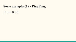
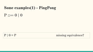
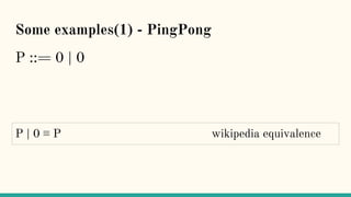
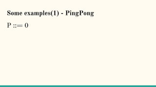
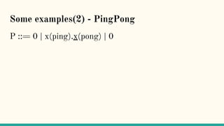
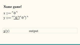
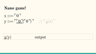
![Some examples(1) - PingPong
P ::= 0 | 0
xy.P | x(z).Q → P | [y/z]Q communication](https://image.slidesharecdn.com/understandingdistributedcalculiinhaskell-180304222304/85/Understanding-distributed-calculi-in-Haskell-175-320.jpg)

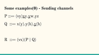
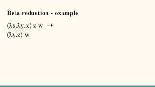
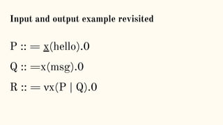
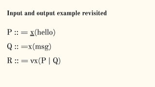
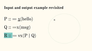
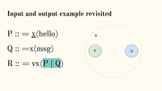
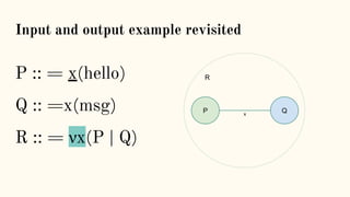
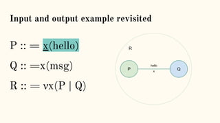
![Some examples(0) - Sending channels
P ::= (νy)xy.yw.yz
Q ::= x(y).y(h).y(h)
R ::= (νx)((νy)xy.yw.yz | x(y).y(h).y(h))
xy.P | x(z).Q → P | [y/z]Q communication](https://image.slidesharecdn.com/understandingdistributedcalculiinhaskell-180304222304/85/Understanding-distributed-calculi-in-Haskell-184-320.jpg)
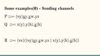
![Some examples(0) - Sending channels
P ::= (νy)xy.yw.yz
Q ::= x(y).y(h).y(h)
R ::= (νx)((νy)xy.yw.yz | x(y).y(h).y(h))
xy.P | x(z).Q → P | [y/z]Q communication](https://image.slidesharecdn.com/understandingdistributedcalculiinhaskell-180304222304/85/Understanding-distributed-calculi-in-Haskell-185-320.jpg)
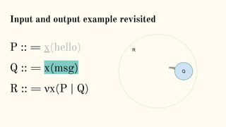
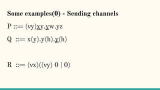
![Some examples(0) - Sending channels
P ::= (νy)xy.yw.yz
Q ::= x(y).y(h).y(h)
R ::= (νx)((νy)yw.yz | y(h).y(h))
xy.P | x(z).Q → P | [y/z]Q communication](https://image.slidesharecdn.com/understandingdistributedcalculiinhaskell-180304222304/85/Understanding-distributed-calculi-in-Haskell-186-320.jpg)
![Some examples(0) - Sending channels
P ::= (νy)xy.yw.yz
Q ::= x(y).y(h).y(h)
R ::= (νx)((νy)yw.yz | y(h).y(h))
xy.P | x(z).Q → P | [y/z]Q communication](https://image.slidesharecdn.com/understandingdistributedcalculiinhaskell-180304222304/85/Understanding-distributed-calculi-in-Haskell-187-320.jpg)
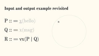
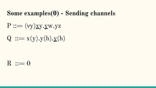
![Some examples(0) - Sending channels
P ::= (νy)xy.yw.yz
Q ::= x(y).y(h).y(h)
R ::= (νx)((νy)yz | y(h))
xy.P | x(z).Q → P | [y/z]Q communication](https://image.slidesharecdn.com/understandingdistributedcalculiinhaskell-180304222304/85/Understanding-distributed-calculi-in-Haskell-188-320.jpg)

![Two processes P and Q are bisimilar if ...
“Two processes P and Q are bisimilar if every
action of one can be matched by a corresponding
action of the other to reach bisimilar state” [1]](https://image.slidesharecdn.com/understandingdistributedcalculiinhaskell-180304222304/85/Understanding-distributed-calculi-in-Haskell-215-320.jpg)


![Implementation issue...
“This seems quite natural.(...).But there’s a big problem here.
ReceivePorts are not Serializable, which prevents us passing
the ReceivePort r1 to the spawned process. GHC will reject the
program with a type error.” [8]](https://image.slidesharecdn.com/understandingdistributedcalculiinhaskell-180304222304/85/Understanding-distributed-calculi-in-Haskell-225-320.jpg)
![Implementation issue...
“Why are ReceivePorts not Serializable? If you think about it a
bit, this makes a lot of sense. If a process were allowed to send
a ReceivePort somewhere else, the implementation would have
to deal with two things: routing messages to the correct desti‐
nation when a ReceivePort has been forwarded (possibly
multiple times), and routing messages to multiple destinations,
because sending a ReceivePort would create a new copy.” [8]](https://image.slidesharecdn.com/understandingdistributedcalculiinhaskell-180304222304/85/Understanding-distributed-calculi-in-Haskell-226-320.jpg)
![Implementation issue...
“This would introduce a vast amount of complexity to the
implementation, and it is not at all clear that it is a good feature
to allow. So the remote framework explicitly disallows it,
which fortunately can be done using Haskell’s type system.”
[8]](https://image.slidesharecdn.com/understandingdistributedcalculiinhaskell-180304222304/85/Understanding-distributed-calculi-in-Haskell-227-320.jpg)


![ρ-calculus
“The π-calculus is not a closed theory, but rather
a theory dependent upon some theory of names.
(...) names may be tcp/ip ports or urls or object
references, etc. But, foundationally, one might ask
if there is a closed theory of processes, i.e. one in
which the theory of names arises from and is
wholly determined by the theory of processes.” [7]](https://image.slidesharecdn.com/understandingdistributedcalculiinhaskell-180304222304/85/Understanding-distributed-calculi-in-Haskell-241-320.jpg)
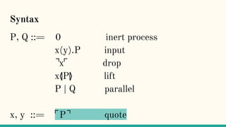
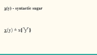
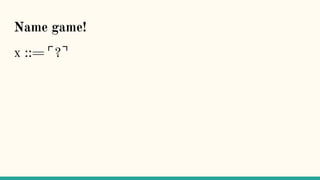
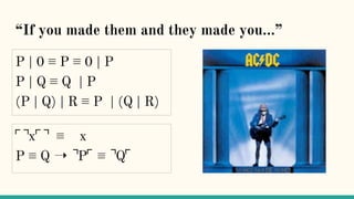
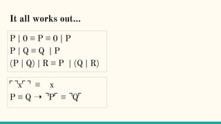
![Quoting
“Here we present a theory of an asynchronous
message-passing calculus built on a notion of
quoting. Names are quoted processes, and as such
represent the code of a process.(...) Name-passing,
then becomes a way of passing the code of a
process as a message.” [7]](https://image.slidesharecdn.com/understandingdistributedcalculiinhaskell-180304222304/85/Understanding-distributed-calculi-in-Haskell-242-320.jpg)

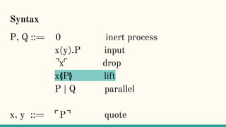
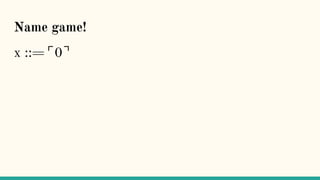
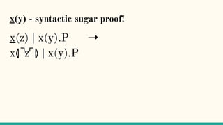
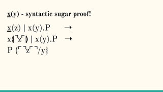
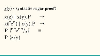
![x⦉P⦊
“Process P will be packaged up as its code, ⌜P⌝,
and ultimately made available as an output at the
port x” [7]](https://image.slidesharecdn.com/understandingdistributedcalculiinhaskell-180304222304/85/Understanding-distributed-calculi-in-Haskell-247-320.jpg)
![x⦉P⦊
“Process P will be packaged up as its code, ⌜P⌝,
and ultimately made available as an output at the
port x” [7]
“The lift operator turns out to play a role
analogous to (νx)”](https://image.slidesharecdn.com/understandingdistributedcalculiinhaskell-180304222304/85/Understanding-distributed-calculi-in-Haskell-248-320.jpg)

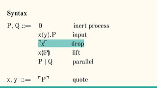
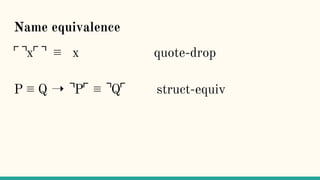
![⌝x⌜
“The ⌝x⌜ operator (...) eventually extracts the
process from a name. We say ‘eventually’ because
this extraction only happens when quoted process
is substituted into this expression.” [7]](https://image.slidesharecdn.com/understandingdistributedcalculiinhaskell-180304222304/85/Understanding-distributed-calculi-in-Haskell-251-320.jpg)
![⌝x⌜
“A consequence of this behaviour is that the ⌝x⌜ is
inert, except under an input prefix” [7]](https://image.slidesharecdn.com/understandingdistributedcalculiinhaskell-180304222304/85/Understanding-distributed-calculi-in-Haskell-252-320.jpg)

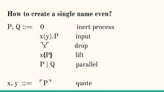
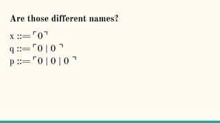
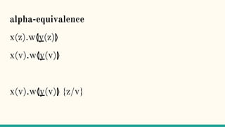
![Are those different names?
“This question leads to several intriguing and
apparently fundamental questions. Firstly, if
names have structure, what is a reasonable notion
of equality on names? How much computation, and
of what kind, should go into ascertaining equality
on names?” [7]](https://image.slidesharecdn.com/understandingdistributedcalculiinhaskell-180304222304/85/Understanding-distributed-calculi-in-Haskell-269-320.jpg)


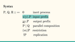
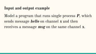
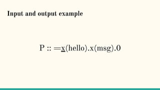
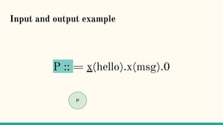
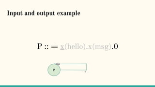
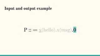
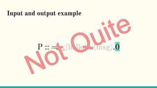
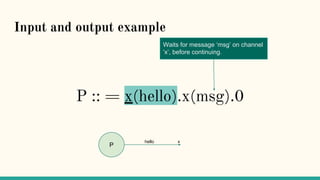
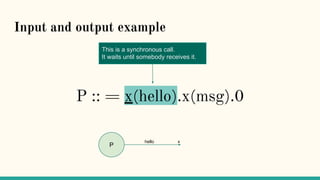
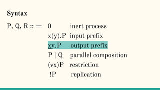
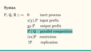
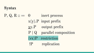
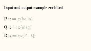
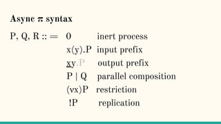
The document discusses distributed calculi and the pi-calculus in particular. It begins with an overview of the pi-calculus syntax including processes, input/output prefixes, parallel composition, restriction and replication. Examples are given to demonstrate communication between processes using input/output prefixes. Structural congruence and reduction rules are also covered. The document concludes with an example of modeling a simple ping-pong protocol in pi-calculus.