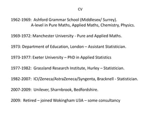
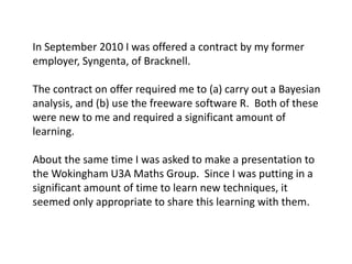
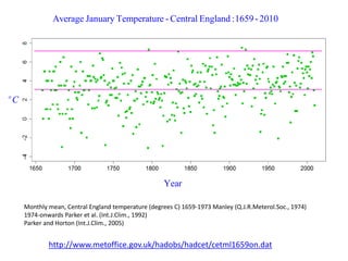
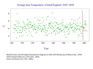
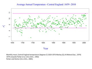
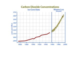
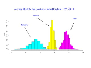
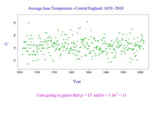
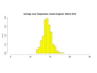
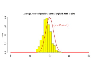
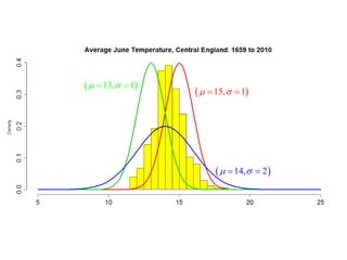
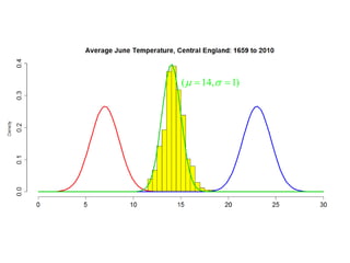
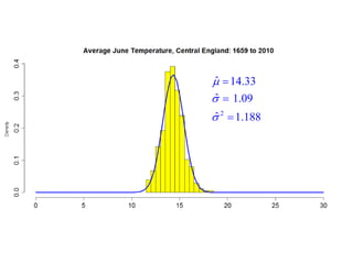
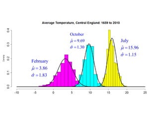
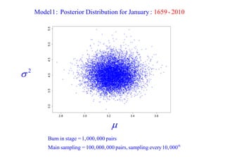
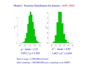
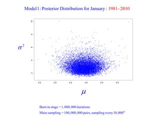
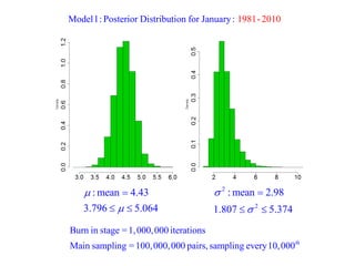
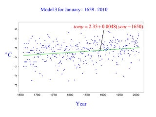
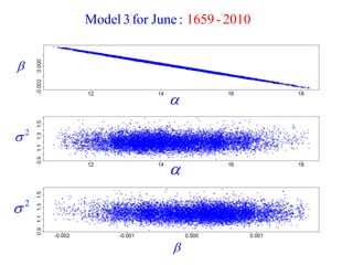
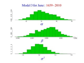
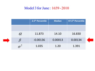
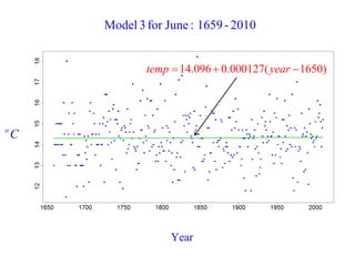
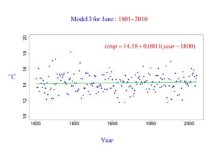
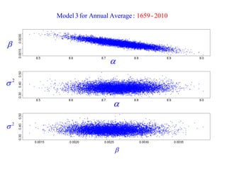
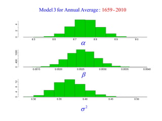
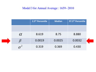
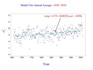
My Adventures with Bayes 
Peter Chapman 
Wokingham U3A Maths Group 
6 April 2011
Contents 
•My background 
•Motivation 
•Some data 
•The normal distribution 
•Classical inference 
•Bayes theorem 
•Who was Thomas Bayes 
•Bayesian inference 
•Some examples of Bayesian inference
WHO AM I
CV 
1962-1969: Ashford Grammar School (Middlesex/ Surrey). 
A-level in Pure Maths, Applied Maths, Chemistry, Physics. 
1969-1972: Manchester University - Pure and Applied Maths. 
1973: Department of Education, London – Assistant Statistician. 
1973-1977: Exeter University – PhD in Applied Statistics 
1977-1982: Grassland Research Institute, Hurley – Statistician. 
1982-2007: ICI/Zeneca/AstraZeneca/Syngenta, Bracknell - Statistician. 
2007-2009: Unilever, Sharnbrook, Bedfordshire. 
2009: Retired – joined Wokingham U3A – some consultancy
MOTIVATION
In September 2010 I was offered a contract by my former employer, Syngenta, of Bracknell. 
The contract on offer required me to (a) carry out a Bayesian analysis, and (b) use the freeware software R. Both of these were new to me and required a significant amount of learning. 
About the same time I was asked to make a presentation to the Wokingham U3A Maths Group. Since I was putting in a significant amount of time to learn new techniques, it seemed only appropriate to share this learning with them.
This is a presentation about Bayesian methods. Although I am using UK temperature records to illustrate methods, this is not a presentation about climate change. 
A much more thorough analysis is necessary before we can say anything substantial about climate change. 
This presentation is not about the normal distribution. Because the normal distribution is well known and easy to work with I have used it to demonstrate Bayesian methodology. The ideas presented here will translate to other, more complex, distributions.
SOME DATA
Monthly mean, Central England temperature (degrees C) 1659-1973 Manley (Q.J.R.Meterol.Soc., 1974) 
1974-onwards Parker et al. (Int.J.Clim., 1992) 
Parker and Horton (Int.J.Clim., 2005) 
Year 
oC 
Average January Temperature - Central England :1659 - 2010 
http://www.metoffice.gov.uk/hadobs/hadcet/cetml1659on.dat
Monthly mean, Central England temperature (degrees C) 1659-1973 Manley (Q.J.R.Meterol.Soc., 1974) 
1974-onwards Parker et al. (Int.J.Clim., 1992) 
Parker and Horton (Int.J.Clim., 2005) 
Year 
oC 
Average June Temperature - Central England :1659 - 2010
Monthly mean, Central England temperature (degrees C) 1659-1973 Manley (Q.J.R.Meterol.Soc., 1974) 
1974-onwards Parker et al. (Int.J.Clim., 1992) 
Parker and Horton (Int.J.Clim., 2005) 
Year 
oC 
Average Annual Temperature - Central England :1659 - 2010
Average Monthly Temperature - Central England :1659 - 2010 
January 
June 
Annual
THE NORMAL DISTRIBUTION
 2 
2 2 
2 
1 
2 
x 
e 
 
 
 
 
 
f (x | ,  2 ) 
 
  
 2 
2 2 2 
2 
1 
| , 
2 
x 
y f x e 
 
   
 
 
 
  
X 
 
2 
is called the mean 
is called the variance 
is called the standard deviation 
 
 

 
 2 
2 2 
2 
1 
Prob( ) 
2 
b x 
X b e dx 
 
 
 
 
 
 
   
X 
b 

 
 
 2 
2 
2 
2 
1 2 
2 
1 
1 
Prob( ) 
2 
b x 
b 
b X b e dx 
 
 
 
 
 
    
X 
b1 b2
 
 
 2 
2 2 
2 
1 
Prob( ) 1 
2 
x 
X e dx 
 
 
 
  
 
 
       
X
2 
 
 2 
2 2 
2 
1 
Prob( ) 0.66 ( ) 
2 
x 
X e dx approx 
   
 
  
    
 
  
 
 
       
X
4 
 
 2 
2 
2 
2 
2 
2 
1 
Prob( 2 2 ) 0.95 ( ) 
2 
x 
X e dx approx 
   
 
  
    
 
  
 
 
       
X
6 
 
 2 
2 
3 
2 
2 
3 
1 
Prob( 3 3 ) 0.99( ) 
2 
x 
X e dx approx 
   
 
  
    
 
  
 
 
       
X
 2 
2 2 
2 
1 
Prob( ) 
2 
x x 
X x e dx 
 
 
 
 
 
 
   
1.0 
0.0 
b 
 2 
2 2 1 
Prob( ) 
2 
b x 
X b e dx 
 
 
 
 
 
 
   
X
  
 2 
2 
x-μ 
- 
2 2σ 
2 
(Probability) 
1 
f x | μ,σ = e is called a Density F . 
2πσ 
unction (PDF) 
 2 
2 2 2 
2 
1 
( | , ) is called a Cumulative Distribution Funcion ( . 
2 
CDF) 
x x 
F x e dx 
 
   
 
 
 
 
  
2 Vertical line indicates a distribution of x conditional on the values of μ and σ
CLASSICAL INFERENCE
We have some data..............and we believe that the data derives from 
a normal distribution. 
Fundamental principle : the parameters, μ and σ in our case, 
are fixed or constant. 
. 
Our objective is therefore to estimate μ and σ2............μˆ and2 σˆ . 
We also want to know how precise the parameter estimates are........ 
.......... so we need to compute confidence intervals. 
2 
2 2 
At this stage we can compute ( | , )for a variety of values 
of μ and σ , but we do not know the correct values for μ and σ . 
f x  
Year 
oC 
Average June Temperature - Central England :1659 - 2010 
2 I am going to guess that μ = 15 and σ = 1 (σ = 1)
15,1
 15, 1 
 13, 1 
 14,  2
 2 
2 
i 
- 
- 
2 22 
2 
We have 352 values of temperature, t ,where i =1659 to 2010. 
1 
We can compute ( | , ) for any value of and we like. 
2 
ti 
i f t e 
 
     
 
 
2010 
2 
1659 
2 
i In the classical approach we compute ( | , ) for all t , i =1659 2010. 
then multiply then together ( | , ) ( | , ). i 
i 
i 
L 
f t 
t   f t  
  
 
 
 
  
This is called the likelihood. 
2 We then find the values of  and  that maximise the likelihood. 
2 We call these maximum- likelihood estimates : ˆ and ˆ .
(7,1.5)
(23,1.5)
(14,1)
 2 
2 
2010 
2 2 
2 
1659 
1 
( , ) 
2 
ti 
i 
L e 
 
   
 
 
 
 
  
  
2010 
* 2 2 2 
2 
1659 
352 352 1 
( , ) log (2 ) log ( ) ( ) 
2 2 2 e e e i 
i 
L Log L     t  
  
       
* 2010 
2 
2 
1659 
1 
( - ) 0 i 
i 
L 
t  
   
 
  
  
2010 
1659 
1 
ˆ 
352 i 
i 
 t t 
 
   
* 2010 
2 
2 2 4 
1659 
352 1 1 
( - ) 0 
2 2 i 
i 
L 
t  
    
 
    
  
2010 
2 2 
1659 
1 
ˆ ( - ) 
352 i 
i 
 t t 
 
 
2 ˆ14.33 ˆ 1.09 ˆ1.188      
July 
ˆ 15.96 
ˆ 1.15 
 
 
 
 
February 
ˆ 3.86 
ˆ 1.83 
 
 
 
 
October 
ˆ 9.69 
ˆ 1.30 
 
 
 

Confidence Intervals 
Beyond the scope of this talk
BAYES THEOREM
Q = set of people tested for disease 
D = subset of people who have disease 
D = subset of people who do not have disease 
T = subset of people who test positive 
T = set of people who do not test positive 
D+D = T + T = Q 
P(D) = probability that an individual has the disease 
P(D| T) = probability that an individual has a disease given that they have tested positive 
P(T) = probability that an individual tests positive 
P(T | D) = probability that an individual tests positive given that they have the disease 
( | ) ( ) 
( | ) 
( ) 
P T D P D 
P D T 
P T 
Bayes Theorem: 
Sum 
9,900 
10,000 
19,900 
100 
9,980,000 
9,980,100 
Sum 
10,000 
9,990,000 
10,000,000 
D D 
T 
T
9,900 10000 19,900 
100 9,980,000 9,980,100 
10,000 9,990,000 10,000,000 
D D 
T 
T 
10000 
( ) 0.001 
10000000 
P D   
19900 
( ) 0.00199 
10000000 
P T   
( ) and ( P T P D) are marginal probabilities
9,900 10000 19,900 
100 9,980,000 9,980,100 
10,000 9,990,000 10,000,000 
D D 
T 
T 
9900 
( | ) 0.99 
10000 
P T D   
P(D| T) are P(T | D) are 
conditional probabilities 
( | ) ( ) 
( | ) 
( ) 
P T D P D 
P D T 
P T 
 
0.99*0.001 
0.00199 
 
0.00099 
0.00199 
 
9900 
19900 
  0.497487 
9900 
( | ) 0.497487 
19900 
P D T  
BAYESIAN INFERENCE
A fundamental assumption of Bayesian inference is that the unknown parameters are variables. 
2 For the normal distribution this means that μ and σ are variables, not constants. 
2 2 
2 2 2 
If we apply Bayes theorem to the normal density function we get : 
( | , ) ( , ) 
( , | ) ( | , ) ( , ) 
( ) 
L t f 
f t L t f 
f t 
    
        
Posterior 
Distribution 
Likelihood Prior 
Distribution 
Data
For many years Bayesian analysis was a theoretical academic pastime. 
This was because the mathematics was very difficult. 
Analytic solutions for the posterior often involved complex multiple integrals. 
One of the few that can be solved is the normal distribution with uniform priors. 
2010 
, 
1659 
1 
352 i 
i 
t t 
 
  
  
  
2010 
2 2 
1659 
1 
, - . 
352 -1) i 
i 
and s t t 
 
  
In what follows :
If μ and logσ follow independent uniform prior distributions, then : 
2 
2 
1 
f (, ) , so 
 
 
     2 
2 2 
2 
352 
1 1 
exp 352 1 352 , 
2 
1 
s t 
   
 
            
  
  
  
 
    
2010 
2 
3 2 2 
1 59 
5 2 
6 
1 1 
e 
2 
p , 
1 
x i 
i 
t  
    
    
    
 
  
    
 
 
  
  
 
  
2010 
2 
2 
16 
2 
59 
1 1 
ex , 
2 
1 
p i 
i 
t  
    
    
    
    
 
  
  
  
 
2 2 2 f (, |T)  L(T |, ) f (, ) 
      2 
352 2 
2 
2 2 
1 
exp 35 
1 1 
exp 352 2 
1 
2 
, 
2 
1 s t 
  
 
  
     
  
      
  
 
 
 
  
 
  
    
  
    2 
352 2 
2 
2 
1 1 
exp 352 1 , 
2 352 
1 
s N t , 
 
 
  
  
    
 
   
 
 
  
 
 
 
 

    2 2 2 
: 
( , | ) | , | , 
We need to factorise the posterior as follows 
f   T  f   T  f  T 
and it can be shown that that : 
2 
2 | , , , 
352 
T N t 
 
  
  
  
  
2 2 2  |T Inv (352 1, s ), and 
2 
1 | , . 
352 n 
s 
 T t t  
  
  
  
Marginal posterior for μ 
2 Marginal posterior for σ 
Conditional posterior for  
2 2 f ( |T) f ( , |T)d 
 
      
2 
2 2 f ( |T) f ( , |T)d 
 
     
MARKOV CHAIN MONTE-CARLO AND THE METROPOLIS METHOD
2 2 
2 2 2 
Set up the Bayesian posterior : 
( | , ) ( , ) 
( , | ) ( | , ) 
( 
( , ) 
) 
L 
L T f 
f T 
f 
T f 
y 
   
   
 
     
  2 
2010 
2 
2 
1659 
In our case it takes the following form: 
1 1 
exp 
2 
1 
, i 
i 
t  
    
    
    
  
  
 
  
 

2 2 
0 0 Select initial values,  and  , for  and  . 
2 2 
0 1 0 1 Introduce jump functions :  and   
2 
1 1 
2 
0 0 
( , | ) 
Compute = R. 
( , | ) 
f T 
f T 
  
  
  
  
  
Sample a single random value Q from a UnifoUrm distribution (0,1) 
2 2 2 
1 1 1 1 0 0 If Q  min(1, R) keep ( , ) else ............( , ) ( , ) 
2 2 2 
0 0 1 1 2 2 
2 2 2 
1 1 
Continue doing this ( , ) ( , ) ( , ) 
( , ) ( , ) ( , ) n n n n big big 
      
        
   
   
This results in a random joint sample from the posterior distribution.
 
Posterior Distribution 
n 1 n   
  1 | n f  T   |  n f  T 
1 
1 
( | ) 
= R >1 Q so keep 
( | ) 
n 
n 
n 
f T 
f T 
 
 
 
 
 
  
   
 
 
Posterior Distribution 
n 1  n   
 |  n f  T 
  1 | n f  T  
1 
1 
1 
( | ) 
= R <1.........if keep 
( | ) 
so keep with probability = R 
n 
n 
n 
n 
f T 
Q R 
f T 
 
 
 
 
 
 
 
  
   
 
  2 , n n   
  2 
1 1 , n n     Jump Function 
2 
n 1 n rnorm(0, Z )    
2 2 2 
1 (0, ) n n W   rnorm    
A COMPARISON OF THREE MODELS
  
  
  
  
  
  
2 
2 
2 
2 2 
2 2 
2 
2 2 2 
2 2 
1 
| , 
2 
1 
| , , , 
2 
t 
t 
f t e 
f t e 
 
 
  
  
  
 
    
   
 
 
  
 
 
 
 
 
  
 2 
2 2 2 
2 
1 
| , 
2 
t 
f t e 
 
   
 
 
 
Model 1  for all years. 
Model 2 
for earlier years 
for later years 
Model 3   
  2 
2 2 2 
2 
1 
| , , 
2 
t t 
f t e 
  
    
 
  
 
 
i.e.    t
    
    
2 2 
2 2 2 2 
| , , 
| , , , , 
f t N 
f t N 
    
        
    2 2 Model 1 f t |,  N , for all years. 
Model 2 
for earlier years 
for later years 
Model 3     2 2 f t | , ,  N   t, i.e.    t
for earlier years 
for later years 
    
    
2 2 
2 2 2 2 
| , , 
| , , , , 
f t N 
f t N 
    
        
Model 2 
for earlier years 
for later years 
    
    
2 2 
2 2 
| , , 
| , , 
early early early early 
late late late late 
f t N 
f t N 
    
    
Model 2 
Is the same as 
2 2 2 where and late early late early       
Model 1 
  
 2 
2 2 2 
2 
1 
| , 
2 
t 
f t e 
 
   
 
 
 
 
    2 2 f t |,  N ,
 
2  
MCMC Done Very Badly : June : 1659 - 2010 
  2 
0 0  , 
Jumps Too Small 
High correlation between consecutive pairs of sample values. 
Posterior Distribution
Solution 
    2 2 
Better starting values 0 , 0  maximum likelihood estimates ˆ ,ˆ 
Burn in sampling phase that is discarded 
Main phase with infrequent sampling - e.g. every 10,000 pair th
2  
th 
Burn in stage =1,000,000 pairs 
Main sampling =100,000,000 pairs, sampling every 10,000 
 
Model 1: Posterior Distribution for June : 1659 - 2010
th 
Burn in stage =1,000,000 pairs 
Main sampling =100,000,000 pairs, sampling every 10,000 
Model 1: Posterior Distribution for June : 1659 - 2010 
:mean 14.33 
14.213 4.440 
 
 
 
  
2 
2 
:mean 1.20 
1.034 1.389 
 
 
 
 
2  
th 
Burn in stage =1,000,000 pairs 
Main sampling =100,000,000 pairs, sampling every 10,000 
Model 1: Posterior Distribution for January : 1659 - 2010 

Model 1: Posterior Distribution for January : 1659 - 2010 
1,000,000 
100,000,000 , 10000th 
Burn in stage iterations 
Main sampling pairs sampling every 
 
 
2 
2 
: mean 4.02 
3.467 4.691 
 
 
 
  
: mean 3.23 
3.022 3.442 
 
 
 
 
Model 1: Posterior Distribution for January : 1981- 2010 
th 
Burn in stage =1,000,000 iterations 
Main sampling =100,000,000 pairs, sampling every 10,000 
 
2 
th 
Burn in stage =1,000,000 iterations 
Main sampling =100,000,000 pairs, sampling every 10,000 
Model 1: Posterior Distribution for January : 1981- 2010 
:mean 4.43 
3.796 5.064 
 
 
 
  
2 
2 
:mean 2.98 
1.807 5.374 
 
 
 
 
Model 1:Distribution for January : 1881-1910 
th 
Burn in stage =1,000,000 iterations 
Main sampling =100,000,000 pairs, sampling every 10,000 
 
2 
th 
Burn in stage =1,000,000 iterations 
Main sampling =100,000,000 pairs, sampling every 10,000 
Model 1:Distribution for January : 1881-1910 
:mean 3.50 
2.857 4.144 
 
 
 
  
2 
2 
:mean 3.17 
1.996 5.893 
 
 
 
 
o January Average Temperature , C,Central England 
18811910 1981 2010
o Average January Temperature, C 
17811810 18811910 1981 2010 
ˆ  2.87 ˆ  3.49 ˆ  4.44
o Average June Temperature, C 
17811810 18811910 1981 2010 
ˆ 14.54 ˆ 14.11 ˆ 14.48
Model 2 
    
    
2 2 
2 2 2 2 
| , , 
| , , , , 
f t N 
f t N 
    
        
  
  
  
  
  
  
2 
2 
2 
2 2 
2 2 
2 
2 2 2 
2 2 
1 
| , 
2 
1 
| , , , 
2 
t 
t 
f t e 
f t e 
 
 
  
  
  
 
    
   
 
 
  
 
 
 
 

th 
Burn in stage =10,000,000 iterations 
Main stage =100,000,000 sets of four, sampling every 10,000 
Model 2 for January : (1881,1910) and (1981,2010) 
 
 
 
2  
2  
2  
 
 
 2  
2  2 
Model 2 for January : (1881,1910) and (1981,2010) 
 2  
2  
2.5th Percentile Median 97.5th Percentile 
2.868 3.49 4.119 
0.079 0.94 1.851 
1.942 3.03 4.686 
-1.588 0.07 2.276 
 
 
2  
2  
Model 2 for January : (1881,1910) and (1981,2010)
th 
Burn in stage =10,000,000 iterations 
Main stage =100,000,000 sets of four, sampling every 10,000 
Model 2 for June : (1881,1910) and (1981,2010)
Model 2 for June : (1881,1910) and (1981,2010) 
 2  
 2 
2.5th Percentile Median 97.5th Percentile 
13.745 14.10 14.464 
-0.122 0.38 0.866 
0.641 0.98 1.515 
-0.587 -0.09 0.778 
 
 
2  
2  
Model 2 for June : (1881,1910) and (1981,2010)
Model 3 
  
  2 
2 2 2 
2 
1 
| , , 
2 
t t 
f t e 
  
    
 
  
 
 
    2 2 f t | , ,  N   t,
Model 3 for January : 1659 - 2010 
 
 
2  
 
2  

Model 3 for January : 1659 - 2010 
 
 
2 
2.5th Percentile Median 97.5th Percentile 
1.921 2.35 2.770 
0.0028 0.0048 0.0068 
1.271 3.790 4.411 
Model 3 for January : 1659 - 2010 
 
 
2 
Model 3 for January : 1659 - 2010 
oC 
Year 
temp  2.35  0.0048( year 1650)
Model 3 for June : 1659 - 2010 
 
 
 
 
2  
2 
Model 3 for June : 1659 - 2010 
 
 
2 
2.5th Percentile Median 97.5th Percentile 
11.873 14.10 16.830 
-0.00136 0.00013 0.00134 
1.035 1.20 1.391 
Model 3 for June : 1659 - 2010 
 
 
2 
Year 
Model 3 for June : 1659 - 2010 
oC 
temp 14.096  0.000127( year 1650)
Model 3 for June : 1801- 2010 
Year 
oC 
temp 14.18  0.0011( year 1800)
Model 3 for Annual Average : 1659 - 2010 
 
 
 
 
2  
2 
2  
 
 
Model 3 for Annual Average : 1659 - 2010
2.5th Percentile Median 97.5th Percentile 
8.619 8.75 8.880 
0.0019 0.0025 0.0032 
0.319 0.369 0.430 
 
 
2  
Model 3 for Annual Average : 1659 - 2010
Model 3 for Annual Average : 1659 - 2010 
oC 
Year 
temp  8.75  0.0025( year 1650)
THOMAS BAYES
Rev. Thomas Bayes (1702-1761) 
His friend Richard Price edited and presented his work in 1763, after Bayes' death, as An Essay towards solving a Problem in the Doctrine of Chances. 
The French mathematician Pierre-Simon Laplace reproduced and extended Bayes' results in 1774, apparently quite unaware of Bayes' work. 
It is speculated that Bayes was elected as a Fellow of the Royal Society in 1742 on the strength of the Introduction to the Doctrine of Fluxions, as he is not known to have published any other mathematical works during his lifetime. 
It has been suggested that Bayes' theorem, as we now call it, was discovered by Nicholas Saunderson some time before Bayes. This is disputed.
Comments in place of Conclusions: Bayesian Inference 
•This presentation was not about the Normal distribution. 
•The Normal distribution was used to illustrate the methods. 
•For the problems discussed here Bayesian inference offers few advantages over classical. 
•For more complex problems, Bayesian inference offers big advantages. 
•Prior to 1990 or so, Bayesian inference was a partially academic subject. 
•The advent of MCMC and fast computers has made Bayesian inference a significant player in the world of data analysis. 
•The numbers of PhDs in statistics is small and getting smaller but most of them are absorbed in Bayesian issues. 
•Bayesian approaches are now commonplace.
Comments: Climate Change 
•This presentation was not about climate change. 
•A more thorough analysis is required before we can say anything substantial about climate change. 
•The results of a limited analysis so far indicate, for Central England, that summers are not getting warmer. The range of average summer temperatures that we see today is similar to that seen in the past. 
•The range of average winter temperatures seems to be narrower than in the past with an absence of very cold months in recent years. 
•This effect could, of course, be a result of thermometers being placed in urban areas. 
•The statistically significant increase in annual average temperature may be caused may be caused by increasing average winter temperatures.

Introduction to Bayesian Inference

  • 1.
    My Adventures withBayes Peter Chapman Wokingham U3A Maths Group 6 April 2011
  • 2.
    Contents •My background •Motivation •Some data •The normal distribution •Classical inference •Bayes theorem •Who was Thomas Bayes •Bayesian inference •Some examples of Bayesian inference
  • 3.
  • 4.
    CV 1962-1969: AshfordGrammar School (Middlesex/ Surrey). A-level in Pure Maths, Applied Maths, Chemistry, Physics. 1969-1972: Manchester University - Pure and Applied Maths. 1973: Department of Education, London – Assistant Statistician. 1973-1977: Exeter University – PhD in Applied Statistics 1977-1982: Grassland Research Institute, Hurley – Statistician. 1982-2007: ICI/Zeneca/AstraZeneca/Syngenta, Bracknell - Statistician. 2007-2009: Unilever, Sharnbrook, Bedfordshire. 2009: Retired – joined Wokingham U3A – some consultancy
  • 5.
  • 6.
    In September 2010I was offered a contract by my former employer, Syngenta, of Bracknell. The contract on offer required me to (a) carry out a Bayesian analysis, and (b) use the freeware software R. Both of these were new to me and required a significant amount of learning. About the same time I was asked to make a presentation to the Wokingham U3A Maths Group. Since I was putting in a significant amount of time to learn new techniques, it seemed only appropriate to share this learning with them.
  • 7.
    This is apresentation about Bayesian methods. Although I am using UK temperature records to illustrate methods, this is not a presentation about climate change. A much more thorough analysis is necessary before we can say anything substantial about climate change. This presentation is not about the normal distribution. Because the normal distribution is well known and easy to work with I have used it to demonstrate Bayesian methodology. The ideas presented here will translate to other, more complex, distributions.
  • 8.
  • 9.
    Monthly mean, CentralEngland temperature (degrees C) 1659-1973 Manley (Q.J.R.Meterol.Soc., 1974) 1974-onwards Parker et al. (Int.J.Clim., 1992) Parker and Horton (Int.J.Clim., 2005) Year oC Average January Temperature - Central England :1659 - 2010 http://www.metoffice.gov.uk/hadobs/hadcet/cetml1659on.dat
  • 10.
    Monthly mean, CentralEngland temperature (degrees C) 1659-1973 Manley (Q.J.R.Meterol.Soc., 1974) 1974-onwards Parker et al. (Int.J.Clim., 1992) Parker and Horton (Int.J.Clim., 2005) Year oC Average June Temperature - Central England :1659 - 2010
  • 11.
    Monthly mean, CentralEngland temperature (degrees C) 1659-1973 Manley (Q.J.R.Meterol.Soc., 1974) 1974-onwards Parker et al. (Int.J.Clim., 1992) Parker and Horton (Int.J.Clim., 2005) Year oC Average Annual Temperature - Central England :1659 - 2010
  • 14.
    Average Monthly Temperature- Central England :1659 - 2010 January June Annual
  • 15.
  • 16.
     2 22 2 1 2 x e      f (x | ,  2 ) 
  • 17.
        2 2 2 2 2 1 | , 2 x y f x e          X  2 is called the mean is called the variance is called the standard deviation   
  • 18.
      2 2 2 2 1 Prob( ) 2 b x X b e dx          X b 
  • 19.
      2 2 2 2 1 2 2 1 1 Prob( ) 2 b x b b X b e dx          X b1 b2
  • 20.
      2 2 2 2 1 Prob( ) 1 2 x X e dx               X
  • 21.
    2  2 2 2 2 1 Prob( ) 0.66 ( ) 2 x X e dx approx                       X
  • 22.
    4  2 2 2 2 2 2 1 Prob( 2 2 ) 0.95 ( ) 2 x X e dx approx                       X
  • 23.
    6  2 2 3 2 2 3 1 Prob( 3 3 ) 0.99( ) 2 x X e dx approx                       X
  • 24.
     2 22 2 1 Prob( ) 2 x x X x e dx          1.0 0.0 b  2 2 2 1 Prob( ) 2 b x X b e dx          X
  • 25.
      2 2 x-μ - 2 2σ 2 (Probability) 1 f x | μ,σ = e is called a Density F . 2πσ unction (PDF)  2 2 2 2 2 1 ( | , ) is called a Cumulative Distribution Funcion ( . 2 CDF) x x F x e dx           2 Vertical line indicates a distribution of x conditional on the values of μ and σ
  • 26.
  • 27.
    We have somedata..............and we believe that the data derives from a normal distribution. Fundamental principle : the parameters, μ and σ in our case, are fixed or constant. . Our objective is therefore to estimate μ and σ2............μˆ and2 σˆ . We also want to know how precise the parameter estimates are........ .......... so we need to compute confidence intervals. 2 2 2 At this stage we can compute ( | , )for a variety of values of μ and σ , but we do not know the correct values for μ and σ . f x  
  • 28.
    Year oC AverageJune Temperature - Central England :1659 - 2010 2 I am going to guess that μ = 15 and σ = 1 (σ = 1)
  • 30.
  • 31.
     15, 1  13, 1  14,  2
  • 32.
     2 2 i - - 2 22 2 We have 352 values of temperature, t ,where i =1659 to 2010. 1 We can compute ( | , ) for any value of and we like. 2 ti i f t e         2010 2 1659 2 i In the classical approach we compute ( | , ) for all t , i =1659 2010. then multiply then together ( | , ) ( | , ). i i i L f t t   f t         This is called the likelihood. 2 We then find the values of  and  that maximise the likelihood. 2 We call these maximum- likelihood estimates : ˆ and ˆ .
  • 34.
  • 35.
  • 36.
  • 37.
     2 2 2010 2 2 2 1659 1 ( , ) 2 ti i L e             2010 * 2 2 2 2 1659 352 352 1 ( , ) log (2 ) log ( ) ( ) 2 2 2 e e e i i L Log L     t           * 2010 2 2 1659 1 ( - ) 0 i i L t          2010 1659 1 ˆ 352 i i  t t     * 2010 2 2 2 4 1659 352 1 1 ( - ) 0 2 2 i i L t             2010 2 2 1659 1 ˆ ( - ) 352 i i  t t   
  • 38.
    2 ˆ14.33 ˆ1.09 ˆ1.188      
  • 39.
    July ˆ 15.96 ˆ 1.15     February ˆ 3.86 ˆ 1.83     October ˆ 9.69 ˆ 1.30    
  • 40.
    Confidence Intervals Beyondthe scope of this talk
  • 41.
  • 42.
    Q = setof people tested for disease D = subset of people who have disease D = subset of people who do not have disease T = subset of people who test positive T = set of people who do not test positive D+D = T + T = Q P(D) = probability that an individual has the disease P(D| T) = probability that an individual has a disease given that they have tested positive P(T) = probability that an individual tests positive P(T | D) = probability that an individual tests positive given that they have the disease ( | ) ( ) ( | ) ( ) P T D P D P D T P T Bayes Theorem: 
  • 43.
    Sum 9,900 10,000 19,900 100 9,980,000 9,980,100 Sum 10,000 9,990,000 10,000,000 D D T T
  • 44.
    9,900 10000 19,900 100 9,980,000 9,980,100 10,000 9,990,000 10,000,000 D D T T 10000 ( ) 0.001 10000000 P D   19900 ( ) 0.00199 10000000 P T   ( ) and ( P T P D) are marginal probabilities
  • 45.
    9,900 10000 19,900 100 9,980,000 9,980,100 10,000 9,990,000 10,000,000 D D T T 9900 ( | ) 0.99 10000 P T D   P(D| T) are P(T | D) are conditional probabilities ( | ) ( ) ( | ) ( ) P T D P D P D T P T  0.99*0.001 0.00199  0.00099 0.00199  9900 19900   0.497487 9900 ( | ) 0.497487 19900 P D T  
  • 46.
  • 47.
    A fundamental assumptionof Bayesian inference is that the unknown parameters are variables. 2 For the normal distribution this means that μ and σ are variables, not constants. 2 2 2 2 2 If we apply Bayes theorem to the normal density function we get : ( | , ) ( , ) ( , | ) ( | , ) ( , ) ( ) L t f f t L t f f t             Posterior Distribution Likelihood Prior Distribution Data
  • 48.
    For many yearsBayesian analysis was a theoretical academic pastime. This was because the mathematics was very difficult. Analytic solutions for the posterior often involved complex multiple integrals. One of the few that can be solved is the normal distribution with uniform priors. 2010 , 1659 1 352 i i t t        2010 2 2 1659 1 , - . 352 -1) i i and s t t    In what follows :
  • 49.
    If μ andlogσ follow independent uniform prior distributions, then : 2 2 1 f (, ) , so        2 2 2 2 352 1 1 exp 352 1 352 , 2 1 s t                            2010 2 3 2 2 1 59 5 2 6 1 1 e 2 p , 1 x i i t                              2010 2 2 16 2 59 1 1 ex , 2 1 p i i t                          2 2 2 f (, |T)  L(T |, ) f (, )       2 352 2 2 2 2 1 exp 35 1 1 exp 352 2 1 2 , 2 1 s t                                       2 352 2 2 2 1 1 exp 352 1 , 2 352 1 s N t ,                       
  • 50.
       2 2 2 : ( , | ) | , | , We need to factorise the posterior as follows f   T  f   T  f  T and it can be shown that that : 2 2 | , , , 352 T N t          2 2 2  |T Inv (352 1, s ), and 2 1 | , . 352 n s  T t t        Marginal posterior for μ 2 Marginal posterior for σ Conditional posterior for  2 2 f ( |T) f ( , |T)d        2 2 2 f ( |T) f ( , |T)d       
  • 51.
    MARKOV CHAIN MONTE-CARLOAND THE METROPOLIS METHOD
  • 52.
    2 2 22 2 Set up the Bayesian posterior : ( | , ) ( , ) ( , | ) ( | , ) ( ( , ) ) L L T f f T f T f y               2 2010 2 2 1659 In our case it takes the following form: 1 1 exp 2 1 , i i t                      
  • 53.
    2 2 00 Select initial values,  and  , for  and  . 2 2 0 1 0 1 Introduce jump functions :  and   2 1 1 2 0 0 ( , | ) Compute = R. ( , | ) f T f T           Sample a single random value Q from a UnifoUrm distribution (0,1) 2 2 2 1 1 1 1 0 0 If Q  min(1, R) keep ( , ) else ............( , ) ( , ) 2 2 2 0 0 1 1 2 2 2 2 2 1 1 Continue doing this ( , ) ( , ) ( , ) ( , ) ( , ) ( , ) n n n n big big                     This results in a random joint sample from the posterior distribution.
  • 54.
     Posterior Distribution n 1 n     1 | n f  T   |  n f  T 1 1 ( | ) = R >1 Q so keep ( | ) n n n f T f T            
  • 55.
     Posterior Distribution n 1  n    |  n f  T   1 | n f  T  1 1 1 ( | ) = R <1.........if keep ( | ) so keep with probability = R n n n n f T Q R f T              
  • 56.
      2, n n     2 1 1 , n n     Jump Function 2 n 1 n rnorm(0, Z )    2 2 2 1 (0, ) n n W   rnorm    
  • 57.
    A COMPARISON OFTHREE MODELS
  • 58.
               2 2 2 2 2 2 2 2 2 2 2 2 2 1 | , 2 1 | , , , 2 t t f t e f t e                             2 2 2 2 2 1 | , 2 t f t e        Model 1  for all years. Model 2 for earlier years for later years Model 3     2 2 2 2 2 1 | , , 2 t t f t e            i.e.    t
  • 59.
           2 2 2 2 2 2 | , , | , , , , f t N f t N                 2 2 Model 1 f t |,  N , for all years. Model 2 for earlier years for later years Model 3     2 2 f t | , ,  N   t, i.e.    t
  • 60.
    for earlier years for later years         2 2 2 2 2 2 | , , | , , , , f t N f t N             Model 2 for earlier years for later years         2 2 2 2 | , , | , , early early early early late late late late f t N f t N         Model 2 Is the same as 2 2 2 where and late early late early       
  • 61.
    Model 1   2 2 2 2 2 1 | , 2 t f t e             2 2 f t |,  N ,
  • 62.
     2  MCMC Done Very Badly : June : 1659 - 2010   2 0 0  , Jumps Too Small High correlation between consecutive pairs of sample values. Posterior Distribution
  • 63.
    Solution    2 2 Better starting values 0 , 0  maximum likelihood estimates ˆ ,ˆ Burn in sampling phase that is discarded Main phase with infrequent sampling - e.g. every 10,000 pair th
  • 64.
    2  th Burn in stage =1,000,000 pairs Main sampling =100,000,000 pairs, sampling every 10,000  Model 1: Posterior Distribution for June : 1659 - 2010
  • 65.
    th Burn instage =1,000,000 pairs Main sampling =100,000,000 pairs, sampling every 10,000 Model 1: Posterior Distribution for June : 1659 - 2010 :mean 14.33 14.213 4.440      2 2 :mean 1.20 1.034 1.389     
  • 66.
    2  th Burn in stage =1,000,000 pairs Main sampling =100,000,000 pairs, sampling every 10,000 Model 1: Posterior Distribution for January : 1659 - 2010 
  • 67.
    Model 1: PosteriorDistribution for January : 1659 - 2010 1,000,000 100,000,000 , 10000th Burn in stage iterations Main sampling pairs sampling every   2 2 : mean 4.02 3.467 4.691      : mean 3.23 3.022 3.442     
  • 68.
    Model 1: PosteriorDistribution for January : 1981- 2010 th Burn in stage =1,000,000 iterations Main sampling =100,000,000 pairs, sampling every 10,000  2 
  • 69.
    th Burn instage =1,000,000 iterations Main sampling =100,000,000 pairs, sampling every 10,000 Model 1: Posterior Distribution for January : 1981- 2010 :mean 4.43 3.796 5.064      2 2 :mean 2.98 1.807 5.374     
  • 70.
    Model 1:Distribution forJanuary : 1881-1910 th Burn in stage =1,000,000 iterations Main sampling =100,000,000 pairs, sampling every 10,000  2 
  • 71.
    th Burn instage =1,000,000 iterations Main sampling =100,000,000 pairs, sampling every 10,000 Model 1:Distribution for January : 1881-1910 :mean 3.50 2.857 4.144      2 2 :mean 3.17 1.996 5.893     
  • 72.
    o January AverageTemperature , C,Central England 18811910 1981 2010
  • 73.
    o Average JanuaryTemperature, C 17811810 18811910 1981 2010 ˆ  2.87 ˆ  3.49 ˆ  4.44
  • 74.
    o Average JuneTemperature, C 17811810 18811910 1981 2010 ˆ 14.54 ˆ 14.11 ˆ 14.48
  • 75.
    Model 2        2 2 2 2 2 2 | , , | , , , , f t N f t N                         2 2 2 2 2 2 2 2 2 2 2 2 2 1 | , 2 1 | , , , 2 t t f t e f t e                         
  • 76.
    th Burn instage =10,000,000 iterations Main stage =100,000,000 sets of four, sampling every 10,000 Model 2 for January : (1881,1910) and (1981,2010)    2  2  2     2  2  2 
  • 77.
    Model 2 forJanuary : (1881,1910) and (1981,2010)  2  2  
  • 78.
    2.5th Percentile Median97.5th Percentile 2.868 3.49 4.119 0.079 0.94 1.851 1.942 3.03 4.686 -1.588 0.07 2.276   2  2  Model 2 for January : (1881,1910) and (1981,2010)
  • 79.
    th Burn instage =10,000,000 iterations Main stage =100,000,000 sets of four, sampling every 10,000 Model 2 for June : (1881,1910) and (1981,2010)
  • 80.
    Model 2 forJune : (1881,1910) and (1981,2010)  2   2 
  • 81.
    2.5th Percentile Median97.5th Percentile 13.745 14.10 14.464 -0.122 0.38 0.866 0.641 0.98 1.515 -0.587 -0.09 0.778   2  2  Model 2 for June : (1881,1910) and (1981,2010)
  • 82.
    Model 3    2 2 2 2 2 1 | , , 2 t t f t e                2 2 f t | , ,  N   t,
  • 83.
    Model 3 forJanuary : 1659 - 2010   2   2  
  • 84.
    Model 3 forJanuary : 1659 - 2010   2 
  • 85.
    2.5th Percentile Median97.5th Percentile 1.921 2.35 2.770 0.0028 0.0048 0.0068 1.271 3.790 4.411 Model 3 for January : 1659 - 2010   2 
  • 86.
    Model 3 forJanuary : 1659 - 2010 oC Year temp  2.35  0.0048( year 1650)
  • 87.
    Model 3 forJune : 1659 - 2010     2  2 
  • 88.
    Model 3 forJune : 1659 - 2010   2 
  • 89.
    2.5th Percentile Median97.5th Percentile 11.873 14.10 16.830 -0.00136 0.00013 0.00134 1.035 1.20 1.391 Model 3 for June : 1659 - 2010   2 
  • 90.
    Year Model 3for June : 1659 - 2010 oC temp 14.096  0.000127( year 1650)
  • 91.
    Model 3 forJune : 1801- 2010 Year oC temp 14.18  0.0011( year 1800)
  • 92.
    Model 3 forAnnual Average : 1659 - 2010     2  2 
  • 93.
    2    Model 3 for Annual Average : 1659 - 2010
  • 94.
    2.5th Percentile Median97.5th Percentile 8.619 8.75 8.880 0.0019 0.0025 0.0032 0.319 0.369 0.430   2  Model 3 for Annual Average : 1659 - 2010
  • 95.
    Model 3 forAnnual Average : 1659 - 2010 oC Year temp  8.75  0.0025( year 1650)
  • 96.
  • 97.
    Rev. Thomas Bayes(1702-1761) His friend Richard Price edited and presented his work in 1763, after Bayes' death, as An Essay towards solving a Problem in the Doctrine of Chances. The French mathematician Pierre-Simon Laplace reproduced and extended Bayes' results in 1774, apparently quite unaware of Bayes' work. It is speculated that Bayes was elected as a Fellow of the Royal Society in 1742 on the strength of the Introduction to the Doctrine of Fluxions, as he is not known to have published any other mathematical works during his lifetime. It has been suggested that Bayes' theorem, as we now call it, was discovered by Nicholas Saunderson some time before Bayes. This is disputed.
  • 98.
    Comments in placeof Conclusions: Bayesian Inference •This presentation was not about the Normal distribution. •The Normal distribution was used to illustrate the methods. •For the problems discussed here Bayesian inference offers few advantages over classical. •For more complex problems, Bayesian inference offers big advantages. •Prior to 1990 or so, Bayesian inference was a partially academic subject. •The advent of MCMC and fast computers has made Bayesian inference a significant player in the world of data analysis. •The numbers of PhDs in statistics is small and getting smaller but most of them are absorbed in Bayesian issues. •Bayesian approaches are now commonplace.
  • 99.
    Comments: Climate Change •This presentation was not about climate change. •A more thorough analysis is required before we can say anything substantial about climate change. •The results of a limited analysis so far indicate, for Central England, that summers are not getting warmer. The range of average summer temperatures that we see today is similar to that seen in the past. •The range of average winter temperatures seems to be narrower than in the past with an absence of very cold months in recent years. •This effect could, of course, be a result of thermometers being placed in urban areas. •The statistically significant increase in annual average temperature may be caused may be caused by increasing average winter temperatures.