


![Monte Carlo basics
Generate an iid sample x1 , . . . , xN from π and estimate Ih by
N
Imc (h) = N −1
ˆ
N h(xi ).
i=1
ˆ as
since [LLN] IMC (h) −→ Ih
N
Furthermore, if Ih2 = h2 (x)π(x)µ(dx) < ∞,
√ L
[CLT] ˆ
N IMC (h) − Ih
N N 0, I [h − Ih ]2 .
Caveat
Often impossible or inefficient to simulate directly from π](https://image.slidesharecdn.com/abc-xian-120622072049-phpapp01/85/ABC-Xian-6-320.jpg)
![Monte Carlo basics
Generate an iid sample x1 , . . . , xN from π and estimate Ih by
N
Imc (h) = N −1
ˆ
N h(xi ).
i=1
ˆ as
since [LLN] IMC (h) −→ Ih
N
Furthermore, if Ih2 = h2 (x)π(x)µ(dx) < ∞,
√ L
[CLT] ˆ
N IMC (h) − Ih
N N 0, I [h − Ih ]2 .
Caveat
Often impossible or inefficient to simulate directly from π](https://image.slidesharecdn.com/abc-xian-120622072049-phpapp01/85/ABC-Xian-7-320.jpg)


![Importance Sampling (convergence)
Then
ˆ as
[LLN] IIS (h) −→ Ih
Q,N and if Q((hπ/q)2 ) < ∞,
√ L
[CLT] ˆ
N(IIS (h) − Ih )
Q,N N 0, Q{(hπ/q − Ih )2 } .
Caveat
ˆ
If normalizing constant unknown, impossible to use IIS (h)
Q,N
Generic problem in Bayesian Statistics: π(θ|x) ∝ f (x|θ)π(θ).](https://image.slidesharecdn.com/abc-xian-120622072049-phpapp01/85/ABC-Xian-10-320.jpg)
![Importance Sampling (convergence)
Then
ˆ as
[LLN] IIS (h) −→ Ih
Q,N and if Q((hπ/q)2 ) < ∞,
√ L
[CLT] ˆ
N(IIS (h) − Ih )
Q,N N 0, Q{(hπ/q − Ih )2 } .
Caveat
ˆ
If normalizing constant unknown, impossible to use IIS (h)
Q,N
Generic problem in Bayesian Statistics: π(θ|x) ∝ f (x|θ)π(θ).](https://image.slidesharecdn.com/abc-xian-120622072049-phpapp01/85/ABC-Xian-11-320.jpg)
![Self-normalised importance Sampling
Self normalized version
N −1 N
ˆ
ISNIS (h) = {π/q}(xi ) h(xi ){π/q}(xi ).
Q,N
i=1 i=1
ˆ as
[LLN] ISNIS (h) −→ Ih
Q,N
and if I((1+h2 )(π/q)) < ∞,
√ L
[CLT] ˆ
N(ISNIS (h) − Ih )
Q,N N 0, π {(π/q)(h − Ih }2 ) .
Caveat
ˆ
If π cannot be computed, impossible to use ISNIS (h)
Q,N](https://image.slidesharecdn.com/abc-xian-120622072049-phpapp01/85/ABC-Xian-12-320.jpg)
![Self-normalised importance Sampling
Self normalized version
N −1 N
ˆ
ISNIS (h) = {π/q}(xi ) h(xi ){π/q}(xi ).
Q,N
i=1 i=1
ˆ as
[LLN] ISNIS (h) −→ Ih
Q,N
and if I((1+h2 )(π/q)) < ∞,
√ L
[CLT] ˆ
N(ISNIS (h) − Ih )
Q,N N 0, π {(π/q)(h − Ih }2 ) .
Caveat
ˆ
If π cannot be computed, impossible to use ISNIS (h)
Q,N](https://image.slidesharecdn.com/abc-xian-120622072049-phpapp01/85/ABC-Xian-13-320.jpg)
![Self-normalised importance Sampling
Self normalized version
N −1 N
ˆ
ISNIS (h) = {π/q}(xi ) h(xi ){π/q}(xi ).
Q,N
i=1 i=1
ˆ as
[LLN] ISNIS (h) −→ Ih
Q,N
and if I((1+h2 )(π/q)) < ∞,
√ L
[CLT] ˆ
N(ISNIS (h) − Ih )
Q,N N 0, π {(π/q)(h − Ih }2 ) .
Caveat
ˆ
If π cannot be computed, impossible to use ISNIS (h)
Q,N](https://image.slidesharecdn.com/abc-xian-120622072049-phpapp01/85/ABC-Xian-14-320.jpg)
![Econom’ections
Model choice
Similar exploration of simulation-based and approximation
techniques in Econometrics
Simulated method of moments
Method of simulated moments
Simulated pseudo-maximum-likelihood
Indirect inference
[Gouri´roux & Monfort, 1996]
e](https://image.slidesharecdn.com/abc-xian-120622072049-phpapp01/85/ABC-Xian-15-320.jpg)


![Method of simulated moments
Given a statistic vector K (y ) with
Eθ [K (Yt )|y1:(t−1) ] = k(y1:(t−1) ; θ)
find an unbiased estimator of k(y1:(t−1) ; θ),
˜
k( t , y1:(t−1) ; θ)
Estimate θ by
n S
arg min K (yt ) − ˜ t
k( s , y1:(t−1) ; θ)/S
θ
t=1 s=1
[Pakes & Pollard, 1989]](https://image.slidesharecdn.com/abc-xian-120622072049-phpapp01/85/ABC-Xian-18-320.jpg)
![Indirect inference
ˆ
Minimise [in θ] a distance between estimators β based on a
pseudo-model for genuine observations and for observations
simulated under the true model and the parameter θ.
[Gouri´roux, Monfort, & Renault, 1993;
e
Smith, 1993; Gallant & Tauchen, 1996]](https://image.slidesharecdn.com/abc-xian-120622072049-phpapp01/85/ABC-Xian-19-320.jpg)


![Consistent indirect inference
...in order to get a unique solution the dimension of
the auxiliary parameter β must be larger than or equal to
the dimension of the initial parameter θ. If the problem is
just identified the different methods become easier...
Consistency depending on the criterion and on the asymptotic
identifiability of θ
[Gouri´roux, Monfort, 1996, p. 66]
e](https://image.slidesharecdn.com/abc-xian-120622072049-phpapp01/85/ABC-Xian-22-320.jpg)
![Consistent indirect inference
...in order to get a unique solution the dimension of
the auxiliary parameter β must be larger than or equal to
the dimension of the initial parameter θ. If the problem is
just identified the different methods become easier...
Consistency depending on the criterion and on the asymptotic
identifiability of θ
[Gouri´roux, Monfort, 1996, p. 66]
e](https://image.slidesharecdn.com/abc-xian-120622072049-phpapp01/85/ABC-Xian-23-320.jpg)
![Choice of pseudo-model
Pick model such that
ˆ
1. β(θ) not flat
(i.e. sensitive to changes in θ)
ˆ
2. β(θ) not dispersed (i.e. robust agains changes in ys (θ))
[Frigessi & Heggland, 2004]](https://image.slidesharecdn.com/abc-xian-120622072049-phpapp01/85/ABC-Xian-24-320.jpg)
![Empirical likelihood
Another approximation method (not yet related with simulation)
Definition
For dataset y = (y1 , . . . , yn ), and parameter of interest θ, pick
constraints
E[h(Y , θ)] = 0
uniquely identifying θ and define the empirical likelihood as
n
Lel (θ|y) = max pi
p
i=1
for p in the set {p ∈ [0; 1]n , pi = 1, i pi h(yi , θ) = 0}.
[Owen, 1988]](https://image.slidesharecdn.com/abc-xian-120622072049-phpapp01/85/ABC-Xian-25-320.jpg)
![Empirical likelihood
Another approximation method (not yet related with simulation)
Example
When θ = Ef [Y ], empirical likelihood is the maximum of
p1 · · · pn
under constraint
p1 y1 + . . . + pn yn = θ](https://image.slidesharecdn.com/abc-xian-120622072049-phpapp01/85/ABC-Xian-26-320.jpg)
![ABCel
Another approximation method (now related with simulation!)
Importance sampling implementation
Algorithm 1: Raw ABCel sampler
Given observation y
for i = 1 to M do
Generate θ i from the prior distribution π(·)
Set the weight ωi = Lel (θ i |y)
end for
Proceed with pairs (θi , ωi ) as in regular importance sampling
[Mengersen, Pudlo & Robert, 2012]](https://image.slidesharecdn.com/abc-xian-120622072049-phpapp01/85/ABC-Xian-27-320.jpg)
![A?B?C?
A stands for approximate
[wrong likelihood]
B stands for Bayesian
C stands for computation
[producing a parameter
sample]](https://image.slidesharecdn.com/abc-xian-120622072049-phpapp01/85/ABC-Xian-28-320.jpg)
![A?B?C?
A stands for approximate
[wrong likelihood]
B stands for Bayesian
C stands for computation
[producing a parameter
sample]](https://image.slidesharecdn.com/abc-xian-120622072049-phpapp01/85/ABC-Xian-29-320.jpg)
![A?B?C?
A stands for approximate
[wrong likelihood]
B stands for Bayesian
C stands for computation
[producing a parameter
sample]](https://image.slidesharecdn.com/abc-xian-120622072049-phpapp01/85/ABC-Xian-30-320.jpg)


![Genetic background of ABC
ABC is a recent computational technique that only requires being
able to sample from the likelihood f (·|θ)
This technique stemmed from population genetics models, about
15 years ago, and population geneticists still contribute
significantly to methodological developments of ABC.
[Griffith & al., 1997; Tavar´ & al., 1999]
e](https://image.slidesharecdn.com/abc-xian-120622072049-phpapp01/85/ABC-Xian-33-320.jpg)

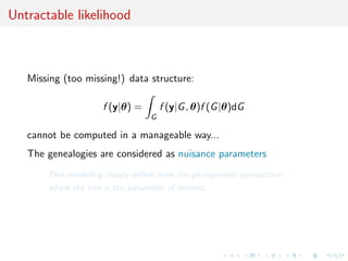
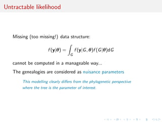


![ABC methodology
Bayesian setting: target is π(θ)f (x|θ)
When likelihood f (x|θ) not in closed form, likelihood-free rejection
technique:
Foundation
For an observation y ∼ f (y|θ), under the prior π(θ), if one keeps
jointly simulating
θ ∼ π(θ) , z ∼ f (z|θ ) ,
until the auxiliary variable z is equal to the observed value, z = y,
then the selected
θ ∼ π(θ|y)
[Rubin, 1984; Diggle & Gratton, 2984; Tavar´ et al., 1997]
e](https://image.slidesharecdn.com/abc-xian-120622072049-phpapp01/85/ABC-Xian-42-320.jpg)
![ABC methodology
Bayesian setting: target is π(θ)f (x|θ)
When likelihood f (x|θ) not in closed form, likelihood-free rejection
technique:
Foundation
For an observation y ∼ f (y|θ), under the prior π(θ), if one keeps
jointly simulating
θ ∼ π(θ) , z ∼ f (z|θ ) ,
until the auxiliary variable z is equal to the observed value, z = y,
then the selected
θ ∼ π(θ|y)
[Rubin, 1984; Diggle & Gratton, 2984; Tavar´ et al., 1997]
e](https://image.slidesharecdn.com/abc-xian-120622072049-phpapp01/85/ABC-Xian-43-320.jpg)
![ABC methodology
Bayesian setting: target is π(θ)f (x|θ)
When likelihood f (x|θ) not in closed form, likelihood-free rejection
technique:
Foundation
For an observation y ∼ f (y|θ), under the prior π(θ), if one keeps
jointly simulating
θ ∼ π(θ) , z ∼ f (z|θ ) ,
until the auxiliary variable z is equal to the observed value, z = y,
then the selected
θ ∼ π(θ|y)
[Rubin, 1984; Diggle & Gratton, 2984; Tavar´ et al., 1997]
e](https://image.slidesharecdn.com/abc-xian-120622072049-phpapp01/85/ABC-Xian-44-320.jpg)
![Why does it work?!
The proof is trivial:
f (θi ) ∝ π(θi )f (z|θi )Iy (z)
z∈D
∝ π(θi )f (y|θi )
= π(θi |y) .
[Accept–Reject 101]](https://image.slidesharecdn.com/abc-xian-120622072049-phpapp01/85/ABC-Xian-45-320.jpg)
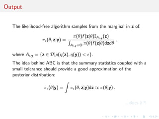
![A as A...pproximative
When y is a continuous random variable, strict equality z = y is
replaced with a tolerance zone
(y, z) ≤
where is a distance
Output distributed from
def
π(θ) Pθ { (y, z) < } ∝ π(θ| (y, z) < )
[Pritchard et al., 1999]](https://image.slidesharecdn.com/abc-xian-120622072049-phpapp01/85/ABC-Xian-46-320.jpg)
![A as A...pproximative
When y is a continuous random variable, strict equality z = y is
replaced with a tolerance zone
(y, z) ≤
where is a distance
Output distributed from
def
π(θ) Pθ { (y, z) < } ∝ π(θ| (y, z) < )
[Pritchard et al., 1999]](https://image.slidesharecdn.com/abc-xian-120622072049-phpapp01/85/ABC-Xian-47-320.jpg)


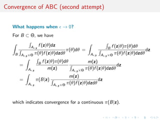
![Convergence of ABC (first attempt)
What happens when → 0?
If f (·|θ) is continuous in y , uniformly in θ [!], given an arbitrary
δ > 0, there exists 0 such that < 0 implies](https://image.slidesharecdn.com/abc-xian-120622072049-phpapp01/85/ABC-Xian-52-320.jpg)
![Convergence of ABC (first attempt)
What happens when → 0?
If f (·|θ) is continuous in y , uniformly in θ [!], given an arbitrary
δ > 0, there exists 0 such that < 0 implies
π(θ) f (z|θ)IA ,y (z) dz π(θ)f (y|θ)(1 δ)µ(B )
∈
A ,y ×Θ π(θ)f (z|θ)dzdθ Θ π(θ)f (y|θ)dθ(1 ± δ)µ(B )](https://image.slidesharecdn.com/abc-xian-120622072049-phpapp01/85/ABC-Xian-53-320.jpg)
![Convergence of ABC (first attempt)
What happens when → 0?
If f (·|θ) is continuous in y , uniformly in θ [!], given an arbitrary
δ > 0, there exists 0 such that < 0 implies
π(θ) f (z|θ)IA ,y (z) dz π(θ)f (y|θ)(1 δ)
XX )
µ(BX
∈
A ,y ×Θ π(θ)f (z|θ)dzdθ Θ π(θ)f (y|θ)dθ(1 ± δ) X
µ(B )
X
X](https://image.slidesharecdn.com/abc-xian-120622072049-phpapp01/85/ABC-Xian-54-320.jpg)
![Convergence of ABC (first attempt)
What happens when → 0?
If f (·|θ) is continuous in y , uniformly in θ [!], given an arbitrary
δ 0, there exists 0 such that 0 implies
π(θ) f (z|θ)IA ,y (z) dz π(θ)f (y|θ)(1 δ)
XX )
µ(BX
∈
A ,y ×Θ π(θ)f (z|θ)dzdθ Θ π(θ)f (y|θ)dθ(1 ± δ) X
µ(B )
X
X
[Proof extends to other continuous-in-0 kernels K ]](https://image.slidesharecdn.com/abc-xian-120622072049-phpapp01/85/ABC-Xian-55-320.jpg)


![MA example
MA(q) model
q
xt = t + ϑi t−i
i=1
Simple prior: uniform over the inverse [real and complex] roots in
q
Q(u) = 1 − ϑi u i
i=1
under the identifiability conditions](https://image.slidesharecdn.com/abc-xian-120622072049-phpapp01/85/ABC-Xian-67-320.jpg)


![ABC (simul’) advances
how approximative is ABC?
Simulating from the prior is often poor in efficiency
Either modify the proposal distribution on θ to increase the density
of x’s within the vicinity of y ...
[Marjoram et al, 2003; Bortot et al., 2007, Sisson et al., 2007]
...or by viewing the problem as a conditional density estimation
and by developing techniques to allow for larger
[Beaumont et al., 2002]
.....or even by including in the inferential framework [ABCµ ]
[Ratmann et al., 2009]](https://image.slidesharecdn.com/abc-xian-120622072049-phpapp01/85/ABC-Xian-74-320.jpg)
![ABC (simul’) advances
how approximative is ABC?
Simulating from the prior is often poor in efficiency
Either modify the proposal distribution on θ to increase the density
of x’s within the vicinity of y ...
[Marjoram et al, 2003; Bortot et al., 2007, Sisson et al., 2007]
...or by viewing the problem as a conditional density estimation
and by developing techniques to allow for larger
[Beaumont et al., 2002]
.....or even by including in the inferential framework [ABCµ ]
[Ratmann et al., 2009]](https://image.slidesharecdn.com/abc-xian-120622072049-phpapp01/85/ABC-Xian-75-320.jpg)
![ABC (simul’) advances
how approximative is ABC?
Simulating from the prior is often poor in efficiency
Either modify the proposal distribution on θ to increase the density
of x’s within the vicinity of y ...
[Marjoram et al, 2003; Bortot et al., 2007, Sisson et al., 2007]
...or by viewing the problem as a conditional density estimation
and by developing techniques to allow for larger
[Beaumont et al., 2002]
.....or even by including in the inferential framework [ABCµ ]
[Ratmann et al., 2009]](https://image.slidesharecdn.com/abc-xian-120622072049-phpapp01/85/ABC-Xian-76-320.jpg)
![ABC (simul’) advances
how approximative is ABC?
Simulating from the prior is often poor in efficiency
Either modify the proposal distribution on θ to increase the density
of x’s within the vicinity of y ...
[Marjoram et al, 2003; Bortot et al., 2007, Sisson et al., 2007]
...or by viewing the problem as a conditional density estimation
and by developing techniques to allow for larger
[Beaumont et al., 2002]
.....or even by including in the inferential framework [ABCµ ]
[Ratmann et al., 2009]](https://image.slidesharecdn.com/abc-xian-120622072049-phpapp01/85/ABC-Xian-77-320.jpg)
![ABC-NP
Better usage of [prior] simulations by
adjustement: instead of throwing away
θ such that ρ(η(z), η(y)) , replace
θ’s with locally regressed transforms
(use with BIC)
θ∗ = θ − {η(z) − η(y)}T β
ˆ [Csill´ry et al., TEE, 2010]
e
ˆ
where β is obtained by [NP] weighted least square regression on
(η(z) − η(y)) with weights
Kδ {ρ(η(z), η(y))}
[Beaumont et al., 2002, Genetics]](https://image.slidesharecdn.com/abc-xian-120622072049-phpapp01/85/ABC-Xian-78-320.jpg)
![ABC-NP (regression)
Also found in the subsequent literature, e.g. in Fearnhead-Prangle (2012) :
weight directly simulation by
Kδ {ρ(η(z(θ)), η(y))}
or
S
1
Kδ {ρ(η(zs (θ)), η(y))}
S
s=1
[consistent estimate of f (η|θ)]
Curse of dimensionality: poor estimate when d = dim(η) is large...](https://image.slidesharecdn.com/abc-xian-120622072049-phpapp01/85/ABC-Xian-79-320.jpg)
![ABC-NP (regression)
Also found in the subsequent literature, e.g. in Fearnhead-Prangle (2012) :
weight directly simulation by
Kδ {ρ(η(z(θ)), η(y))}
or
S
1
Kδ {ρ(η(zs (θ)), η(y))}
S
s=1
[consistent estimate of f (η|θ)]
Curse of dimensionality: poor estimate when d = dim(η) is large...](https://image.slidesharecdn.com/abc-xian-120622072049-phpapp01/85/ABC-Xian-80-320.jpg)
![ABC-NP (density estimation)
Use of the kernel weights
Kδ {ρ(η(z(θ)), η(y))}
leads to the NP estimate of the posterior expectation
i θi Kδ {ρ(η(z(θi )), η(y))}
i Kδ {ρ(η(z(θi )), η(y))}
[Blum, JASA, 2010]](https://image.slidesharecdn.com/abc-xian-120622072049-phpapp01/85/ABC-Xian-81-320.jpg)
![ABC-NP (density estimation)
Use of the kernel weights
Kδ {ρ(η(z(θ)), η(y))}
leads to the NP estimate of the posterior conditional density
˜
Kb (θi − θ)Kδ {ρ(η(z(θi )), η(y))}
i
i Kδ {ρ(η(z(θi )), η(y))}
[Blum, JASA, 2010]](https://image.slidesharecdn.com/abc-xian-120622072049-phpapp01/85/ABC-Xian-82-320.jpg)
![ABC-NP (density estimations)
Other versions incorporating regression adjustments
˜
Kb (θi∗ − θ)Kδ {ρ(η(z(θi )), η(y))}
i
i Kδ {ρ(η(z(θi )), η(y))}
In all cases, error
E[ˆ (θ|y)] − g (θ|y) = cb 2 + cδ 2 + OP (b 2 + δ 2 ) + OP (1/nδ d )
g
c
var(ˆ (θ|y)) =
g (1 + oP (1))
nbδ d](https://image.slidesharecdn.com/abc-xian-120622072049-phpapp01/85/ABC-Xian-83-320.jpg)
![ABC-NP (density estimations)
Other versions incorporating regression adjustments
˜
Kb (θi∗ − θ)Kδ {ρ(η(z(θi )), η(y))}
i
i Kδ {ρ(η(z(θi )), η(y))}
In all cases, error
E[ˆ (θ|y)] − g (θ|y) = cb 2 + cδ 2 + OP (b 2 + δ 2 ) + OP (1/nδ d )
g
c
var(ˆ (θ|y)) =
g (1 + oP (1))
nbδ d
[Blum, JASA, 2010]](https://image.slidesharecdn.com/abc-xian-120622072049-phpapp01/85/ABC-Xian-84-320.jpg)
![ABC-NP (density estimations)
Other versions incorporating regression adjustments
˜
Kb (θi∗ − θ)Kδ {ρ(η(z(θi )), η(y))}
i
i Kδ {ρ(η(z(θi )), η(y))}
In all cases, error
E[ˆ (θ|y)] − g (θ|y) = cb 2 + cδ 2 + OP (b 2 + δ 2 ) + OP (1/nδ d )
g
c
var(ˆ (θ|y)) =
g (1 + oP (1))
nbδ d
[standard NP calculations]](https://image.slidesharecdn.com/abc-xian-120622072049-phpapp01/85/ABC-Xian-85-320.jpg)
![ABC-NCH
Incorporating non-linearities and heterocedasticities:
σ (η(y))
ˆ
θ∗ = m(η(y)) + [θ − m(η(z))]
ˆ ˆ
σ (η(z))
ˆ
where
m(η) estimated by non-linear regression (e.g., neural network)
ˆ
σ (η) estimated by non-linear regression on residuals
ˆ
log{θi − m(ηi )}2 = log σ 2 (ηi ) + ξi
ˆ
[Blum Fran¸ois, 2009]
c](https://image.slidesharecdn.com/abc-xian-120622072049-phpapp01/85/ABC-Xian-86-320.jpg)
![ABC-NCH
Incorporating non-linearities and heterocedasticities:
σ (η(y))
ˆ
θ∗ = m(η(y)) + [θ − m(η(z))]
ˆ ˆ
σ (η(z))
ˆ
where
m(η) estimated by non-linear regression (e.g., neural network)
ˆ
σ (η) estimated by non-linear regression on residuals
ˆ
log{θi − m(ηi )}2 = log σ 2 (ηi ) + ξi
ˆ
[Blum Fran¸ois, 2009]
c](https://image.slidesharecdn.com/abc-xian-120622072049-phpapp01/85/ABC-Xian-87-320.jpg)
![ABC-NCH (2)
Why neural network?
fights curse of dimensionality
selects relevant summary statistics
provides automated dimension reduction
offers a model choice capability
improves upon multinomial logistic
[Blum Fran¸ois, 2009]
c](https://image.slidesharecdn.com/abc-xian-120622072049-phpapp01/85/ABC-Xian-88-320.jpg)
![ABC-NCH (2)
Why neural network?
fights curse of dimensionality
selects relevant summary statistics
provides automated dimension reduction
offers a model choice capability
improves upon multinomial logistic
[Blum Fran¸ois, 2009]
c](https://image.slidesharecdn.com/abc-xian-120622072049-phpapp01/85/ABC-Xian-89-320.jpg)
![ABC-MCMC
Markov chain (θ(t) ) created via the transition function
θ ∼ Kω (θ |θ(t) ) if x ∼ f (x|θ ) is such that x = y
π(θ )Kω (θ(t) |θ )
θ(t+1) = and u ∼ U(0, 1) ≤ π(θ(t) )Kω (θ |θ(t) )
,
(t)
θ otherwise,
has the posterior π(θ|y ) as stationary distribution
[Marjoram et al, 2003]](https://image.slidesharecdn.com/abc-xian-120622072049-phpapp01/85/ABC-Xian-90-320.jpg)
![ABC-MCMC
Markov chain (θ(t) ) created via the transition function
θ ∼ Kω (θ |θ(t) ) if x ∼ f (x|θ ) is such that x = y
π(θ )Kω (θ(t) |θ )
θ(t+1) = and u ∼ U(0, 1) ≤ π(θ(t) )Kω (θ |θ(t) )
,
(t)
θ otherwise,
has the posterior π(θ|y ) as stationary distribution
[Marjoram et al, 2003]](https://image.slidesharecdn.com/abc-xian-120622072049-phpapp01/85/ABC-Xian-91-320.jpg)
![ABC-MCMC (2)
Algorithm 2 Likelihood-free MCMC sampler
Use Algorithm 1 to get (θ(0) , z(0) )
for t = 1 to N do
Generate θ from Kω ·|θ(t−1) ,
Generate z from the likelihood f (·|θ ),
Generate u from U[0,1] ,
π(θ )Kω (θ(t−1) |θ )
if u ≤ I
π(θ(t−1) Kω (θ |θ(t−1) ) A ,y (z ) then
set (θ (t) , z(t) ) = (θ , z )
else
(θ(t) , z(t) )) = (θ(t−1) , z(t−1) ),
end if
end for](https://image.slidesharecdn.com/abc-xian-120622072049-phpapp01/85/ABC-Xian-92-320.jpg)


![A toy example
Case of
1 1
x ∼ N (θ, 1) + N (−θ, 1)
2 2
under prior θ ∼ N (0, 10)
ABC sampler
thetas=rnorm(N,sd=10)
zed=sample(c(1,-1),N,rep=TRUE)*thetas+rnorm(N,sd=1)
eps=quantile(abs(zed-x),.01)
abc=thetas[abs(zed-x)eps]](https://image.slidesharecdn.com/abc-xian-120622072049-phpapp01/85/ABC-Xian-96-320.jpg)
![A toy example
Case of
1 1
x ∼ N (θ, 1) + N (−θ, 1)
2 2
under prior θ ∼ N (0, 10)
ABC sampler
thetas=rnorm(N,sd=10)
zed=sample(c(1,-1),N,rep=TRUE)*thetas+rnorm(N,sd=1)
eps=quantile(abs(zed-x),.01)
abc=thetas[abs(zed-x)eps]](https://image.slidesharecdn.com/abc-xian-120622072049-phpapp01/85/ABC-Xian-97-320.jpg)
![A toy example
Case of
1 1
x ∼ N (θ, 1) + N (−θ, 1)
2 2
under prior θ ∼ N (0, 10)
ABC-MCMC sampler
metas=rep(0,N)
metas[1]=rnorm(1,sd=10)
zed[1]=x
for (t in 2:N){
metas[t]=rnorm(1,mean=metas[t-1],sd=5)
zed[t]=rnorm(1,mean=(1-2*(runif(1).5))*metas[t],sd=1)
if ((abs(zed[t]-x)eps)||(runif(1)dnorm(metas[t],sd=10)/dnorm(metas[t-1],sd=10))){
metas[t]=metas[t-1]
zed[t]=zed[t-1]}
}](https://image.slidesharecdn.com/abc-xian-120622072049-phpapp01/85/ABC-Xian-98-320.jpg)


![ABC-PMC
Use of a transition kernel as in population Monte Carlo with
manageable IS correction
Generate a sample at iteration t by
N
(t−1) (t−1)
πt (θ(t) ) ∝
ˆ ωj Kt (θ(t) |θj )
j=1
modulo acceptance of the associated xt , and use an importance
(t)
weight associated with an accepted simulation θi
(t) (t) (t)
ωi ∝ π(θi ) πt (θi ) .
ˆ
c Still likelihood free
[Beaumont et al., 2009]](https://image.slidesharecdn.com/abc-xian-120622072049-phpapp01/85/ABC-Xian-105-320.jpg)

![Sequential Monte Carlo
SMC is a simulation technique to approximate a sequence of
related probability distributions πn with π0 “easy” and πT as
target.
Iterated IS as PMC: particles moved from time n to time n via
kernel Kn and use of a sequence of extended targets πn˜
n
πn (z0:n ) = πn (zn )
˜ Lj (zj+1 , zj )
j=0
where the Lj ’s are backward Markov kernels [check that πn (zn ) is a
marginal]
[Del Moral, Doucet Jasra, Series B, 2006]](https://image.slidesharecdn.com/abc-xian-120622072049-phpapp01/85/ABC-Xian-107-320.jpg)
![Sequential Monte Carlo (2)
Algorithm 3 SMC sampler
(0)
sample zi ∼ γ0 (x) (i = 1, . . . , N)
(0) (0) (0)
compute weights wi = π0 (zi )/γ0 (zi )
for t = 1 to N do
if ESS(w (t−1) ) NT then
resample N particles z (t−1) and set weights to 1
end if
(t−1) (t−1)
generate zi ∼ Kt (zi , ·) and set weights to
(t) (t) (t−1)
(t) (t−1) πt (zi ))Lt−1 (zi ), zi ))
wi = wi−1 (t−1) (t−1) (t)
πt−1 (zi ))Kt (zi ), zi ))
end for
[Del Moral, Doucet Jasra, Series B, 2006]](https://image.slidesharecdn.com/abc-xian-120622072049-phpapp01/85/ABC-Xian-108-320.jpg)
![ABC-SMC
[Del Moral, Doucet Jasra, 2009]
True derivation of an SMC-ABC algorithm
Use of a kernel Kn associated with target π n and derivation of the
backward kernel
π n (z )Kn (z , z)
Ln−1 (z, z ) =
πn (z)
Update of the weights
M m
m=1 IA n
(xin )
win ∝ wi(n−1) M m
(xi(n−1) )
m=1 IA n−1
m
when xin ∼ K (xi(n−1) , ·)](https://image.slidesharecdn.com/abc-xian-120622072049-phpapp01/85/ABC-Xian-109-320.jpg)
![ABC-SMCM
Modification: Makes M repeated simulations of the pseudo-data z
given the parameter, rather than using a single [M = 1] simulation,
leading to weight that is proportional to the number of accepted
zi s
M
1
ω(θ) = Iρ(η(y),η(zi ))
M
i=1
[limit in M means exact simulation from (tempered) target]](https://image.slidesharecdn.com/abc-xian-120622072049-phpapp01/85/ABC-Xian-110-320.jpg)
![Properties of ABC-SMC
The ABC-SMC method properly uses a backward kernel L(z, z ) to
simplify the importance weight and to remove the dependence on
the unknown likelihood from this weight. Update of importance
weights is reduced to the ratio of the proportions of surviving
particles
Major assumption: the forward kernel K is supposed to be invariant
against the true target [tempered version of the true posterior]
Adaptivity in ABC-SMC algorithm only found in on-line
construction of the thresholds t , slowly enough to keep a large
number of accepted transitions](https://image.slidesharecdn.com/abc-xian-120622072049-phpapp01/85/ABC-Xian-111-320.jpg)
![Properties of ABC-SMC
The ABC-SMC method properly uses a backward kernel L(z, z ) to
simplify the importance weight and to remove the dependence on
the unknown likelihood from this weight. Update of importance
weights is reduced to the ratio of the proportions of surviving
particles
Major assumption: the forward kernel K is supposed to be invariant
against the true target [tempered version of the true posterior]
Adaptivity in ABC-SMC algorithm only found in on-line
construction of the thresholds t , slowly enough to keep a large
number of accepted transitions](https://image.slidesharecdn.com/abc-xian-120622072049-phpapp01/85/ABC-Xian-112-320.jpg)
![A mixture example (1)
Toy model of Sisson et al. (2007): if
θ ∼ U(−10, 10) , x|θ ∼ 0.5 N (θ, 1) + 0.5 N (θ, 1/100) ,
then the posterior distribution associated with y = 0 is the normal
mixture
θ|y = 0 ∼ 0.5 N (0, 1) + 0.5 N (0, 1/100)
restricted to [−10, 10].
Furthermore, true target available as
π(θ||x| ) ∝ Φ( −θ)−Φ(− −θ)+Φ(10( −θ))−Φ(−10( +θ)) .](https://image.slidesharecdn.com/abc-xian-120622072049-phpapp01/85/ABC-Xian-113-320.jpg)

![Yet another ABC-PRC
Another version of ABC-PRC called PRC-ABC with a proposal
distribution Mt , S replications of the pseudo-data, and a PRC step:
PRC-ABC Algorithm
(t−1) (t−1)
1. Select θ at random from the θi ’s with probabilities ωi
(t) iid (t−1)
2. Generate θi ∼ Kt , x1 , . . . , xS ∼ f (x|θi ), set
(t) (t)
ωi = Kt {η(xs ) − η(y)} Kt (θi ) ,
s
(t)
and accept with probability p (i) = ωi /ct,N
(t) (t)
3. Set ωi ∝ ωi /p (i) (1 ≤ i ≤ N)
[Peters, Sisson Fan, Stat Computing, 2012]](https://image.slidesharecdn.com/abc-xian-120622072049-phpapp01/85/ABC-Xian-115-320.jpg)


![ABCµ
Idea Infer about the error as well:
Use of a joint density
f (θ, |y) ∝ ξ( |y, θ) × πθ (θ) × π ( )
where y is the data, and ξ( |y, θ) is the prior predictive density of
ρ(η(z), η(y)) given θ and y when z ∼ f (z|θ)
Warning! Replacement of ξ( |y, θ) with a non-parametric kernel
approximation.
[Ratmann, Andrieu, Wiuf and Richardson, 2009, PNAS]](https://image.slidesharecdn.com/abc-xian-120622072049-phpapp01/85/ABC-Xian-120-320.jpg)
![ABCµ
Idea Infer about the error as well:
Use of a joint density
f (θ, |y) ∝ ξ( |y, θ) × πθ (θ) × π ( )
where y is the data, and ξ( |y, θ) is the prior predictive density of
ρ(η(z), η(y)) given θ and y when z ∼ f (z|θ)
Warning! Replacement of ξ( |y, θ) with a non-parametric kernel
approximation.
[Ratmann, Andrieu, Wiuf and Richardson, 2009, PNAS]](https://image.slidesharecdn.com/abc-xian-120622072049-phpapp01/85/ABC-Xian-121-320.jpg)
![ABCµ
Idea Infer about the error as well:
Use of a joint density
f (θ, |y) ∝ ξ( |y, θ) × πθ (θ) × π ( )
where y is the data, and ξ( |y, θ) is the prior predictive density of
ρ(η(z), η(y)) given θ and y when z ∼ f (z|θ)
Warning! Replacement of ξ( |y, θ) with a non-parametric kernel
approximation.
[Ratmann, Andrieu, Wiuf and Richardson, 2009, PNAS]](https://image.slidesharecdn.com/abc-xian-120622072049-phpapp01/85/ABC-Xian-122-320.jpg)
![ABCµ details
Multidimensional distances ρk (k = 1, . . . , K ) and errors
k = ρk (ηk (z), ηk (y)), with
ˆ 1
k ∼ ξk ( |y, θ) ≈ ξk ( |y, θ) = K [{ k −ρk (ηk (zb ), ηk (y))}/hk ]
Bhk
b
ˆ
then used in replacing ξ( |y, θ) with mink ξk ( |y, θ)
ABCµ involves acceptance probability
ˆ
π(θ , ) q(θ , θ)q( , ) mink ξk ( |y, θ )
ˆ
π(θ, ) q(θ, θ )q( , ) mink ξk ( |y, θ)](https://image.slidesharecdn.com/abc-xian-120622072049-phpapp01/85/ABC-Xian-123-320.jpg)
![ABCµ details
Multidimensional distances ρk (k = 1, . . . , K ) and errors
k = ρk (ηk (z), ηk (y)), with
ˆ 1
k ∼ ξk ( |y, θ) ≈ ξk ( |y, θ) = K [{ k −ρk (ηk (zb ), ηk (y))}/hk ]
Bhk
b
ˆ
then used in replacing ξ( |y, θ) with mink ξk ( |y, θ)
ABCµ involves acceptance probability
ˆ
π(θ , ) q(θ , θ)q( , ) mink ξk ( |y, θ )
ˆ
π(θ, ) q(θ, θ )q( , ) mink ξk ( |y, θ)](https://image.slidesharecdn.com/abc-xian-120622072049-phpapp01/85/ABC-Xian-124-320.jpg)
![ABCµ multiple errors
[ c Ratmann et al., PNAS, 2009]](https://image.slidesharecdn.com/abc-xian-120622072049-phpapp01/85/ABC-Xian-125-320.jpg)
![ABCµ for model choice
[ c Ratmann et al., PNAS, 2009]](https://image.slidesharecdn.com/abc-xian-120622072049-phpapp01/85/ABC-Xian-126-320.jpg)
![Questions about ABCµ
For each model under comparison, marginal posterior on used to
assess the fit of the model (HPD includes 0 or not).
Is the data informative about ? [Identifiability]
How much does the prior π( ) impact the comparison?
How is using both ξ( |x0 , θ) and π ( ) compatible with a
standard probability model? [remindful of Wilkinson’s eABC ]
Where is the penalisation for complexity in the model
comparison?
[X, Mengersen Chen, 2010, PNAS]](https://image.slidesharecdn.com/abc-xian-120622072049-phpapp01/85/ABC-Xian-127-320.jpg)
![Questions about ABCµ
For each model under comparison, marginal posterior on used to
assess the fit of the model (HPD includes 0 or not).
Is the data informative about ? [Identifiability]
How much does the prior π( ) impact the comparison?
How is using both ξ( |x0 , θ) and π ( ) compatible with a
standard probability model? [remindful of Wilkinson’s eABC ]
Where is the penalisation for complexity in the model
comparison?
[X, Mengersen Chen, 2010, PNAS]](https://image.slidesharecdn.com/abc-xian-120622072049-phpapp01/85/ABC-Xian-128-320.jpg)
![Wilkinson’s exact BC (not exactly!)
ABC approximation error (i.e. non-zero tolerance) replaced with
exact simulation from a controlled approximation to the target,
convolution of true posterior with kernel function
π(θ)f (z|θ)K (y − z)
π (θ, z|y) = ,
π(θ)f (z|θ)K (y − z)dzdθ
with K kernel parameterised by bandwidth .
[Wilkinson, 2008]
Theorem
The ABC algorithm based on the assumption of a randomised
observation y = y + ξ, ξ ∼ K , and an acceptance probability of
˜
K (y − z)/M
gives draws from the posterior distribution π(θ|y).](https://image.slidesharecdn.com/abc-xian-120622072049-phpapp01/85/ABC-Xian-129-320.jpg)
![Wilkinson’s exact BC (not exactly!)
ABC approximation error (i.e. non-zero tolerance) replaced with
exact simulation from a controlled approximation to the target,
convolution of true posterior with kernel function
π(θ)f (z|θ)K (y − z)
π (θ, z|y) = ,
π(θ)f (z|θ)K (y − z)dzdθ
with K kernel parameterised by bandwidth .
[Wilkinson, 2008]
Theorem
The ABC algorithm based on the assumption of a randomised
observation y = y + ξ, ξ ∼ K , and an acceptance probability of
˜
K (y − z)/M
gives draws from the posterior distribution π(θ|y).](https://image.slidesharecdn.com/abc-xian-120622072049-phpapp01/85/ABC-Xian-130-320.jpg)
![How exact a BC?
“Using to represent measurement error is
straightforward, whereas using to model the model
discrepancy is harder to conceptualize and not as
commonly used”
[Richard Wilkinson, 2008]](https://image.slidesharecdn.com/abc-xian-120622072049-phpapp01/85/ABC-Xian-131-320.jpg)
![How exact a BC?
Pros
Pseudo-data from true model and observed data from noisy
model
Interesting perspective in that outcome is completely
controlled
Link with ABCµ and assuming y is observed with a
measurement error with density K
Relates to the theory of model approximation
[Kennedy O’Hagan, 2001]
Cons
Requires K to be bounded by M
True approximation error never assessed
Requires a modification of the standard ABC algorithm](https://image.slidesharecdn.com/abc-xian-120622072049-phpapp01/85/ABC-Xian-132-320.jpg)
![ABC for HMMs
Specific case of a hidden Markov model
Xt+1 ∼ Qθ (Xt , ·)
Yt+1 ∼ gθ (·|xt )
0
where only y1:n is observed.
[Dean, Singh, Jasra, Peters, 2011]
Use of specific constraints, adapted to the Markov structure:
0 0
y1 ∈ B(y1 , ) × · · · × yn ∈ B(yn , )](https://image.slidesharecdn.com/abc-xian-120622072049-phpapp01/85/ABC-Xian-133-320.jpg)
![ABC for HMMs
Specific case of a hidden Markov model
Xt+1 ∼ Qθ (Xt , ·)
Yt+1 ∼ gθ (·|xt )
0
where only y1:n is observed.
[Dean, Singh, Jasra, Peters, 2011]
Use of specific constraints, adapted to the Markov structure:
0 0
y1 ∈ B(y1 , ) × · · · × yn ∈ B(yn , )](https://image.slidesharecdn.com/abc-xian-120622072049-phpapp01/85/ABC-Xian-134-320.jpg)
![ABC-MLE for HMMs
ABC-MLE defined by
ˆ 0 0
θn = arg max Pθ Y1 ∈ B(y1 , ), . . . , Yn ∈ B(yn , )
θ
Exact MLE for the likelihood same basis as Wilkinson!
0
pθ (y1 , . . . , yn )
corresponding to the perturbed process
(xt , yt + zt )1≤t≤n zt ∼ U(B(0, 1)
[Dean, Singh, Jasra, Peters, 2011]](https://image.slidesharecdn.com/abc-xian-120622072049-phpapp01/85/ABC-Xian-135-320.jpg)
![ABC-MLE for HMMs
ABC-MLE defined by
ˆ 0 0
θn = arg max Pθ Y1 ∈ B(y1 , ), . . . , Yn ∈ B(yn , )
θ
Exact MLE for the likelihood same basis as Wilkinson!
0
pθ (y1 , . . . , yn )
corresponding to the perturbed process
(xt , yt + zt )1≤t≤n zt ∼ U(B(0, 1)
[Dean, Singh, Jasra, Peters, 2011]](https://image.slidesharecdn.com/abc-xian-120622072049-phpapp01/85/ABC-Xian-136-320.jpg)
![ABC-MLE is biased
ABC-MLE is asymptotically (in n) biased with target
l (θ) = Eθ∗ [log pθ (Y1 |Y−∞:0 )]
but ABC-MLE converges to true value in the sense
l n (θn ) → l (θ)
for all sequences (θn ) converging to θ and n](https://image.slidesharecdn.com/abc-xian-120622072049-phpapp01/85/ABC-Xian-137-320.jpg)
![ABC-MLE is biased
ABC-MLE is asymptotically (in n) biased with target
l (θ) = Eθ∗ [log pθ (Y1 |Y−∞:0 )]
but ABC-MLE converges to true value in the sense
l n (θn ) → l (θ)
for all sequences (θn ) converging to θ and n](https://image.slidesharecdn.com/abc-xian-120622072049-phpapp01/85/ABC-Xian-138-320.jpg)
![Noisy ABC-MLE
Idea: Modify instead the data from the start
0
(y1 + ζ1 , . . . , yn + ζn )
[ see Fearnhead-Prangle ]
noisy ABC-MLE estimate
0 0
arg max Pθ Y1 ∈ B(y1 + ζ1 , ), . . . , Yn ∈ B(yn + ζn , )
θ
[Dean, Singh, Jasra, Peters, 2011]](https://image.slidesharecdn.com/abc-xian-120622072049-phpapp01/85/ABC-Xian-139-320.jpg)
![Consistent noisy ABC-MLE
Degrading the data improves the estimation performances:
Noisy ABC-MLE is asymptotically (in n) consistent
under further assumptions, the noisy ABC-MLE is
asymptotically normal
increase in variance of order −2
likely degradation in precision or computing time due to the
lack of summary statistic [curse of dimensionality]](https://image.slidesharecdn.com/abc-xian-120622072049-phpapp01/85/ABC-Xian-140-320.jpg)
![SMC for ABC likelihood
Algorithm 4 SMC ABC for HMMs
Given θ
for k = 1, . . . , n do
1 1 N N
generate proposals (xk , yk ), . . . , (xk , yk ) from the model
weigh each proposal with ωk l =I l
B(yk + ζk , ) (yk )
0
l
renormalise the weights and sample the xk ’s accordingly
end for
approximate the likelihood by
n N
l
ωk N
k=1 l=1
[Jasra, Singh, Martin, McCoy, 2010]](https://image.slidesharecdn.com/abc-xian-120622072049-phpapp01/85/ABC-Xian-141-320.jpg)
![Which summary?
Fundamental difficulty of the choice of the summary statistic when
there is no non-trivial sufficient statistics [except when done by the
experimenters in the field]
Starting from a large collection of summary statistics is available,
Joyce and Marjoram (2008) consider the sequential inclusion into
the ABC target, with a stopping rule based on a likelihood ratio
test
Not taking into account the sequential nature of the tests
Depends on parameterisation
Order of inclusion matters](https://image.slidesharecdn.com/abc-xian-120622072049-phpapp01/85/ABC-Xian-142-320.jpg)
![Which summary?
Fundamental difficulty of the choice of the summary statistic when
there is no non-trivial sufficient statistics [except when done by the
experimenters in the field]
Starting from a large collection of summary statistics is available,
Joyce and Marjoram (2008) consider the sequential inclusion into
the ABC target, with a stopping rule based on a likelihood ratio
test
Not taking into account the sequential nature of the tests
Depends on parameterisation
Order of inclusion matters](https://image.slidesharecdn.com/abc-xian-120622072049-phpapp01/85/ABC-Xian-143-320.jpg)
![Which summary?
Fundamental difficulty of the choice of the summary statistic when
there is no non-trivial sufficient statistics [except when done by the
experimenters in the field]
Starting from a large collection of summary statistics is available,
Joyce and Marjoram (2008) consider the sequential inclusion into
the ABC target, with a stopping rule based on a likelihood ratio
test
Not taking into account the sequential nature of the tests
Depends on parameterisation
Order of inclusion matters](https://image.slidesharecdn.com/abc-xian-120622072049-phpapp01/85/ABC-Xian-144-320.jpg)
![Semi-automatic ABC
Fearnhead and Prangle (2010) study ABC and the selection of the
summary statistic in close proximity to Wilkinson’s proposal
ABC then considered from a purely inferential viewpoint and
calibrated for estimation purposes
Use of a randomised (or ‘noisy’) version of the summary statistics
η (y) = η(y) + τ
˜
Derivation of a well-calibrated version of ABC, i.e. an algorithm
that gives proper predictions for the distribution associated with
this randomised summary statistic [calibration constraint: ABC
approximation with same posterior mean as the true randomised
posterior]](https://image.slidesharecdn.com/abc-xian-120622072049-phpapp01/85/ABC-Xian-145-320.jpg)
![Semi-automatic ABC
Fearnhead and Prangle (2010) study ABC and the selection of the
summary statistic in close proximity to Wilkinson’s proposal
ABC then considered from a purely inferential viewpoint and
calibrated for estimation purposes
Use of a randomised (or ‘noisy’) version of the summary statistics
η (y) = η(y) + τ
˜
Derivation of a well-calibrated version of ABC, i.e. an algorithm
that gives proper predictions for the distribution associated with
this randomised summary statistic [calibration constraint: ABC
approximation with same posterior mean as the true randomised
posterior]](https://image.slidesharecdn.com/abc-xian-120622072049-phpapp01/85/ABC-Xian-146-320.jpg)
![Summary statistics
Optimality of the posterior expectation E[θ|y] of the
parameter of interest as summary statistics η(y)!
Use of the standard quadratic loss function
(θ − θ0 )T A(θ − θ0 ) .](https://image.slidesharecdn.com/abc-xian-120622072049-phpapp01/85/ABC-Xian-147-320.jpg)
![Summary statistics
Optimality of the posterior expectation E[θ|y] of the
parameter of interest as summary statistics η(y)!
Use of the standard quadratic loss function
(θ − θ0 )T A(θ − θ0 ) .](https://image.slidesharecdn.com/abc-xian-120622072049-phpapp01/85/ABC-Xian-148-320.jpg)
![Details on Fearnhead and Prangle (FP) ABC
Use of a summary statistic S(·), an importance proposal g (·), a
kernel K (·) ≤ 1 and a bandwidth h 0 such that
(θ, ysim ) ∼ g (θ)f (ysim |θ)
is accepted with probability (hence the bound)
K [{S(ysim ) − sobs }/h]
and the corresponding importance weight defined by
π(θ) g (θ)
[Fearnhead Prangle, 2012]](https://image.slidesharecdn.com/abc-xian-120622072049-phpapp01/85/ABC-Xian-149-320.jpg)
![Errors, errors, and errors
Three levels of approximation
π(θ|yobs ) by π(θ|sobs ) loss of information
[ignored]
π(θ|sobs ) by
π(s)K [{s − sobs }/h]π(θ|s) ds
πABC (θ|sobs ) =
π(s)K [{s − sobs }/h] ds
noisy observations
πABC (θ|sobs ) by importance Monte Carlo based on N
simulations, represented by var(a(θ)|sobs )/Nacc [expected
number of acceptances]
[M. Twain/B. Disraeli]](https://image.slidesharecdn.com/abc-xian-120622072049-phpapp01/85/ABC-Xian-150-320.jpg)
![Average acceptance asymptotics
For the average acceptance probability/approximate likelihood
p(θ|sobs ) = f (ysim |θ) K [{S(ysim ) − sobs }/h] dysim ,
overall acceptance probability
p(sobs ) = p(θ|sobs ) π(θ) dθ = π(sobs )hd + o(hd )
[FP, Lemma 1]](https://image.slidesharecdn.com/abc-xian-120622072049-phpapp01/85/ABC-Xian-151-320.jpg)
![Optimal importance proposal
Best choice of importance proposal in terms of effective sample size
g (θ|sobs ) ∝ π(θ)p(θ|sobs )1/2
[Not particularly useful in practice]
note that p(θ|sobs ) is an approximate likelihood
reminiscent of parallel tempering
could be approximately achieved by attrition of half of the
data](https://image.slidesharecdn.com/abc-xian-120622072049-phpapp01/85/ABC-Xian-152-320.jpg)
![Optimal importance proposal
Best choice of importance proposal in terms of effective sample size
g (θ|sobs ) ∝ π(θ)p(θ|sobs )1/2
[Not particularly useful in practice]
note that p(θ|sobs ) is an approximate likelihood
reminiscent of parallel tempering
could be approximately achieved by attrition of half of the
data](https://image.slidesharecdn.com/abc-xian-120622072049-phpapp01/85/ABC-Xian-153-320.jpg)
![Calibration of h
“This result gives insight into how S(·) and h affect the Monte
Carlo error. To minimize Monte Carlo error, we need hd to be not
too small. Thus ideally we want S(·) to be a low dimensional
summary of the data that is sufficiently informative about θ that
π(θ|sobs ) is close, in some sense, to π(θ|yobs )” (FP, p.5)
turns h into an absolute value while it should be
context-dependent and user-calibrated
only addresses one term in the approximation error and
acceptance probability (“curse of dimensionality”)
h large prevents πABC (θ|sobs ) to be close to π(θ|sobs )
d small prevents π(θ|sobs ) to be close to π(θ|yobs ) (“curse of
[dis]information”)](https://image.slidesharecdn.com/abc-xian-120622072049-phpapp01/85/ABC-Xian-154-320.jpg)


![Calibrated ABC
Theorem (FP)
Noisy ABC, where
sobs = S(yobs ) + h , ∼ K (·)
is calibrated
[Wilkinson, 2008]
no condition on h!!](https://image.slidesharecdn.com/abc-xian-120622072049-phpapp01/85/ABC-Xian-157-320.jpg)

![More questions about calibrated ABC
“Calibration is not universally accepted by Bayesians. It is even more
questionable here as we care how statements we make relate to the
real world, not to a mathematically defined posterior.” R. Wilkinson
Same reluctance about the prior being calibrated
Property depending on prior, likelihood, and summary
Calibration is a frequentist property (almost a p-value!)
More sensible to account for the simulator’s imperfections
than using noisy-ABC against a meaningless based measure
[Wilkinson, 2012]](https://image.slidesharecdn.com/abc-xian-120622072049-phpapp01/85/ABC-Xian-159-320.jpg)
![Converging ABC
Theorem (FP)
For noisy ABC, the expected noisy-ABC log-likelihood,
E {log[p(θ|sobs )]} = log[p(θ|S(yobs ) + )]π(yobs |θ0 )K ( )dyobs d ,
has its maximum at θ = θ0 .
True for any choice of summary statistic? even ancilary statistics?!
[Imposes at least identifiability...]
Relevant in asymptotia and not for the data](https://image.slidesharecdn.com/abc-xian-120622072049-phpapp01/85/ABC-Xian-160-320.jpg)
![Converging ABC
Corollary
For noisy ABC, the ABC posterior converges onto a point mass on
the true parameter value as m → ∞.
For standard ABC, not always the case (unless h goes to zero).
Strength of regularity conditions (c1) and (c2) in Bernardo
Smith, 1994?
[out-of-reach constraints on likelihood and posterior]
Again, there must be conditions imposed upon summary
statistics...](https://image.slidesharecdn.com/abc-xian-120622072049-phpapp01/85/ABC-Xian-161-320.jpg)
![Loss motivated statistic
Under quadratic loss function,
Theorem (FP)
ˆ
(i) The minimal posterior error E[L(θ, θ)|yobs ] occurs when
ˆ = E(θ|yobs ) (!)
θ
(ii) When h → 0, EABC (θ|sobs ) converges to E(θ|yobs )
ˆ
(iii) If S(yobs ) = E[θ|yobs ] then for θ = EABC [θ|sobs ]
ˆ
E[L(θ, θ)|yobs ] = trace(AΣ) + h2 xT AxK (x)dx + o(h2 ).
measure-theoretic difficulties?
dependence of sobs on h makes me uncomfortable inherent to noisy
ABC
Relevant for choice of K ?](https://image.slidesharecdn.com/abc-xian-120622072049-phpapp01/85/ABC-Xian-162-320.jpg)
![Optimal summary statistic
“We take a different approach, and weaken the requirement for
πABC to be a good approximation to π(θ|yobs ). We argue for πABC
to be a good approximation solely in terms of the accuracy of
certain estimates of the parameters.” (FP, p.5)
From this result, FP
derive their choice of summary statistic,
S(y) = E(θ|y)
[almost sufficient]
suggest
h = O(N −1/(2+d) ) and h = O(N −1/(4+d) )
as optimal bandwidths for noisy and standard ABC.](https://image.slidesharecdn.com/abc-xian-120622072049-phpapp01/85/ABC-Xian-163-320.jpg)
![Optimal summary statistic
“We take a different approach, and weaken the requirement for
πABC to be a good approximation to π(θ|yobs ). We argue for πABC
to be a good approximation solely in terms of the accuracy of
certain estimates of the parameters.” (FP, p.5)
From this result, FP
derive their choice of summary statistic,
S(y) = E(θ|y)
[wow! EABC [θ|S(yobs )] = E[θ|yobs ]]
suggest
h = O(N −1/(2+d) ) and h = O(N −1/(4+d) )
as optimal bandwidths for noisy and standard ABC.](https://image.slidesharecdn.com/abc-xian-120622072049-phpapp01/85/ABC-Xian-164-320.jpg)


![Approximating the summary statistic
As Beaumont et al. (2002) and Blum and Fran¸ois (2010), FP
c
use a linear regression to approximate E(θ|yobs ):
(i)
θi = β0 + β (i) f (yobs ) + i
with f made of standard transforms
[Further justifications?]](https://image.slidesharecdn.com/abc-xian-120622072049-phpapp01/85/ABC-Xian-167-320.jpg)
![[my]questions about semi-automatic ABC
dependence on h and S(·) in the early stage
reduction of Bayesian inference to point estimation
approximation error in step (i) not accounted for
not parameterisation invariant
practice shows that proper approximation to genuine posterior
distributions stems from using a (much) larger number of
summary statistics than the dimension of the parameter
the validity of the approximation to the optimal summary
statistic depends on the quality of the pilot run
important inferential issues like model choice are not covered
by this approach.
[Robert, 2012]](https://image.slidesharecdn.com/abc-xian-120622072049-phpapp01/85/ABC-Xian-168-320.jpg)
![More about semi-automatic ABC
[End of section derived from comments on Read Paper, just appeared]
“The apparently arbitrary nature of the choice of summary statistics
has always been perceived as the Achilles heel of ABC.” M.
Beaumont
“Curse of dimensionality” linked with the increase of the
dimension of the summary statistic
Connection with principal component analysis
[Itan et al., 2010]
Connection with partial least squares
[Wegman et al., 2009]
Beaumont et al. (2002) postprocessed output is used as input
by FP to run a second ABC](https://image.slidesharecdn.com/abc-xian-120622072049-phpapp01/85/ABC-Xian-169-320.jpg)
![More about semi-automatic ABC
[End of section derived from comments on Read Paper, just appeared]
“The apparently arbitrary nature of the choice of summary statistics
has always been perceived as the Achilles heel of ABC.” M.
Beaumont
“Curse of dimensionality” linked with the increase of the
dimension of the summary statistic
Connection with principal component analysis
[Itan et al., 2010]
Connection with partial least squares
[Wegman et al., 2009]
Beaumont et al. (2002) postprocessed output is used as input
by FP to run a second ABC](https://image.slidesharecdn.com/abc-xian-120622072049-phpapp01/85/ABC-Xian-170-320.jpg)
![Wood’s alternative
Instead of a non-parametric kernel approximation to the likelihood
1
K {η(yr ) − η(yobs )}
R r
Wood (2010) suggests a normal approximation
η(y(θ)) ∼ Nd (µθ , Σθ )
whose parameters can be approximated based on the R simulations
(for each value of θ).
Parametric versus non-parametric rate [Uh?!]
Automatic weighting of components of η(·) through Σθ
Dependence on normality assumption (pseudo-likelihood?)
[Cornebise, Girolami Kosmidis, 2012]](https://image.slidesharecdn.com/abc-xian-120622072049-phpapp01/85/ABC-Xian-171-320.jpg)
![Wood’s alternative
Instead of a non-parametric kernel approximation to the likelihood
1
K {η(yr ) − η(yobs )}
R r
Wood (2010) suggests a normal approximation
η(y(θ)) ∼ Nd (µθ , Σθ )
whose parameters can be approximated based on the R simulations
(for each value of θ).
Parametric versus non-parametric rate [Uh?!]
Automatic weighting of components of η(·) through Σθ
Dependence on normality assumption (pseudo-likelihood?)
[Cornebise, Girolami Kosmidis, 2012]](https://image.slidesharecdn.com/abc-xian-120622072049-phpapp01/85/ABC-Xian-172-320.jpg)
![Reinterpretation and extensions
Reinterpretation of ABC output as joint simulation from
π (x, y |θ) = f (x|θ)¯Y |X (y |x)
¯ π
where
πY |X (y |x) = K (y − x)
¯
Reinterpretation of noisy ABC
if y |y obs ∼ πY |X (·|y obs ), then marginally
¯ ¯
y ∼ πY |θ (·|θ0 )
¯ ¯
c Explain for the consistency of Bayesian inference based on y and π
¯ ¯
[Lee, Andrieu Doucet, 2012]](https://image.slidesharecdn.com/abc-xian-120622072049-phpapp01/85/ABC-Xian-173-320.jpg)
![Reinterpretation and extensions
Reinterpretation of ABC output as joint simulation from
π (x, y |θ) = f (x|θ)¯Y |X (y |x)
¯ π
where
πY |X (y |x) = K (y − x)
¯
Reinterpretation of noisy ABC
if y |y obs ∼ πY |X (·|y obs ), then marginally
¯ ¯
y ∼ πY |θ (·|θ0 )
¯ ¯
c Explain for the consistency of Bayesian inference based on y and π
¯ ¯
[Lee, Andrieu Doucet, 2012]](https://image.slidesharecdn.com/abc-xian-120622072049-phpapp01/85/ABC-Xian-174-320.jpg)
![ABC for Markov chains
Rewriting the posterior as
π(θ)1−n π(θ|x1 ) π(θ|xt−1 , xt )
where π(θ|xt−1 , xt ) ∝ f (xt |xt−1 , θ)π(θ)
Allows for a stepwise ABC, replacing each π(θ|xt−1 , xt ) by an
ABC approximation
Similarity with FP’s multiple sources of data (and also with
Dean et al., 2011 )
[White et al., 2010, 2012]](https://image.slidesharecdn.com/abc-xian-120622072049-phpapp01/85/ABC-Xian-175-320.jpg)
![ABC for Markov chains
Rewriting the posterior as
π(θ)1−n π(θ|x1 ) π(θ|xt−1 , xt )
where π(θ|xt−1 , xt ) ∝ f (xt |xt−1 , θ)π(θ)
Allows for a stepwise ABC, replacing each π(θ|xt−1 , xt ) by an
ABC approximation
Similarity with FP’s multiple sources of data (and also with
Dean et al., 2011 )
[White et al., 2010, 2012]](https://image.slidesharecdn.com/abc-xian-120622072049-phpapp01/85/ABC-Xian-176-320.jpg)
![Back to sufficiency
Difference between regular sufficiency, equivalent to
π(θ|y) = π(θ|η(y))
for all θ’s and all priors π, and
marginal sufficiency, stated as
π(µ(θ)|y) = π(µ(θ)|η(y))
for all θ’s, the given prior π and a subvector µ(θ)
[Basu, 1977]
Relates to F P’s main result, but could event be reduced to
conditional sufficiency
π(µ(θ)|yobs ) = π(µ(θ)|η(yobs ))
(if feasible at all...)
[Dawson, 2012]](https://image.slidesharecdn.com/abc-xian-120622072049-phpapp01/85/ABC-Xian-177-320.jpg)
![Back to sufficiency
Difference between regular sufficiency, equivalent to
π(θ|y) = π(θ|η(y))
for all θ’s and all priors π, and
marginal sufficiency, stated as
π(µ(θ)|y) = π(µ(θ)|η(y))
for all θ’s, the given prior π and a subvector µ(θ)
[Basu, 1977]
Relates to F P’s main result, but could event be reduced to
conditional sufficiency
π(µ(θ)|yobs ) = π(µ(θ)|η(yobs ))
(if feasible at all...)
[Dawson, 2012]](https://image.slidesharecdn.com/abc-xian-120622072049-phpapp01/85/ABC-Xian-178-320.jpg)
![Back to sufficiency
Difference between regular sufficiency, equivalent to
π(θ|y) = π(θ|η(y))
for all θ’s and all priors π, and
marginal sufficiency, stated as
π(µ(θ)|y) = π(µ(θ)|η(y))
for all θ’s, the given prior π and a subvector µ(θ)
[Basu, 1977]
Relates to F P’s main result, but could event be reduced to
conditional sufficiency
π(µ(θ)|yobs ) = π(µ(θ)|η(yobs ))
(if feasible at all...)
[Dawson, 2012]](https://image.slidesharecdn.com/abc-xian-120622072049-phpapp01/85/ABC-Xian-179-320.jpg)
![Predictive performances
Instead of posterior means, other aspects of posterior to explore.
E.g., look at minimising loss of information
p(θ, y) p(θ, η(y))
p(θ, y) log dθdy − p(θ, η(y)) log dθdη(y)
p(θ)p(y) p(θ)p(η(y))
for selection of summary statistics.
[Filippi, Barnes, Stumpf, 2012]](https://image.slidesharecdn.com/abc-xian-120622072049-phpapp01/85/ABC-Xian-180-320.jpg)
![Auxiliary variables
Auxiliary variable method avoids computations of untractable
constant in likelihood
˜
f (y|θ) = Zθ f (y|θ)
Introduce pseudo-data z with artificial target g (z|θ, y)
Generate θ ∼ K (θ, θ ) and z ∼ f (z|θ )
[Møller, Pettitt, Berthelsen, Reeves, 2006]](https://image.slidesharecdn.com/abc-xian-120622072049-phpapp01/85/ABC-Xian-181-320.jpg)
![Auxiliary variables
Auxiliary variable method avoids computations of untractable
constant in likelihood
˜
f (y|θ) = Zθ f (y|θ)
Introduce pseudo-data z with artificial target g (z|θ, y)
Generate θ ∼ K (θ, θ ) and z ∼ f (z|θ )
Accept with probability
π(θ )f (y|θ )g (z |θ , y) K (θ , θ)f (z|θ)
∧1
π(θ)f (y|θ)g (z|θ, y) K (θ, θ )f (z |θ )
[Møller, Pettitt, Berthelsen, Reeves, 2006]](https://image.slidesharecdn.com/abc-xian-120622072049-phpapp01/85/ABC-Xian-182-320.jpg)
![Auxiliary variables
Auxiliary variable method avoids computations of untractable
constant in likelihood
˜
f (y|θ) = Zθ f (y|θ)
Introduce pseudo-data z with artificial target g (z|θ, y)
Generate θ ∼ K (θ, θ ) and z ∼ f (z|θ )
Accept with probability
˜ ˜
π(θ )f (y|θ )g (z |θ , y) K (θ , θ)f (z|θ)
∧1
˜ ˜
π(θ)f (y|θ)g (z|θ, y) K (θ, θ )f (z |θ )
[Møller, Pettitt, Berthelsen, Reeves, 2006]](https://image.slidesharecdn.com/abc-xian-120622072049-phpapp01/85/ABC-Xian-183-320.jpg)
![Auxiliary variables
Auxiliary variable method avoids computations of untractable
constant in likelihood
˜
f (y|θ) = Zθ f (y|θ)
Introduce pseudo-data z with artificial target g (z|θ, y)
Generate θ ∼ K (θ, θ ) and z ∼ f (z|θ )
For Gibbs random fields , existence of a genuine sufficient statistic η(y).
[Møller, Pettitt, Berthelsen, Reeves, 2006]](https://image.slidesharecdn.com/abc-xian-120622072049-phpapp01/85/ABC-Xian-184-320.jpg)
![Auxiliary variables and ABC
Special case of ABC when
g (z|θ, y) = K (η(z) − η(y))
˜ ˜ ˜ ˜
f (y|θ )f (z|θ)/f (y|θ)f (z |θ ) replaced by one [or not?!]
Consequences
likelihood-free (ABC) versus constant-free (AVM)
in ABC, K (·) should be allowed to depend on θ
for Gibbs random fields, the auxiliary approach should be
prefered to ABC
[Møller, 2012]](https://image.slidesharecdn.com/abc-xian-120622072049-phpapp01/85/ABC-Xian-185-320.jpg)
![Auxiliary variables and ABC
Special case of ABC when
g (z|θ, y) = K (η(z) − η(y))
˜ ˜ ˜ ˜
f (y|θ )f (z|θ)/f (y|θ)f (z |θ ) replaced by one [or not?!]
Consequences
likelihood-free (ABC) versus constant-free (AVM)
in ABC, K (·) should be allowed to depend on θ
for Gibbs random fields, the auxiliary approach should be
prefered to ABC
[Møller, 2012]](https://image.slidesharecdn.com/abc-xian-120622072049-phpapp01/85/ABC-Xian-186-320.jpg)
![ABC and BIC
Idea of applying BIC during the local regression :
Run regular ABC
Select summary statistics during local regression
Recycle the prior simulation sample (reference table) with
those summary statistics
Rerun the corresponding local regression (low cost)
[Pudlo Sedki, 2012]](https://image.slidesharecdn.com/abc-xian-120622072049-phpapp01/85/ABC-Xian-187-320.jpg)


This document discusses Approximate Bayesian Computation (ABC), a simulation-based method for conducting Bayesian inference when the likelihood function is intractable or impossible to evaluate directly. ABC produces an approximation of the posterior distribution by simulating data under different parameter values and accepting simulations that match the observed data. The document provides background on how ABC originated from population genetics models and outlines some of the advances in ABC, including how it can be used as an inference machine to estimate parameters from simulated data.