This document reviews various linear Gaussian models, emphasizing their relationships and applications, including factor analysis, PCA, Gaussian mixtures, and hidden Markov models. It discusses the basic inference and learning problems associated with these models, along with the expectation-maximization algorithm for training. The paper concludes by critiquing the models' efficiency and suggesting areas for future research.

1. A Unifying Review of Linear Gaussian Models1
Sam Roweis, Zoubin Ghahramani
Feynman Liang
Application #: 10342444
November 11, 2014
1Roweis, Sam, and Zoubin Ghahramani. A Unifying Review of Linear Gaussian
Models." Neural Computation 11.2 (1999): 305{45. Print.
F. Liang Linear Gaussian Models Nov 2014 1 / 18

2. Motivation
Many super

3. cially disparate models: : :
(a) Factor Analysis (b) PCA
(c) Mixture of Gaussians (d) Hidden Markov Models
F. Liang Linear Gaussian Models Nov 2014 2 / 18

4. Outline
Basic model
Inference and learning
problems
EM algorithm
Various specializations of
the basic model
Factor Analysis
R = lim!0 I
SPCA
PCA
Kalman Filter
Gaussian Mixture Model
1-NN
HMM
cts state A = 0 R diag
R = I
A6= 0
discrete state
A = 0 R = lim!0 R0
A6= 0
F. Liang Linear Gaussian Models Nov 2014 3 / 18

5. The Basic (Generative) Model
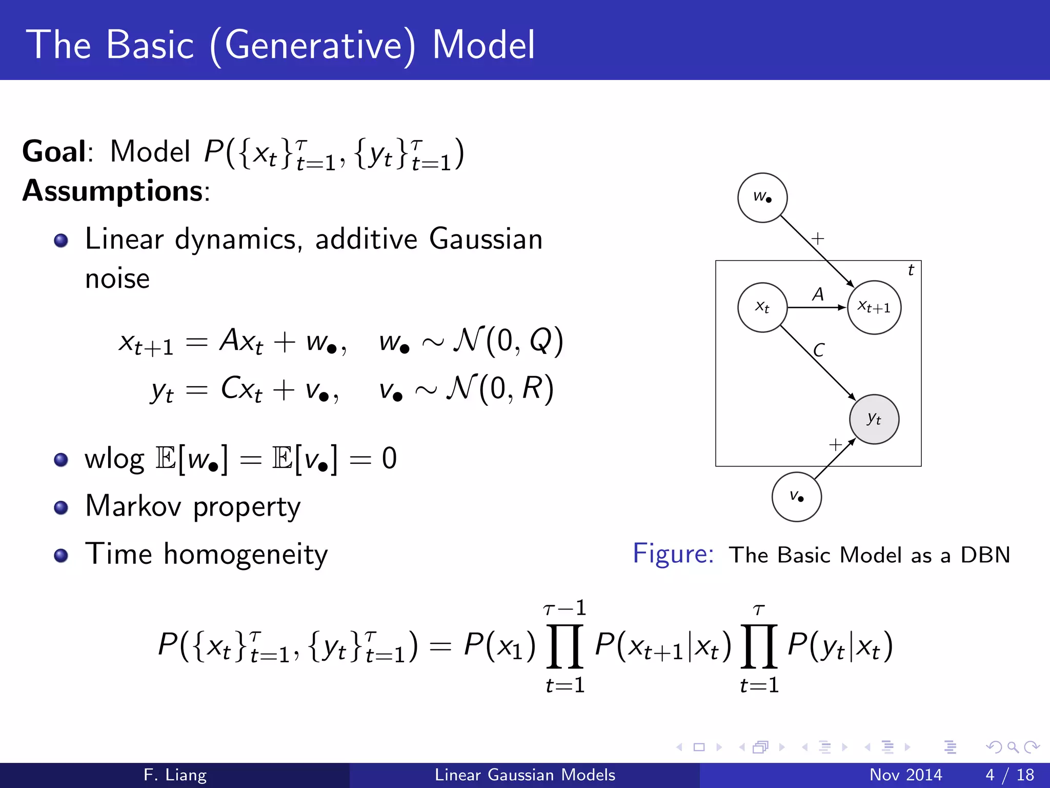
Goal: Model P(fxtgt
=1; fytgt
=1)
Assumptions:
Linear dynamics, additive Gaussian
noise
xt+1 = Axt + w; w N(0;Q)
yt = Cxt + v; v N(0; R)
wlog E[w] = E[v] = 0
Markov property
Time homogeneity
w
+
xt xt+1
yt
v
A
C
+
t
Figure: The Basic Model as a DBN
P(fxtgt
=1; fytgt
=1) = P(x1)
Y1
t=1
P(xt+1jxt )
Y
t=1
P(yt jxt )
F. Liang Linear Gaussian Models Nov 2014 4 / 18

6. Why Gaussians?
Gaussian family closed under ane transforms
x N(x ;x ); y N(y ;y ); a; b; c 2 R
=) ax + by + c N(ax + by + c; a2x + b2y )
Gaussian is conjugate prior for Gaussian likelihood
P(x) Normal; P(yjx) Normal =) P(xjy) Normal
F. Liang Linear Gaussian Models Nov 2014 5 / 18

7. The Inference Problem
Given the system model and initial distribution (fA; C;Q; R; 1;Q1g):
Filtering: P(xt jfyigti
=1)
Smoothing: P(xt jfyigi
=1) where t
If we had the partition function:
P(fyigi=1) =
Z
8fxi gi
=1
P(fxig; fyig)dfxig
Then
P(xt jfyigi
=1) =
P(fxig; fyig)
P(fyig)
F. Liang Linear Gaussian Models Nov 2014 6 / 18

8. The Learning Problem
Let = fA; C;Q; R; 1;Q1g, X = fxigi
=1, Y = fyigi
=1.
Given (several) observable sequences Y :
arg max L() = arg max log P(Y j)
Solved by expectation maximization.
F. Liang Linear Gaussian Models Nov 2014 7 / 18

9. Expectation Maximixation
For any distribution Q on Sx :
L() F(Q; ) =
Z
X
Q(X) log P(X; Y j)
Z
X
Q(X) logQ(X)dX
= L() + H(Q; P(jY ; )) H(Q)
= L() DKL(QjjP(jY ; ))
Monotonically increasing coordinate ascent on F(Q; ):
E step: Qk+1 arg maxQ F(Q; k ) = P(XjY ; k )
M step: k+1 arg max F(Qk+1; )
F. Liang Linear Gaussian Models Nov 2014 8 / 18

10. Continuous-State Static Modeling
Assumptions:
x is continuously supported
A = 0
x = w N(0;Q) =) y = Cx + v N(0;CQCT + R)
wlog Q = I
Ecient Inference Using Sucient Statistics: Gaussian is conjugate
prior for Gaussian likelihood, so
P(xjy) = N(

11. y; I

12. C);

13. = CT (CCT + R)1
Learning: R must be constrained to avoid degenerate solution. . .
F. Liang Linear Gaussian Models Nov 2014 9 / 18

14. Continuous-State Static Modeling: Factor Analysis
y = Cx + v N(0; CCT + R)
Additional Assumption:
R diagonal =) observation noise v independent along basis for y
Interpretation:
R : variance along basis
C : correlation structure of latent factors
Properties:
Scale invariant
Not rotation invariant
F. Liang Linear Gaussian Models Nov 2014 10 / 18

15. Continuous-State Static Modeling: SPCA and PCA
y = Cx + v N(0; CCT + R)
Additional Assumptions:
R = I ; 2 R
For PCA: R = lim!0 I
Interpretation:
: global noise level
Columns of C : principal components
(optimizes three equivalent objectives)
Properties
Rotation invariant
Not scale invariant
F. Liang Linear Gaussian Models Nov 2014 11 / 18

16. Continuous-State Dynamic Modeling: Kalman Filters
Relax A = 0 assumptio.
Optimal Bayes

17. lter assuming linearity and normality (conjugate prior)
F. Liang Linear Gaussian Models Nov 2014 12 / 18

18. Discrete-State Modeling: Winner-Takes-All (WTA)
Non-linearity
Assume: x discretely supported,
R
7!
P
Winner-Takes-All Non-Linearity: WTA[x] = ei where i = arg maxj xj
xt+1 = WTA[Axt + w] w N(;Q)
yt = Cxt + v v N(0; R)
x WTA[N(; )] de

19. nes a probability vector where i = P(x = ei ) =
probability mass assigned by N(; ) to fz 2 Sx : 8j6= i : (z)i (z)jg
F. Liang Linear Gaussian Models Nov 2014 13 / 18

20. Static Discrete-State Modeling: Mixture of Gaussians and
Vector Quantization
x = WTA[w] w N(;Q)
y = Cx + v v N(0; R)
Additional Assumption: A = 0
Mixture of Gaussians:
P(y) =
X
i
P(x = ej ; y) =
X
i
N(Ci ; R)i
All Gaussians have same covariance R
Inference:
P(x = ej jy) =
P(x = ej ; y)
P(y)
=
PN(Cj ; R)j
i N(Ci ; R)i
Vector Quantization: R = lim!0 R0
F. Liang Linear Gaussian Models Nov 2014 14 / 18

21. Dynamic Discrete-State Modeling: Hidden Markov Models
xt+1 = WTA[Axt + w] w N(0;Q)
yt = Cxt + v v N(0; R)
Theorem
Any Markov chain transition dynamics T can be equivalently modeled
using A and Q in the above model and vice versa.
All states have same emission covariance R
Learning: EM Algorithm (Baum-Welch)
Inference: Viterbi Algorithm for MAP estimate
In discrete case, MAP estimate6= least-squares estimate
Approaches Kalman

22. ltering as discretization gets

23. ner
F. Liang Linear Gaussian Models Nov 2014 15 / 18

24. Conclusions
Linearity and normality =) computationally tractable
Universal basic model generalizes idiosyncratic special cases and
highlights relationships (e.g. static vs dynamic, zero noise limit,
hyperparameter selection)
Uni

25. ed set of equations and algorithms for inference and learning
F. Liang Linear Gaussian Models Nov 2014 16 / 18

26. Critique / Future Work
Critique:
Uni

27. ed algorithms not the most ecient
Can only model y with support Rp, x with support Rk or f1; : : : ; ng
Future Work:
Increase hierarchy beyond two levels (e.g. Speech ! n-gram !
PCFG)
Relax time homogeneity assumption (e.g. Extended Kalman Filter)
Extend to other distributions
Try other (likelihood,conjugate prior) pairs
Approximate inference (MH-MCMC)
F. Liang Linear Gaussian Models Nov 2014 17 / 18

28. References
S. Roweis, Z. Ghahramani.
A Unifying Review of Linear Gaussian Models.
Computation and Neural Systems, 11(2):305{345, 1999.
Image Attributions:
http://www.robots.ox.ac.uk/ parg/projects/ica/riz/Thesis/Figs/var/MoG.jpeg
https://github.com/echen/restricted-boltzmann-machines
http://upload.wikimedia.org/wikipedia/commons/1/15/GaussianScatterPCA.png
http://www.ee.columbia.edu/ln/LabROSA/doc/HTKBook21/img15.gif
http://commons.wikimedia.org/wiki/File:Basic concept of Kalman

29. ltering.svg
http://learning.cis.upenn.edu/cis520 fall2009/uploads/Lectures/pca-example-1D-of-2D.png
F. Liang Linear Gaussian Models Nov 2014 18 / 18