This document discusses various machine learning methods that have been applied to computer architecture problems. It begins by introducing k-means clustering and how it is used in SimPoint to reduce architecture simulation time. It then discusses how machine learning can be used for design space exploration in multi-core processors and for coordinated resource management on multiprocessors. Finally, it provides an example of using artificial neural networks to build performance models to inform resource allocation decisions.

1. A Survey of Machine Learning Methods
Applied to Computer Architecture
Balaji Lakshminarayanan
lakshmba@eecs.oregonstate.edu
Paul Lewis
lewisp@eecs.oregonstate.edu
Introduction
2
Architecture Simulation
2
K-means Clustering
3
Design Space Exploration
6
Coordinated Resource Management on Multiprocessors
7
Artificial Neural Networks
9
Hardware Predictors
11
Decision Tree Learning
12
Learning Heuristics for Instruction Scheduling
14
Other Machine Learning Methods
18
Online Hardware Reconfiguration
18
GPU
18
Data Layout
18
Emulate Highly Parallel Systems
19
References
19

2. Introduction
Machine learning is the subfield of artificial intelligence that is concerned with the design
and development of data based algorithms that improve in performance over time. A
major focus of machine learning research is to automatically induce models, such as
rules and patterns, from data. In computer architecture, many resources interact with
each other and building an exact model can be very difficult for even a simple
processor. Hence, machine learning methods can be applied to automatically induce
models. In this paper we look for ways in which machine learning has been applied to
various aspects of computer architecture and analyze the current and future influence of
machine learning in this field.
Taxonomy of ML algorithms
Machine learning algorithms are organized into a taxonomy based on the desired
outcome of the algorithm. The following is a list of common algorithm types used in this
paper.
• Supervised learning - in which the algorithm generates a function that maps inputs to
desired outputs. One standard formulation of the supervised learning task is the
classification problem: the learner is required to learn (to approximate) the behavior of
a function which maps a vector into one of several classes by looking at several input-
output examples of the function. It may be difficult to get properly labeled data in many
scenarios. Also, if the training data is corrupted, the algorithm may not learn the
correct function. The ʻlearning algorithmʼ needs to be robust to noise in training data,
e.g. artificial neural networks and decision trees.
• Unsupervised learning - in which the algorithm models a set of inputs where labeled
examples are not available. In this case, the inputs are grouped into clusters based on
some relative similarity measure. The performance may not be as good as the
Supervised case, but itʼs much easier to get unlabeled examples than labeled data,
e.g. k-means clustering.
• Semi-supervised learning - which combines both labeled and unlabeled examples to
generate an appropriate function or classifier.
• Reinforcement learning - in which the algorithm learns a policy of how to act given an
observation of the world. Every action has some impact in the environment, and the
environment provides feedback that guides the learning algorithm.
Architecture Simulation
Architecture simulators typically model each cycle of a specific program on a given
hardware design using software. This modeling is used to gain information about a
hardware design such as the average CPI and cache miss rates; it can be a time
consuming process taking days or weeks just to run a single simulation. It is common
for a suite of programs to be tested against a set of architectures. This is a problem

3. since it can take weeks for just a single test and several of these tests need to be
performed taking months.
SPEC (Standard Performance Evaluation Corporation) is one of many industry standard
tests that allow the performance of various architectures to be compared. Spec
consists of a suite of 26 programs, 12 integer and 14 floating point.
Simple Scalar is a standard industry simulator that is used to compare results to
SimPoint a machine learning approach simulation. It simulates each cycle of the
running program and records CPI, cache miss rates, branch miss prediction and power
consumption.
SimPoint is a machine learning approach to architecture simulation that uses k-means
clustering. It exploits the structured way in which individual programs behavior changes
over time. In this way it selects a set of samples called simulation points that represent
every type of behavior in a program. These samples are then weighted by the amount
of behavior these samples represent.
Definitions:
• Interval - a slice of the overall program. The program is divided up into equal sized
intervals; SimPoint usually selects intervals around 100 million instructions.
• Similarity - a metric that represents the similarity in behavior of two intervals of a
programs execution.
• Phase (Cluster) - A set of intervals in a program that have similar behavior regardless
of temporal location.
K-means Clustering
K-means clustering takes a set of data points that have n features and uses some kind
of formula to define the similarity. This can be complex and needs to be defined before
hand. Then it clusters the data into K groups. K is not necessarily known ahead of time
and some tests need to be run to figure out a good value of K since too low a value of K
will cause under-fitting of data and too high a value will cause over-fitting.

4. This is an example of K-means clustering applied to two dimensional data points where K = 4.
Assume each point in the example above represented the (x,y) location of a house that
a mailman needs to travel to to make a delivery. The distance could be represented as
the straight line distance between those locations or some kind of street block distance.
Then in order to assign each mailman to a group of houses the K-means clustering
would take in K as the number of available mailmen and build clusters of those houses
that are closest together or have the highest similarity.
SimPoint Design
SimPoint uses an architecture independent metric to classify phase. It clusters data
together based on the program behavior at each interval. This means that while using a
benchmark such as SPEC the clustering of data can be done once over all 26 programs
and then when an architecture is tested on the given programs the same clustering of
phases is used. Since the clustering is independent of architecture features such as
cache miss rate there is no need to recompute the clustering for each architecture
saving a great deal of time.

5. This figures compares the CPI, BBV and phase over the coarse of a specific program.
Using the graph above one can see how k-means clustering is done in SimPoint. First
the trillion instructions of the program are divided into equal intervals of about 100
million instructions each. A sample is take from each interval and its average CPI is
measured as shown in the graph at the top. The second graph shows the similarity
between basic block vectors (BBV). In SimPoint the BBV represents the behavior of an
interval. The last graph shows how the intervals are clustered into four different clusters
in this case (k=4). Where the intervals are similar in graph 2 they are clustered together
in graph 3.
Results
SimPoint has an average error rate over SPEC of about 6%. The figure below shows
some of the programs and their error rates.
The bars are the prediction error of average CPI with respect to a complete cycle by cycle
simulation. The blue bars only sample the first few hundred million cycles while the black bars

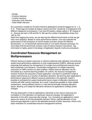
6. skip the first billion instructions and sample the rest of the program. The white bars are the error
associated with SimPoint.
The overall error rate is important but what is far more important given a significantly
high error rate is that the bias of the error from one architecture to another is the same.
The reason for this is that if the bias of error is the same between architectures then
regardless of the magnitude of the error they can be compared fairly without having to
run a reference trial.
Machine learning has the potential to take simulation running time from months to days
or even hours. This is a significant time savings for development and has potential to
become the choice used in industry. SimPoint is being used in industry by companies
such as Intel [1].
Design Space Exploration
As multi-core processor architectures with tens or even hundreds of cores, not all of
them necessarily identical, become common, the current processor design methodology
that relies on large-scale simulations is not going to scale well because of the number of
possibilities to be considered. In the previous section, we saw how time consuming it
can be to evaluate the performance of a single processor. Performance evaluation can
be even trickier with multicore processors. Consider the design of a k-core chip
multiprocessor where each core can be chosen from a library of n cores. There are nk
designs possible. If n = 100 and k = 4, there are totally 10 million possibilities. We see
that the design space explodes even for very small n and k. It is obvious that we need
to find a smart way to choose the ʻbestʼ from these nk designs. We need intelligent/
efficient techniques to navigate through the processor design space. There are two
approaches to tackle this problem
1. Reduce the simulation time for a single design configuration. Techniques like
SimPoint can be used to approximately predict the performance.
2. Reduce the number of configurations tested. In this case, only a small number of
configurations are tested, i.e. the search space is pruned. At each point, the
algorithm moves to a new configuration in a direction that increases the performance
by the maximum amount. This can be thought of as a Steepest Ascent Hill Climbing
algorithm. The algorithm may get stuck at local maxima. To overcome this, one may
employ Hybrid Start Hill Climbing, wherein the Steepest Ascent Hill Climbing is
initiated at several initial points. Each initial point will converge to a local maxima and
the global maximum is the maximum amongst these local maxima. Other search
techniques such as Genetic Algorithm, Ant Colony Optimization may also be applied.
In reality, all the nk configurations may not be very different from each other. So, we can
group processors based on some relative similarities. One simple method is k-tuple
Tagging. Each processor is characterized by the following parameters ( k=5 here)

7. • Simple
• D-cache intensive
• I-Cache intensive
• Execution units intensive
• Fetch Width intensive
So a processor suitable for D-cache intensive applications would be tagged as ( 0, 1, 0,
0, 0). These tags are treated as feature vectors and then ʻclusteringʼ is employed to find
different categories of processors. If we have M clusters, design space is Mk instead of
nk . Assume we had n=100 and M=10. We see the number of possibilities drops from
1004 to 104!
Apart from tagging the cores, we can also tag the different benchmarks so that we get
even more speedup. Based on some performance criterion, one may evaluate the
performance of the processors on the M clusters and then cluster the different
benchmarks. I.e. if a benchmark performs best on a D-cache intensive processor, itʼs
more likely that the benchmark contains many D-cache intensive instructions. Tag
information is highly useful in the design of Application Specific multi-core processors
Coordinated Resource Management on
Multiprocessors
Efficient sharing of system resources is critical to obtaining high utilization and enforcing
system-level performance objectives on chip multiprocessors (CMPs). Although several
proposals that address the management of a single micro-architectural resource have
been published in the literature, coordinated management of multiple interacting
resources on CMPs remains an open problem. Global resource allocation can be
formulated as a machine learning problem. At runtime, the resource management
scheme monitors the execution of each application, and learns a predictive model of
system performance as a function of allocation decisions. By learning each applicationʼs
performance response to different resource distributions, this approach makes it
possible to anticipate the system-level performance impact of allocation decisions at
runtime with little runtime overhead. As a result, it becomes possible to make reliable
comparisons among different points in a vast and dynamically changing allocation
space, allowing us to adapt the allocation decisions as applications undergo phase
changes.
The key observation is that an applicationʼs demands on the various resources are
correlated i.e if the allocation of a particular resource changes, the applicationʼs
demands on the other resources also change. E.g. increasing an applicationʼs cache
space can reduce its off-chip bandwidth demand. Hence, optimal allocation of one
resource type depends in part on the allocated amounts of other resources, which is the
basic motivation for coordinated resource management scheme.

8. The above figure shows an overview of the resource allocation framework, which
comprises per-application hardware performance models, as well as a global resource
manager. Shared system resources are periodically redistributed between applications
at fixed decision-making intervals, allowing the global manager to respond to dynamic
changes in workload behavior. Longer intervals amortize higher system reconfiguration
overheads and enable more sophisticated (but also more costly) allocation algorithms,
whereas shorter intervals permit faster reaction time to dynamic changes. At the end of
every interval, the global manager searches the space of possible resource allocations
by repeatedly querying the application performance models. To do this, the manager
presents each model a set of state attributes summarizing recent program behavior,
plus another set of attributes indicating the allocated amount of each resource type. In
turn, each performance model responds with a performance prediction for the next
interval. The global manager then aggregates these predictions into a system-level
performance prediction (e.g., by calculating the weighted speedup across all
applications). This process is repeated for a fixed number of query-response iterations
on different candidate resource distributions, after which the global manager installs the
configuration estimated to yield the highest aggregate performance. Successfully
managing multiple interacting system resources in a CMP environment presents several
challenges. The number of ways a system can be partitioned among different
applications grows exponentially with the number of resources under control, leading to
over one billion possible system configurations in a quad-core setup with three
independent resources. Moreover, as a result of context switches and application phase
behavior, workloads can exert drastically different demands on each resource at
different points in time. Hence, optimizing system performance requires us to quickly
determine high-performance points in a vast allocation space, as well as anticipate and
respond to dynamically changing workload demands.

9. Artificial Neural Networks
Artificial Neural Networks (ANNs) are machine learning models that automatically learn
to approximate a target function (application performance in our case) based on a set of
inputs.
The above figure shows an example ANN consisting of 12 input units, four hidden units,
and an output unit. In a fully connected feed-forward ANN, an input unit passes the data
presented to it to all hidden units via a set of weighted edges. Hidden units operate on
this data to generate the inputs to the output unit, which in turn calculates ANN
predictions. Hidden and output units form their results by first taking a weighted sum of
their inputs based on edge weights, and by passing this sum through a non-linear
activation function.
Increasing the number of hidden units in an ANN leads to better representational power
and the ability to model more complex functions, but increases the amount of training

10. data and time required to arrive at accurate models. ANNs represent one of the most
powerful machine learning models for non-linear regression; their representational
power is high enough to model multi-dimensional functions involving complex
relationships among variables.
Each network takes as input the amount of L2 cache space, off-chip bandwidth, and
power budget allocated to its application. In addition, networks are given nine attributes
describing recent program behavior and current L2-cache state.
These nine attributes are:
Number of (1) read hits, (2) read misses, (3) write hits, and (4) write misses in the L1
d-Cache over the last 20K instructions; Number of (5) read hits, (6) read misses, (7)
write hits, and (8) write misses in the L1 d-Cache over the last 1.5M instructions; and (9)
the fraction of cache ways allocated the modeled application that are dirty.
The first four attributes are intended to capture the programʼs phase behavior in the
recent past, whereas the next four attributes summarize program behavior over a longer
time frame. Summarizing program execution at multiple granularities allows us to make
accurate predictions for applications whose behaviors change at different speeds. Using
L1 d-Cache metrics as inputs allows us to track the applicationʼs demands on the
memory system without relying on metrics that are affected by resource allocation
decisions. The ninth attribute is intended to capture the amount of write-back traffic that
the application may generate; an application typically generates more write-back traffic
if it is allocated a larger number of dirty cache blocks.
Results
The above figure shows an example of performance loss due to uncoordinated resource
management in a CMP where three resources (cache, BW, power and combinations of
them) are shared. A four-application, desktop style multiprogrammed workload is
executed on a quad-core CMP with an associated DDR2-800 memory subsystem.
Performance is measured in terms of weighted speedup (ideal weighted speedup here
is 4, which corresponds to all four applications executing as if they had all the resources
to themselves). Configurations that dynamically allocate one or more of the resources in
an uncoordinated fashion (Cache, BW,Power, and combinations of them) are compared

11. to a static, fair-share allocation of the resources (Fair-Share), as well as an unmanaged
sharing scenario (Unmanaged), where all resources are fully accessible by all
applications at all times. We see that co-ordinated management of all 3 resources
Cache, BW, Power is still worse than the static fair-share allocation. However, we can
build models for resource allocation profiles for different applications. If we had these
models, we can certainly expect the dynamic resource allocation to perform better.
Hardware Predictors
Hardware predictors are used to make quick predictions of some unknown value that
otherwise would take much longer to compute and waste clock cycles. If a predictor
has a high enough detection rate the expected saved time by using it can be significant.
There are many uses for predictors in computer architecture including branch
predictors, value predictors, memory address predictors and dependency predictors.
These predictors all work in hardware at real time to improve performance.
Despite the fact that current table based branch predictors can achieve upward of 98%
prediction accuracy research is still being done to analyze and improve upon current
methods. Recently some machine learning methods have been applied, specifically
decision tree learning. We found a paper that uses decision tree based machine
learning to predict values based on smaller subsets of the overall feature space. The
methods used in this paper could be applied to other types of hardware predictors and
at the same time improved upon by using some sort of hybrid approach with classic
table based predictors.
Current table based predictors do not scale well so the number of features is limited.
This means that although the average prediction rate is higher there are some
behaviors that the low featured table based predictors cannot handle. A table based
predictor typically has a small set of features because for each feature, n, that it has
there are 2n feature vectors, each of which it must represent in memory. This means
that the table size increases exponentially with the increase in feature size.
Previous papers have shown that prediction using a subset of features is nearly as good
if the features are carefully chosen. A study was done where predictions were
computed by using a large set of features and then a human chose the most promising
subset of features for each branch and predictions were done again. The branch
predictions were nearly as good as when using all the features. This means that by
intelligently choosing a subset of features from a larger set the number of features used
can be greatly increased and the feature set does not need to be known ahead of time.
Definitions
• Target bit - the bit to be predicted
• Target outcome - the value that bit will eventually have
• Feature vector - set of bits used to predict the target bit

12. Decision Tree Learning
Decision trees are used to predict outcomes given a set of features. This set of features
is known as the feature vector. Typically in machine learning the data set consists of
hundreds or thousands of feature vector/target outcome pairs and is processed to
create a decision tree. That tree is then used to predict future outcomes. It is almost
always the case that the number of feature vectors is a small subset of the total number
of potential feature vectors otherwise one could just compare a new feature vector to an
old one and copy the outcome.
This figure illustrates the relationship between binary data and a binary decision tree. The blue
boxes represent positive values and the red boxes are negative values.
In the figure above an example data set of four feature vector/outcome bit pairs is given.
Using this data a tree can be created that splits the data based on any of those
features. It can be seen that F1 splits the data between red and blue without any mixing
(this is ideal). The better a feature is the more information that is gained from dividing
the outcomes based on that features values. It can also be seen that F2 and F3 can be
used together as a larger tree to segregate all the data elements into groups containing
all of the same values.
Noise can be introduced into the data by having two sets of date with the same feature
vectors but different outcomes. This can happen if the features are not representative
of all the possible features.

13. Dynamic Decision Tree (DDT)
The hardware implementation of a decision tree has some issues that need to be dealt
with. In hardware prediction there may not be a nice set of data to start with so the
predictor needs to start predicting right away and update its tree on the fly. One design
for a DDT used for branch prediction stores a counter for each feature and updates that
counter as feature vector/outcome pairs are added. The counter is incremented when
the prediction is the same as the outcome and decremented otherwise.
This figure shows how the outcome bit is logically XOR against each feature vector value and
updates the counter for each of those features.
When the most desirable features are being chosen the absolute value of the feature is
used because a feature that is always wrong ends up being always correct by simply
flipping all the bits and thus can be a very good feature.
This figure shows how the best feature is selected by taking the max absolute value of all the
features.
There are two modes to the dynamic predictor. In prediction mode it takes in a feature
vector and returns a prediction. In update mode it takes in a feature vector and the
target outcome and updates its internal state. It alternates between prediction and
update mode as it first predicts an outcome then then when the real outcome is known it
updates. The figure below shows a high level view of the predictor. The tree is a fixed
size in memory and thus can only deal with a small number of features but since it
selects the features from a large set of features in a table that grows linear in size with
respect to the number of features it doesnʼt need to be very large.

14. View of the high level view of the DDT hardware prediction logic for branch prediction for a
single branch.
Experimentally the decision tree branch prediction method compares well to some
current table based predictors. It does better in some situations and worse in others
and overall does almost as well in the experiments performed. Since machine learning
is used to having lots of data for prediction and in this case it starts off with very limited
data it would take a while for the predictions to become highly accurate the predictions
would eventually do very well.
There is some added hardware complexity to use a decision tree in hardware at each
branch condition rather than a table and getting the learner to act online within certain
time limits can be a challenge. However the size of the hardware can remain relatively
small and only grow linear with respect the the number of features added. I believe this
approach could be useful as a hybrid predictor or in other hardware predictors.
Learning Heuristics for Instruction Scheduling
Execution speed of programs on modern computer architectures is sensitive, by a factor
of two or more, to the order in which instructions are presented to the processor. To
realize potential execution efficiency, it is now customary for an optimizing compiler to
employ a heuristic algorithm for instruction scheduling. These algorithms are
painstakingly hand-crafted, which is expensive and time-consuming. The instruction
scheduling problem can be formulated as a learning task, so that one obtains the
heuristic scheduling algorithm automatically. As discussed in the introduction,
supervised learning requires a sufficient number of correctly labeled examples. If we

15. train on blocks of code (say about 10 instructions each) rather than the entire code
itself, itʼs easier to get large number of optimally scheduled training examples.
A basic block is defined to be a straight-line sequence of code, with a conditional or
unconditional branch instruction at the end. The scheduler should find optimal, or good,
orderings of the instructions prior to the branch. It is safe to assume that the compiler
has produced a semantically correct sequence of instructions for each basic block. We
consider only reordering of each sequence (not more general rewritings), and only
those reorderings that cannot affect the semantics. The semantics of interest are
captured by dependences of pairs of instructions. Specifically, instruction Ij depends on
(must follow) instruction Ii if it follows Ii in the input block and has one or more of the
following dependences on Ii:
(a) Ij uses a register used by Ii and at least one of them writes the register (condition
codes, if any, are treated as a register);
(b) Ij accesses a memory location that may be the same as one accessed by Ii, and at
least one of them writes the location.
From the input total order of instructions, one can thus build a dependence DAG,
usually a partial (not a total) order, that represents all the semantics essential for
scheduling the instructions of a basic block. Figure 1 gives a sample basic block and its
DAG. The task of scheduling is to find a least-cost (cost is typically designed to reflect
the total number of cycles) total order of each blockʼs DAG.
Instruction to be Scheduled

16. Dependency Graph
Two Possible Schedules with Different Costs
One can view this as learning a relation over triples (P;Ii ;Ij), where P is the partial
schedule (the total order of what has been scheduled, and the partial order remaining),
and I is the set of instructions from which the selection is to be made. Those triples that
belong to the relation define pairwise preferences in which the first instruction is
considered preferable to the second. Each triple that does not belong to the relation
represents a pair in which the first instruction is not better than the second. The
representation used here takes the form of a logical relation, in which known examples
and counter-examples of the relation are provided as triples. It is then a matter of
constructing or revising an expression that evaluates to TRUE if (P;Ii ;Ij) is a member of
the relation, and FALSE if it is not. If (P;Ii ;Ij), is considered to be a member of the
relation, then it is safe to infer that (P;Ii ;Ij), is not a member. For any representation of
preference, one needs to represent features of a candidate instruction and of the partial
schedule. The authors used the features described in Table below

17. The choice of features is pretty obvious:
Critical path indicates that another instruction is waiting for the result of this instruction.
Delay refers to the latency associated with a particular instruction.
The authors chose the Digital Alpha 21064 as our architecture for the instruction
scheduling problem. The 21064 implementation of the instruction set is interestingly
complex, having two dissimilar pipelines and the ability to issue two instructions per
cycle (also called dual issue) if a complicated collection of conditions hold. Instructions
take from one to many tens of cycles to execute. SPEC95 is a standard benchmark
commonly used to evaluate CPU execution time and the impact of compiler
optimizations. It consists of 18 programs, 10 written in FORTRAN and tending to use
floating point calculations heavily, and 8 written in C and focusing more on integers,
character strings, and pointer manipulations. These were compiled with the vendorʼs
compiler, set at the highest level of optimization offered, which includes compile- or link
time instruction scheduling. We call these the ʻOrigʼ schedules for the blocks. The
resulting collection has 447,127 basic blocks, composed of 2,205,466 instructions. DEC
refers to the performance of the DEC heuristic scheduler ( hand crafted and performs
the best). Different supervised learning techniques were employed. Even though they
were not as good as handcrafted, they perform reasonably well
• ITI refers to decision tree induction program
• TLU refers to table lookup
• NN refers to artificial neural network

18. The cycle counts are tested under two different conditions. In the first case i.e. ʻRelevant
blocksʼ, only basic blocks are considered for testing. In the second case i.e. ʻAll blocksʼ,
even blocks of length > 10 are included. Even though blocks of length > 10 were not
included during ʻtrainingʼ, we can see that the learning algorithm performs reasonably
well in this case.
Other Machine Learning Methods
Online Hardware Reconfiguration
Online hardware reconfiguration is similar to the coordinated resource management
mentioned earlier in the paper. The difference is that the resources may be managed at
a higher level (operating system) rather then at a low level in hardware. This higher
level management is useful for domains such as web-servers where large powerful
servers can split their resources into several logical machines. In this case there are
some configurations that are more efficient depending on the workload of each logical
machine and reconfiguration dynamically using machine learning can be beneficial
despite reconfiguration costs.
GPU
The graphical processing unit may be exploited for machine learning tasks. Since the
GPU is designed for image processing which takes in a large amount of similar pieces
of data and processes them in parallel it is ideal for machine learning that needs to
process large amounts of data.
There are is also potential to apply machine learning methods to graphics processing.
Machine learning methods can be used to reduce the amount of data that needs to be
processed by the GPU at the cost of some error but this can be justified if the image
quality difference is not noticeable to the human eye.
Data Layout
Memory in most computers is organized hierarchically, from small and very fast cache
memories to large and slower main memories. Data layout is an optimization problem
whose goal is to minimize the execution time of software by transforming the layout of

19. data structures to improve spatial locality. Automatic data layout performed by the
compiler is currently attracting much attention as significant speed-ups have been
reported. The state-of-the-art is that the problem is known to be NP-complete. Hence,
Machine learning methods may be employed to identify good heuristics and improve
overall speedup.
Emulate Highly Parallel Systems
The efficient mapping of program parallelism to multi-core processors is highly
dependent on the underlying architecture. Applications can either be written from
scratch in a parallel manner, or, given the large legacy code base, converted from an
existing sequential form. In [15], the authors assume that program parallelism is
expressed in a suitable language such as OpenMP. Although the available parallelism
is largely program dependent, finding the best mapping is highly platform or hardware
dependent. There are many decisions to be made when mapping a parallel program to
a platform. These include determining how much of the potential parallelism should be
exploited, the number of processors to use, how parallelism should be scheduled etc.
The right mapping choice depends on the relative costs of communication, computation
and other hardware costs and varies from one multicore to the next. This mapping can
be performed manually by the programmer or automatically by the compiler or run-time
system. Given that the number and type of cores is likely to change from generation to
the next, finding the right mapping for an application may have to be repeated many
times throughout an applicationʼs lifetime, thus making Machine learning based
approaches attractive.
References
1. Greg Hamerly. Erez Perelman, Jeremy Lau, Brad Calder and Timothy Sherwood.
Using Machine Learning to Guide Architecture Simulation. Journal of Machine
Learning Research 7, 2006.
2. Sukhun Kang and Rakesh Kumar - Magellan: A Framework for Fast Multi-core
Design Space Exploration and Optimization Using Search and Machine Learning
Proceedings of the conference on Design, automation and test in Europe, 2008
3. R. Bitirgen, E. İpek, and J.F. Martínez - Coordinated management of multiple
resources in chip multiprocessors: A machine learning approach, In Intl. Symp. on
Microarchitecture, Lake Como, Italy, Nov. 2008.
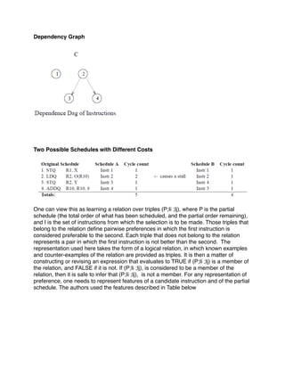
4. Moss, Utgoff et al - Learning to Schedule Straight-Line Code NIPS 1997.
5. Malik, Russell et al - Learning Heuristics for Basic Block Instruction Scheduling,
Journal of Heuristics archive. Volume 14 , Issue 6 (December 2008).

20. 6. Alan Fern, Robert Givan, Babak Falsafi, and T. N. Vijaykumar. Dynamic Feature
Selection for Hardware Prediction. Journal of Systems Architecture 52, 4, 213-234,
2006.
7. Alan Fern and Robert Givan. Online Ensemble Learning: An Empirical Study.
Machine Learning Journal (MLJ), 53(1/2), pp. 71-109, 2003.
8. Jonathan Wildstrom, Peter Stone, Emmett Witchel, Raymond J. Mooney and Mike
Dahlin. Towards Self-Configuring Hardware for Distributed Computer Systems.
ICAC, 2005.
9. Jonathan Wildstrom, Peter Stone, Emmett Witchel and Mike Dahlin. Machine
Learning for On-Line Hardware Reconfiguration. IJCAI, 2007.
10. Jonathan Wildstrom, Peter Stone, Emmett Witchel and Mike Dahlin. Adapting to
Workload Changes Through On-The-Fly Reconfiguration. Technical Report, 2006.
11. Tejas Karkhanis. Automated Design of Application-Specific Superscalar Processors.
University of Wisconsin Madison, 2006.
12. Sukhun Kang and Rakesh Kumar. Magellan: A Framework for Fast Multi-core
Design Space Exploration and Optimization Using Search and Machine Learning.
Design, Automation and Test in Europe, 2008.
13. Matthew Curtis-Maury et al. Identifying Energy-Efficient Concurrency Levels Using
Machine Learning. Green Computer, 2007.
14. Mike O'Boyle: Machine Learning for automating compiler/architecture co-design
Presentation slides, Institute of Computer Systems Architecture. School of
Informatics, University of Edinburgh.
15. Zheng Wang et al: Mapping parallelism to multi-cores: a machine learning based
approach. Proceedings of the 14th ACM SIGPLAN symposium on Principles and
practice of parallel programming, 2009.
16. Peter Van Beek. http://ai.uwaterloo.ca/~vanbeek/research.html.
17. Wikipedia. http://en.wikipedia.org/wiki/Machine_learning.