Download as PDF, PPTX
![1/16
GCT Semiconductor, Inc.
RFIT 2022
Table of Contents
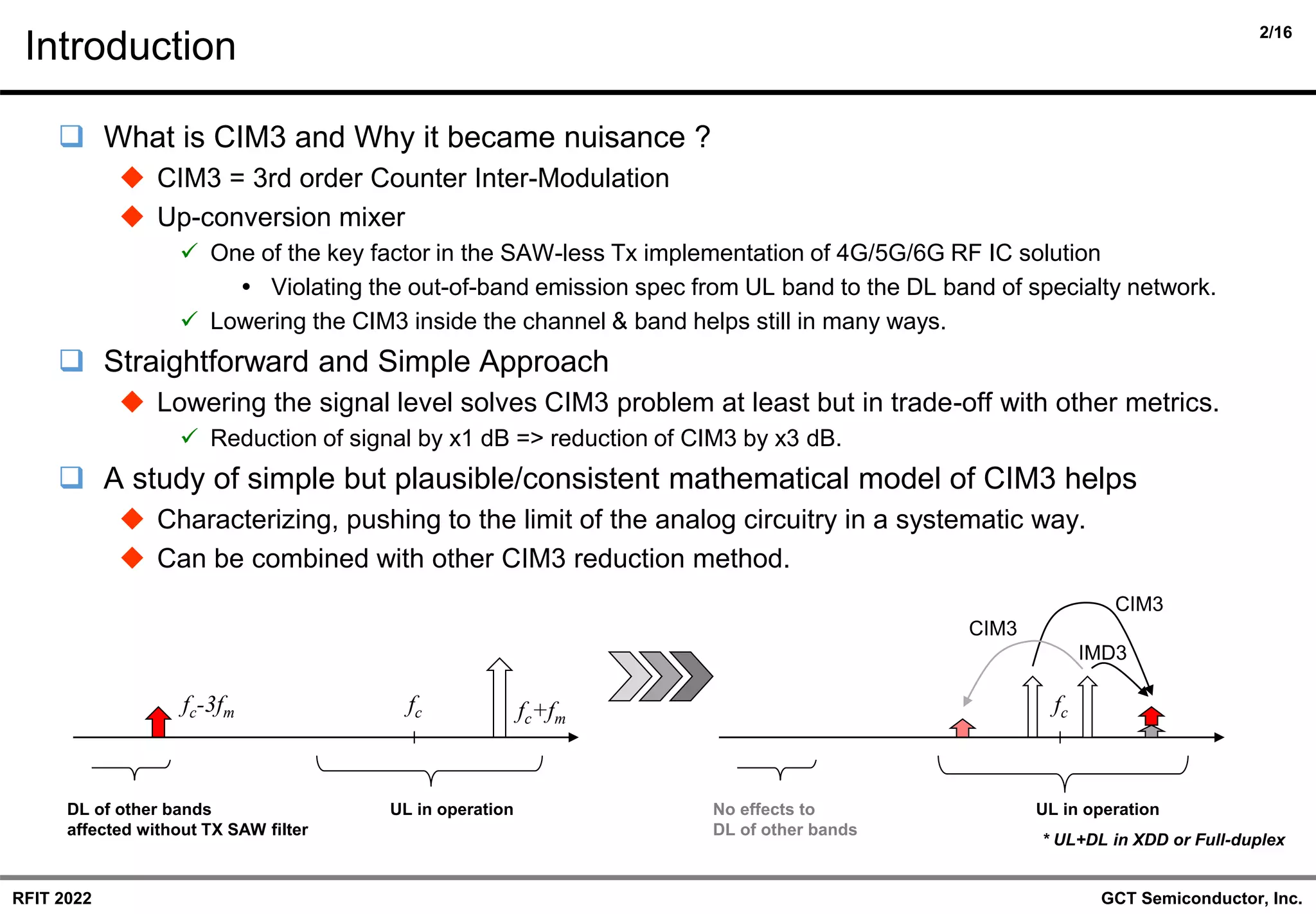
❑ Introduction
◆ Meaning of the study on the CIM3-only DPD model.
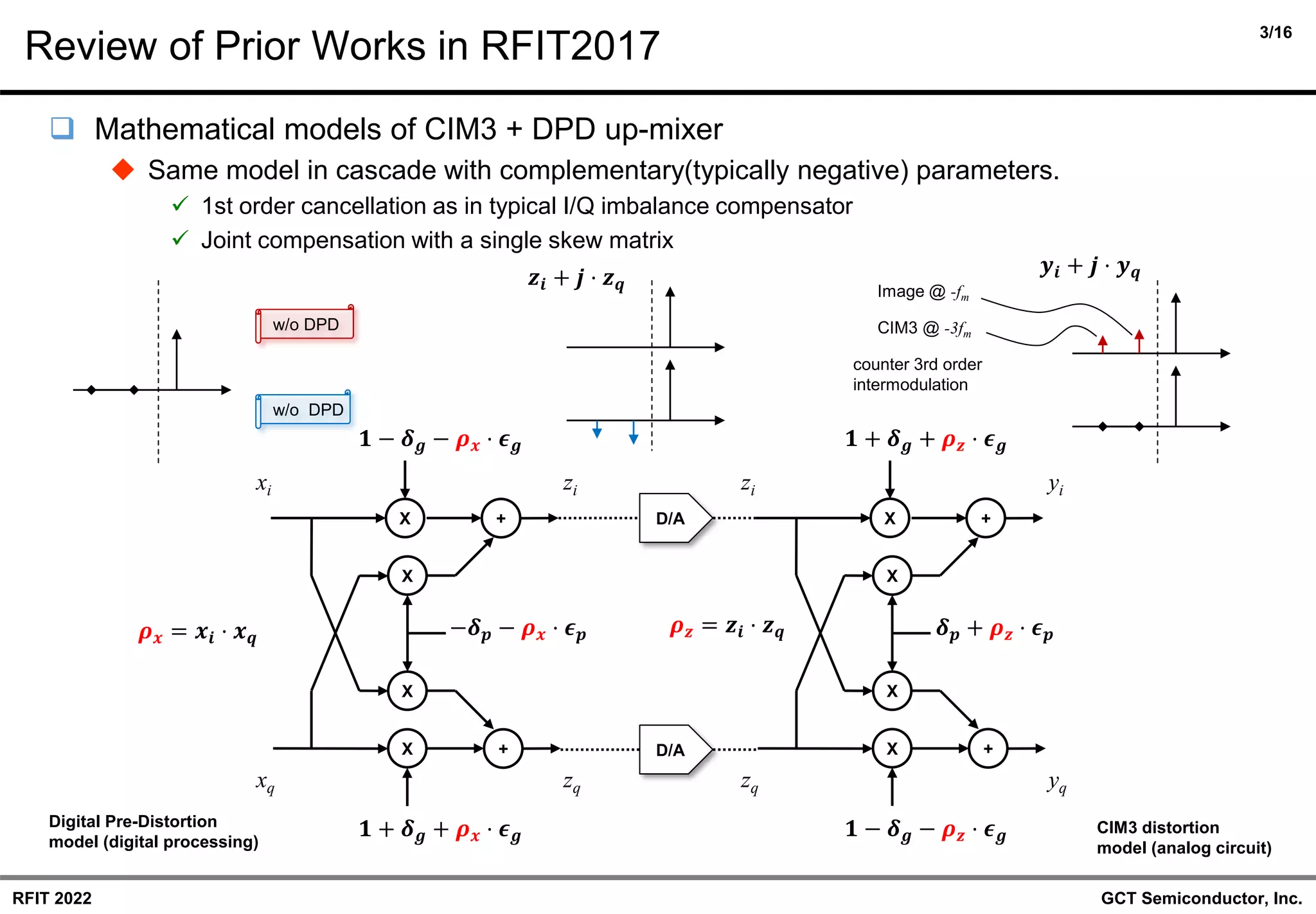
◆ Review of the previous work of joint I/Q-imbalance and CIM3 model.
❑ Duality between the components of I/Q gain/phase mismatch
◆ Review of the duality in I/Q imbalance model.
◆ Extension and application to CIM3 model with conjugate signal representation
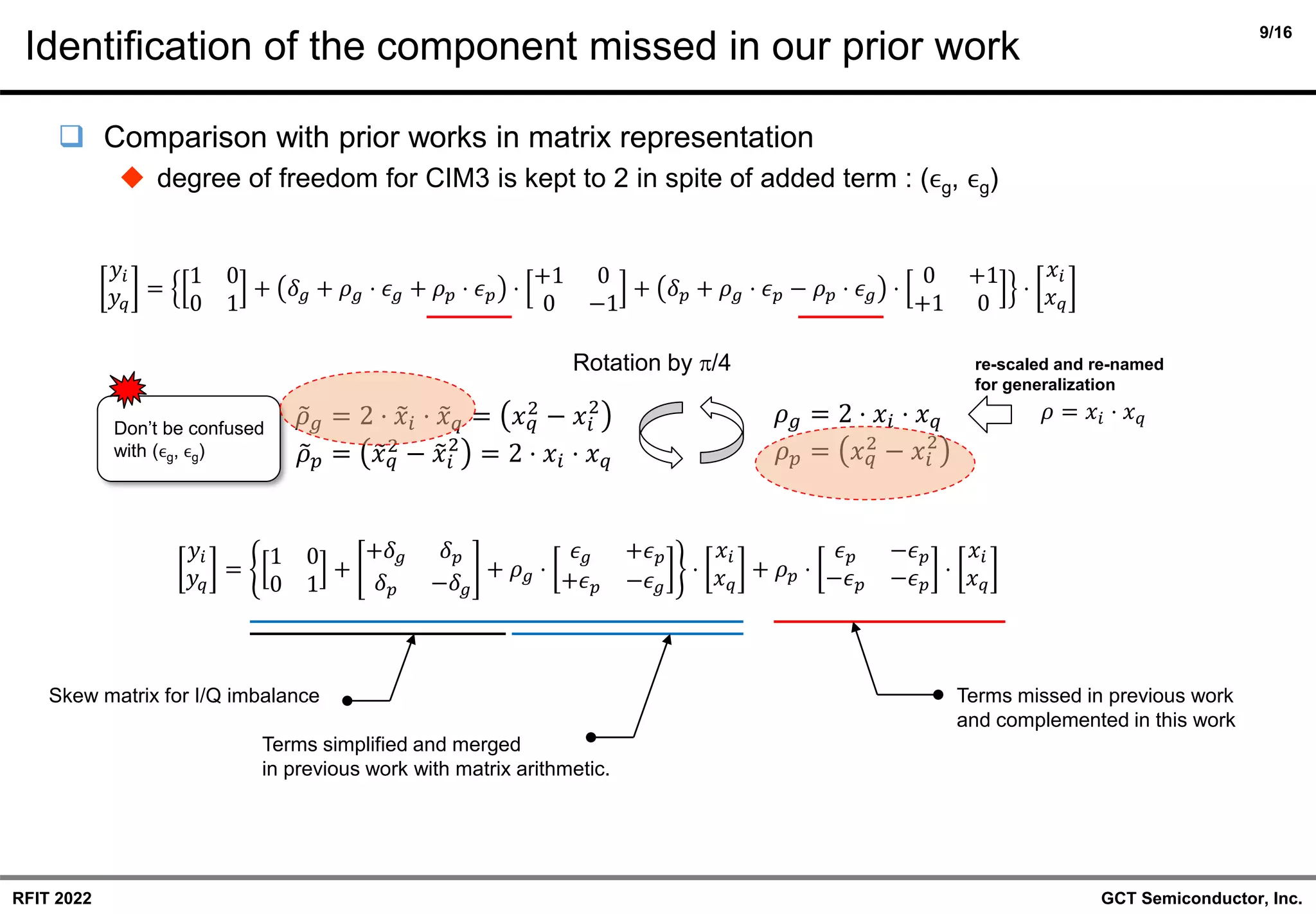
❑ Correction/Enhancement to the CIM3 models introduced in 5 years ago
◆ Identification of missing terms in prior works.
◆ Evaluation of the improvement after the correction.
❑ LMS adaptation revisited and its simplification
◆ Frequency domain => Time domain : Parseval’s theorem
◆ Link to other works already established for I/Q imbalance : circularity
❑ Conclusion
◆ Refined version of joint CIM3 + I/Q imbalance model
[ pp. 2 ~ 5 ]
[ pp. 6 ~ 8 ]
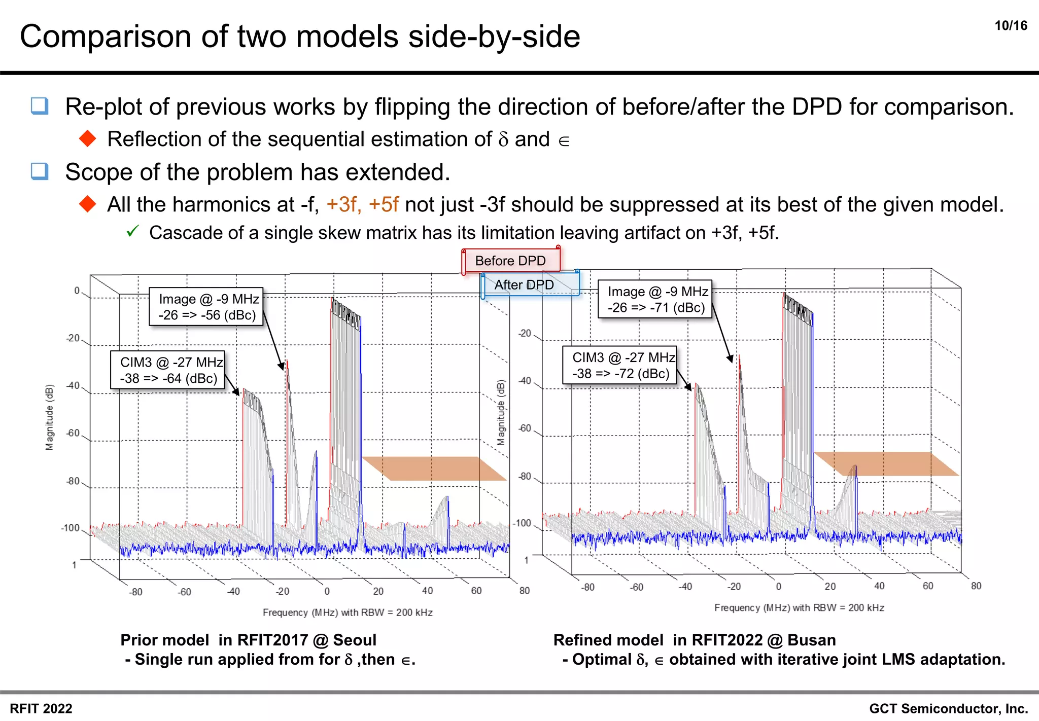
[ pp. 9 ~ 10 ]
[ pp. 11 ~ 15 ]
[ p. 16 ]](https://image.slidesharecdn.com/rfit2022-ealwanleet3b4-220828055639-285914d3/75/A-Refined-Skew-Matrix-Model-of-the-CIM3-in-the-Up-Mixer-Extending-the-Duality-of-I-Q-Imbalance-RFIT-2022-2-2048.jpg)
![6/16
GCT Semiconductor, Inc.
RFIT 2022
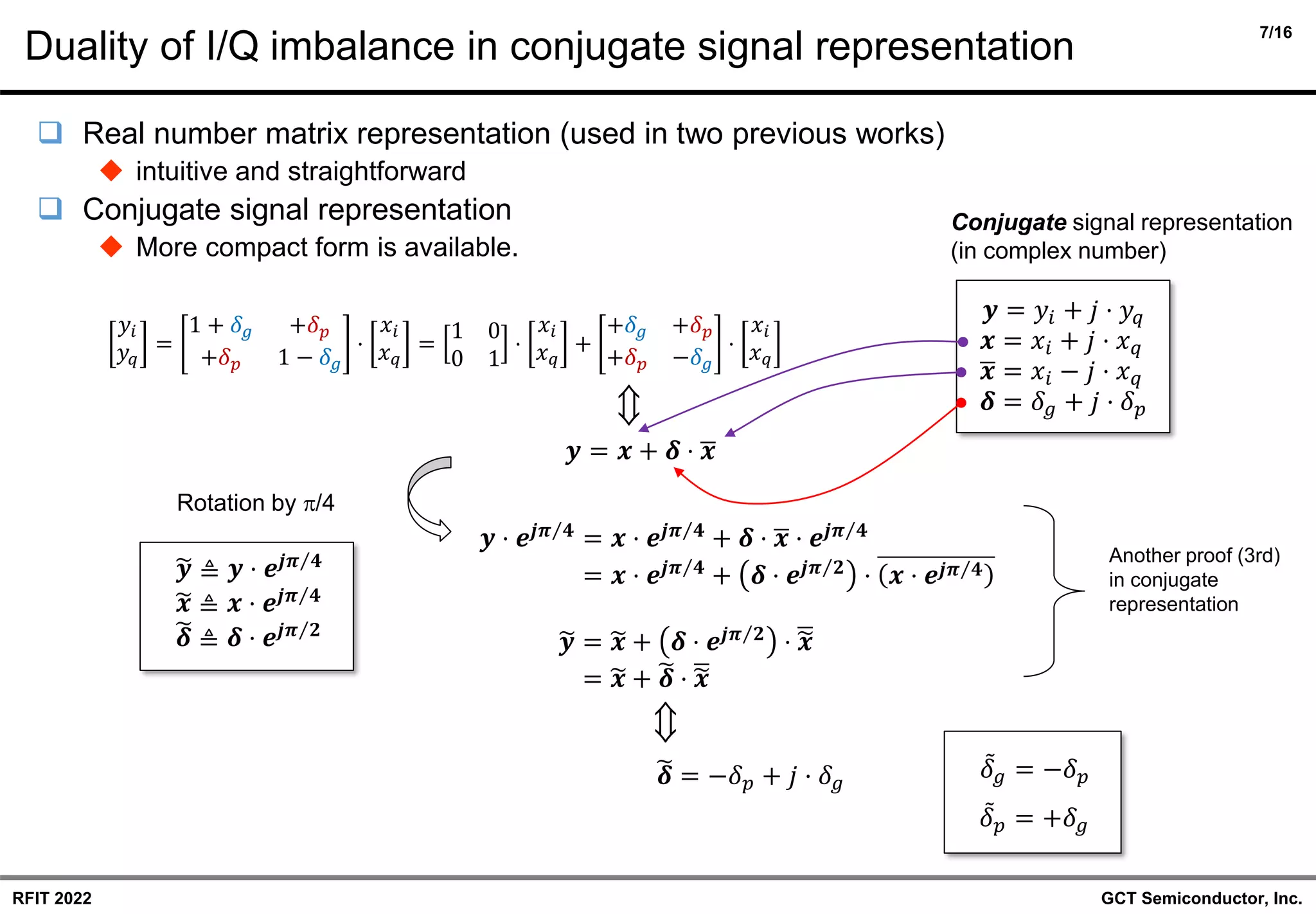
Duality of I/Q imbalance model in the (down)-mixer
❑ gain mismatch(ϵg) and phase mismatch(ϵp) are exchangeable under signal rotation.
◆ explaining the consistency of image signal and IRR in spectrum against co-ordinate rotation.
Another proof by (2nd)
geometric interpretation
Down-mixer [2018]
1. L1-norm based
LMS calibration
2. Completeness of
symmetric skew matrix
Applied to up-mixer
in this paper.
(ϵg/2, ϵg/2) => (g,g)
Proof by (1st)
simple arithmetic](https://image.slidesharecdn.com/rfit2022-ealwanleet3b4-220828055639-285914d3/75/A-Refined-Skew-Matrix-Model-of-the-CIM3-in-the-Up-Mixer-Extending-the-Duality-of-I-Q-Imbalance-RFIT-2022-7-2048.jpg)
![12/16
GCT Semiconductor, Inc.
RFIT 2022
Derivation of LMS Adaptation Formulae (cont’d)
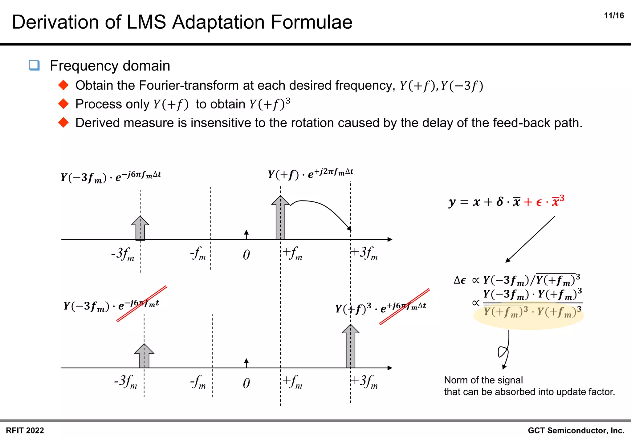
❑ Frequency domain
◆ How to align the desired and distorted component with the same offset from carrier(DC) ?
◆ Squaring in time-domain => Convolution in freq-domain.
✓ Previous method did not pre-processed time-domain signal before DFT.
✓ This measure is also insensitive to the rotation caused by the delay of the feed-back path.
❑ Frequency domain => Time domain : next page
𝒚[𝒏]𝟐
+fm +2fm
-3fm -fm 0
𝒀(+𝒇𝒎)𝟐
∙ 𝒆+𝒋𝟒𝝅𝒇𝒎𝒕
-2fm
𝒀(−𝟑𝒇𝒎)∙𝒀(+𝒇𝒎)∙𝒆−𝒋𝟒𝝅𝒇𝒎𝒕
-6fm
+fm +2fm
-3fm -fm 0
𝒀(−𝟑𝒇𝒎) ∙ 𝒆−𝒋𝟔𝝅𝒇𝒎𝒕
𝒀(+𝒇𝒎)∙𝒆+𝒋𝟐𝝅𝒇𝒎𝒕
-2fm
𝒚[𝒏]
∆𝝐 ∝ 𝒀 −𝟑𝒇𝒎 ⋅ 𝒀 𝒇𝒎
𝟑
∝ 𝒀(−𝟑𝒇𝒎) ⋅ 𝒀(𝒇𝒎) ⋅ 𝒀(𝒇𝒎)𝟐
+𝟐 ⋅ 𝒇𝒎
−𝟐 ⋅ 𝒇𝒎
+𝟐 ⋅ 𝒇𝒎
−𝟐 ⋅ 𝒇𝒎](https://image.slidesharecdn.com/rfit2022-ealwanleet3b4-220828055639-285914d3/75/A-Refined-Skew-Matrix-Model-of-the-CIM3-in-the-Up-Mixer-Extending-the-Duality-of-I-Q-Imbalance-RFIT-2022-13-2048.jpg)
![13/16
GCT Semiconductor, Inc.
RFIT 2022
Time domain : Circularity in I/Q imbalance => Circularity in CIM3
❑ Real and Imaginary part of higher order statistics should be zero, respectively.
◆ Time-domain formula from the frequency-domain relation is derived using Parseval’s theorem.
◆ Circularity is preserved under the signal rotation including +/4.
𝜹 𝒏 ≔
𝜹 𝒏 − 𝟏 + 𝝁𝜹 ⋅ 𝒀(−𝒇) ⋅ 𝒀(+𝒇)
𝜹 𝒏 ≔
𝜹 𝒏 − 𝟏 + 𝝁𝜹 ⋅ 𝒚[𝒏]𝟐
ො
𝝐 𝒏 ≔ ො
𝝐 𝒏 − 𝟏 + 𝝁𝝐 ⋅ 𝒀 −𝟑𝒇 ⋅ 𝒀 +𝒇 −𝟑
≔ ො
𝝐 𝒏 − 𝟏 + 𝝁𝝐 ⋅ 𝒀 −𝟑𝒇 ⋅ 𝒀 +𝒇 +𝟑
= ො
𝝐 𝒏 − 𝟏 + 𝝁𝝐 ⋅ 𝒀 −𝟑𝒇 ⋅ 𝒀 +𝒇 ⋅ 𝒀 +𝒇 +𝟐
𝑬 𝒚𝒊[𝒏] ⋅ 𝒚𝒒[𝒏] → 𝟎
𝑬 𝒚𝒊
𝟐
𝒏 − 𝒚𝒒
𝟐
𝒏 → 𝟎
𝑬 𝒚𝒊 𝒏 + 𝒚𝒒 𝒏 ⋅ 𝒚𝒊 𝒏 − 𝒚𝒒 𝒏 → 𝟎
𝑬 𝒚𝒊[𝒏] ⋅ 𝒚𝒒[𝒏] ⋅ 𝒚𝒊 𝒏 + 𝒚𝒒[𝒏] ⋅ 𝒚𝒊[𝒏] − 𝒚𝒒[𝒏] → 𝟎
𝑬 𝒚𝒊 𝒏 + 𝒚𝒒[𝒏]
𝟐
⋅ 𝒚𝒊[𝒏] − 𝒚𝒒[𝒏]
𝟐
− 𝟐 ⋅ 𝒚𝒊[𝒏] ⋅ 𝒚𝒒[𝒏]
𝟐
→ 𝟎
ො
𝝐 𝒏 ≔ ො
𝝐 𝒏 − 𝟏 + 𝝁𝝐 ⋅ 𝒚[𝒏]𝟒
𝒚[𝒏]𝟒
∆𝝐[𝒏]
∆𝜹[𝒏]
𝒚[𝒏]
CIM3
I/Q imbalance(Image)
𝒚[𝒏]𝟐
Parseval’s
Theorem
Parseval’s
Theorem
@ ±𝟐 ⋅ 𝒇𝒎
@ ±𝟏 ⋅ 𝒇𝒎](https://image.slidesharecdn.com/rfit2022-ealwanleet3b4-220828055639-285914d3/75/A-Refined-Skew-Matrix-Model-of-the-CIM3-in-the-Up-Mixer-Extending-the-Duality-of-I-Q-Imbalance-RFIT-2022-14-2048.jpg)
![15/16
GCT Semiconductor, Inc.
RFIT 2022
Trivia and Tips for the Sake of Reference
❑ Parseval’s theorem
◆ Well-known form in Electrical Engineering
✓ Energy measured in time domain or frequency domain(Fourier-transform) are same.
◆ Generalized form with two functions
✓ Inner product of two functions in two spaces under unitary transforms are same.
❑ Dependency between signal domain and update method.
◆ Frequency domain update can be done at sampling rate if DFT is done with sliding window.
✓ Currently only a single value is obtained per non-overlapping block for efficient implementation.
◆ Time domain update can also be done in block-wise manner as with Frequency domain.
✓ However, update at sampling rate in time domain requires less hardware than block-wise one.
✓ Especially, 𝑦4
can be obtained from 𝑦2
already obtained for the I/Q imbalance calibration.
𝒏=−∞
+∞
𝒂[𝒏] 𝟐
= න
−𝝅
+𝝅
𝑨(𝒇) ⋅ 𝑨(𝒇)𝒅𝒇
𝒏=−∞
+∞
𝒂[𝒏] ⋅ 𝒃[𝒏] = න
−𝝅
+𝝅
𝑨(𝒇) ⋅ 𝑩(𝒇)𝒅𝒇
𝒚[𝒏]
𝒀𝒇[𝒌]
𝟏/𝒇
𝒚[𝒏]
𝒀𝒇[𝒌]
𝟏/𝒇](https://image.slidesharecdn.com/rfit2022-ealwanleet3b4-220828055639-285914d3/75/A-Refined-Skew-Matrix-Model-of-the-CIM3-in-the-Up-Mixer-Extending-the-Duality-of-I-Q-Imbalance-RFIT-2022-16-2048.jpg)
![16/16
GCT Semiconductor, Inc.
RFIT 2022
Conclusion
❑ A refined model for joint CIM3 and I/Q imbalance model has been proposed.
◆ Duality similar to that of I/Q imbalance has been also applied to CIM3.
◆ Missing components identified and complemented.
❑ Framework for the proposed model unified to get the help from
◆ Conjugate signal representation
◆ Circularity of the signal.
❑ Derivation of the joint LMS adaptation formulae.
◆ Optimization => LMS
◆ Frequency domain => Time domain
◆ Block-wise => Sample-wise
❑ URL of the slide/presentation
◆ [4] Duality of the I/Q imbalance : https://lnkd.in/gy24S4kF
◆ [5] CIM3 in RFIT2017 : https://lnkd.in/gwJhqgb8](https://image.slidesharecdn.com/rfit2022-ealwanleet3b4-220828055639-285914d3/75/A-Refined-Skew-Matrix-Model-of-the-CIM3-in-the-Up-Mixer-Extending-the-Duality-of-I-Q-Imbalance-RFIT-2022-17-2048.jpg)

The document presents a refined skew matrix model of a third-order counter inter-modulation (CIM3) in an up-mixer, highlighting its relevance in 4G/5G/6G RF IC solutions. It reviews previous works on joint I/Q imbalance and the CIM3 model while introducing corrections and enhancements to these models. The conclusion emphasizes the development of an improved joint CIM3 and I/Q imbalance model.


![Multiband Transceivers - [Chapter 3] Basic Concept of Comm. Systems](https://cdn.slidesharecdn.com/ss_thumbnails/ch3-150613070933-lva1-app6892-thumbnail.jpg?width=640&height=640&fit=bounds)

![Multiband Transceivers - [Chapter 1]](https://cdn.slidesharecdn.com/ss_thumbnails/ch1-150613070932-lva1-app6891-thumbnail.jpg?width=640&height=640&fit=bounds)


![Multiband Transceivers - [Chapter 4] Design Parameters of Wireless Radios](https://cdn.slidesharecdn.com/ss_thumbnails/ch4-150613070934-lva1-app6892-thumbnail.jpg?width=640&height=640&fit=bounds)


