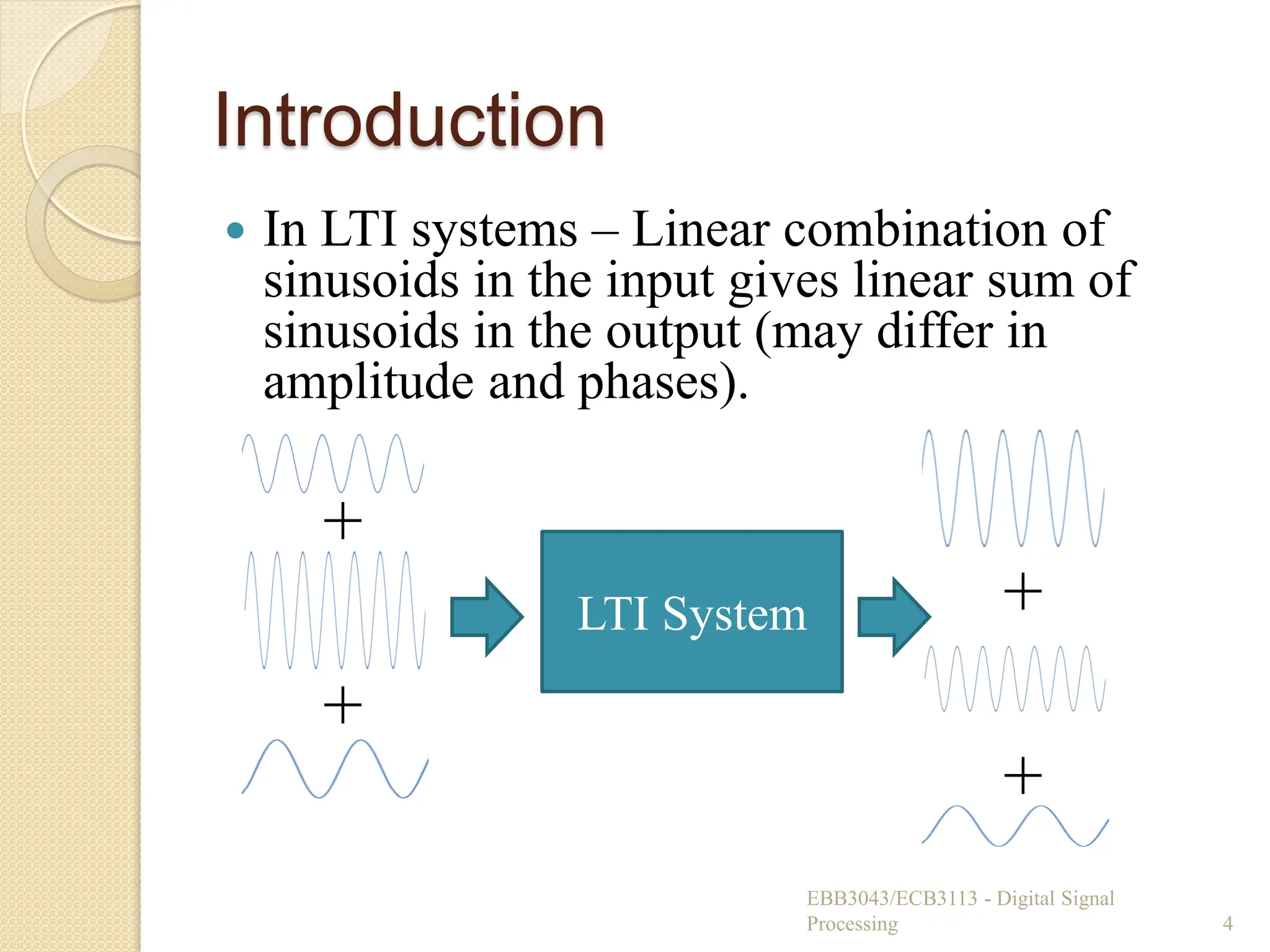
This document provides an overview of Fourier Analysis for Discrete-Time Linear Time-Invariant (LTI) systems. It explains how signals can be analyzed in the frequency domain using the Discrete-Time Fourier Transform (DTFT), focusing on concepts like magnitude and phase spectra. Key properties such as linearity, time-shifting, time-reversal, modulation, convolution, and Parseval’s theorem are covered. The document details the relationship between time-domain convolution and frequency-domain multiplication, introduces frequency response H(e^jω), and explains how to solve linear constant-coefficient difference equations (LCCDE) using DTFT. It concludes with the use of Inverse DTFT and common DTFT pairs for signal reconstruction and system analysis.

1. Topic 3
Fourier Analysis of Discrete Time LTI Systems
EBB3043/ECB3113 - Digital Signal
Processing 1

2. Introduction
 Most signals of practical interest can be
decomposed into a sum of sinusoidal
components.
EBB3043/ECB3113 - Digital Signal
Processing 2

3. Introduction
 In some cases, we
are more interested
in what the signal is
like in the frequency
domain, rather than
in the time-domain,
e.g. in an equalizer.
EBB3043/ECB3113 - Digital Signal
Processing 3

4. Introduction
 In LTI systems – Linear combination of
sinusoids in the input gives linear sum of
sinusoids in the output (may differ in
amplitude and phases).
EBB3043/ECB3113 - Digital Signal
Processing 4
LTI System
+
+
+
+

5. Sinusoid and sound
 A pure tone is a tone generated by a sinewave.
 In general, the frequency of a sinewave relates to
the pitch of a tone.
◦ The higher the frequency, the higher the pitch.
 The amplitude of a sinewave relates to the
loudness/strength of the tone.
◦ The higher the amplitude, the louder the sound.
 But, human hearing is limited e.g. if you hear two
pure tones of the same amplitude, but one is at a
low frequency and one is at a high frequency, the
one with low frequency may sound louder.
EBB3043/ECB3113 - Digital Signal
Processing 5

6. Try this…
 Run the following MATLAB code which generates a pure
tone with amplitude=0.1 and freq.=110Hz for 1 sec. Listen to
the sound.
 Create 2 other sinewaves:
◦ y2: amplitude = 0.1, frequency = 110 Hz
◦ y3: amplitude = 1, frequency = 880 Hz
 Compare:
◦ y1 and y2 – which sounds louder?
◦ y2 and y3 – which has the higher pitch?
 Does y1 sound louder than y3 even though they both have the
same amplitude?
EBB3043/ECB3113 - Digital Signal
Processing 6
y1=1*sin(2*pi*110/44100*[0:44099]);
sound(y1,44100)

7. Types of Fourier Analysis
 Signal is periodic and continuous –
Fourier series
 Signal is aperiodic and continuous –
Continuous-time Fourier transform (or
just Fourier Transform)
 Signal is aperiodic and discrete –
Discrete-time Fourier Transform (DTFT)
 Signal is periodic and discrete – Discrete
Fourier Transform (DFT)
EBB3043/ECB3113 - Digital Signal
Processing 7

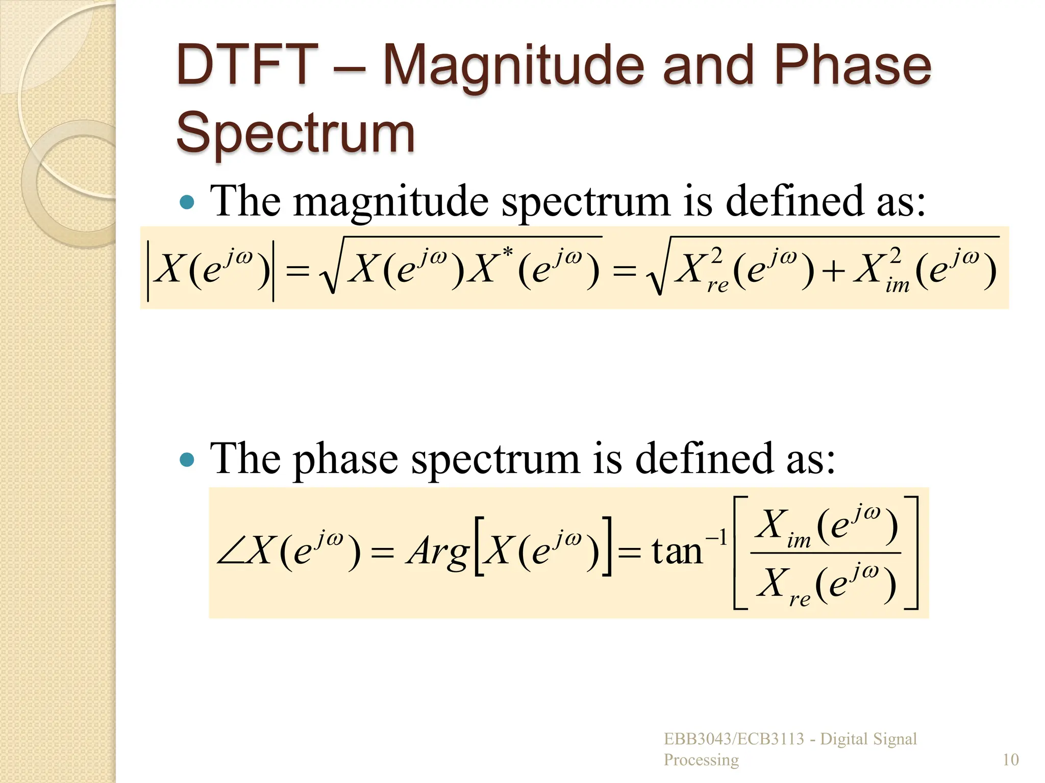
8. Discrete Time Fourier Transform
(DTFT)
 The DTFT of a sequence, x[n] is given as:
 The DTFT represents the frequency content
of x[n].
 The transformation can be represented by:
 X(ej) is also called the frequency spectrum
of the DT signal, x[n].
 The DTFT exists only for signals that are
absolutely summable i.e.
EBB3043/ECB3113 - Digital Signal
Processing 8






n
n
j
j
e
n
x
e
X 

]
[
)
(
.
]
[ 





n
n
x
)
(
]
[
)
(
]
[ 
 j
j
e
X
n
x
or
e
X
n
x 
 


 DTFT
F

9. DTFT – Magnitude and Phase
Spectrum
 The DTFT, X(ej), is complex-valued,  it
can be written in rectangular form:
X(ej) = Xre(ej)+j Xim(ej)
or polar form:
X(ej) =|X(ej)|X(ej)
EBB3043/ECB3113 - Digital Signal
Processing 9

10. )
(
)
(
)
(
)
(
)
( 2
2
* 



 j
im
j
re
j
j
j
e
X
e
X
e
X
e
X
e
X 


DTFT – Magnitude and Phase
Spectrum
 The magnitude spectrum is defined as:
 The phase spectrum is defined as:
EBB3043/ECB3113 - Digital Signal
Processing 10
  







 
)
(
)
(
tan
)
(
)
( 1




j
re
j
im
j
j
e
X
e
X
e
X
Arg
e
X

11. Properties of DTFT
 Linearity
◦ The DTFT of a linear weighted sum
combination of two signals is the linear
weighted sum of the DTFTs of the two signals.
 Periodicity
◦ The DTFT is periodic with period of 2,
where k is an integer.
EBB3043/ECB3113 - Digital Signal
Processing 11
)
(
)
(
]
[
]
[
)
(
]
[
)
(
]
[




j
j
j
j
e
bY
e
aX
n
by
n
ax
then
e
Y
n
y
and
e
X
n
x
If








F
F
F
)
(
)
( 2 

 j
k
j
e
X
e
X 


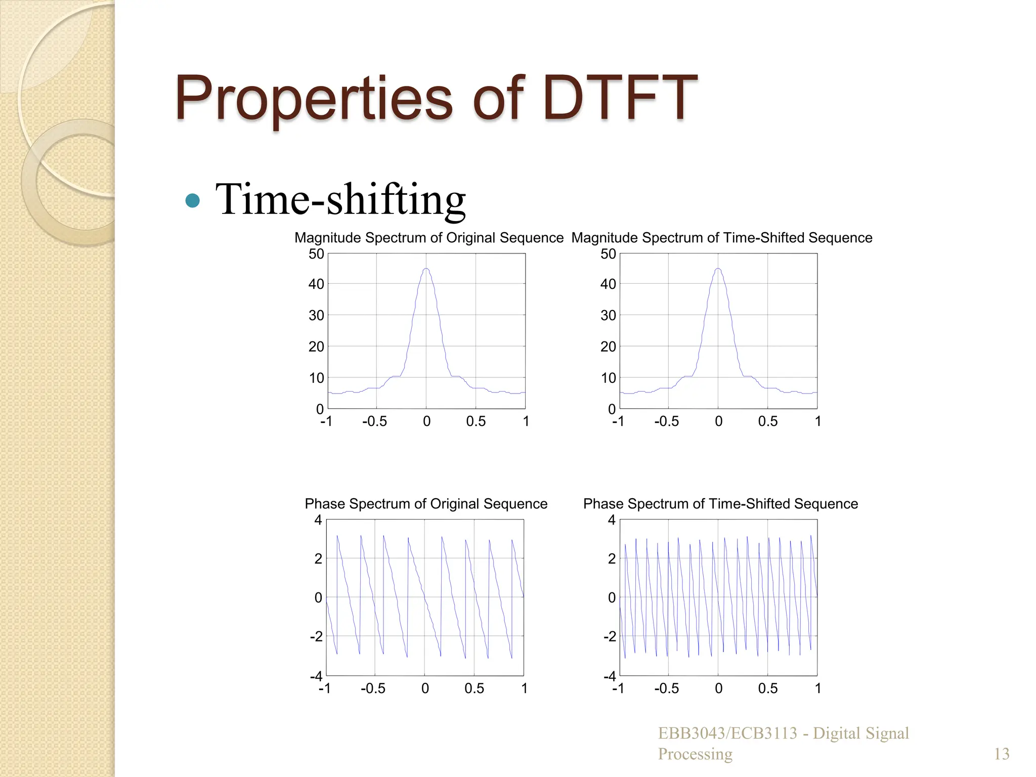
12. Properties of DTFT
 Time-shifting
◦ If signal is time-shifted by k samples, its
magnitude spectrum remains unchanged.
◦ The phase spectrum will change by amount -k.
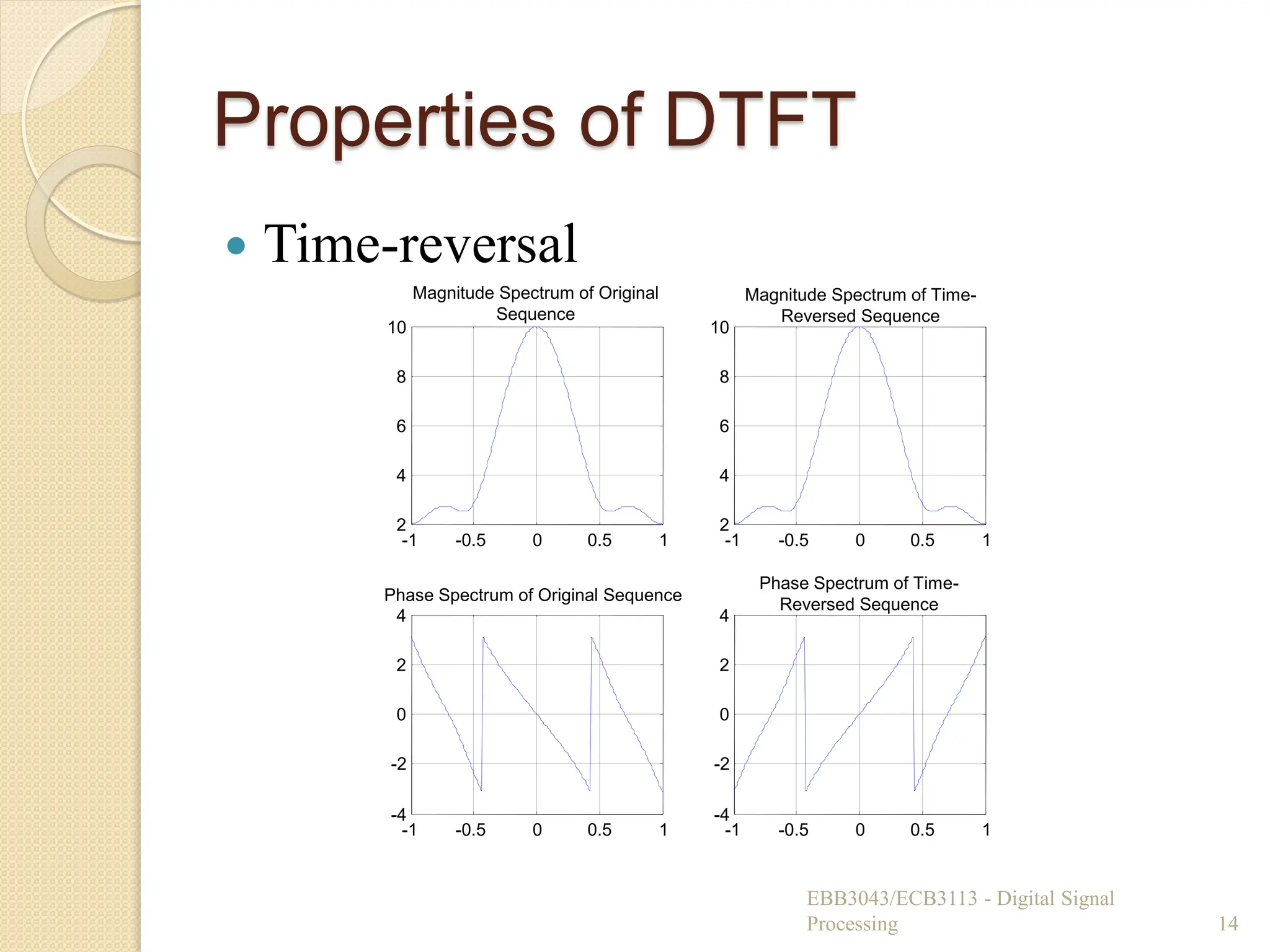
 Time-reversal
◦ If signal is folded about the origin in time, its
magnitude spectrum remains unchanged.
◦ Change in sign in the phase spectrum (Phase
reversal).
EBB3043/ECB3113 - Digital Signal
Processing 12
)
(
]
[
)
(
]
[ 

 j
k
j
j
e
X
e
k
n
x
then
e
X
n
x
If 




 F
F
)
(
]
[
)
(
]
[ 
 j
j
e
X
n
x
then
e
X
n
x
If 




 F
F

13. Properties of DTFT
 Time-shifting
EBB3043/ECB3113 - Digital Signal
Processing 13
-1 -0.5 0 0.5 1
0
10
20
30
40
50
Magnitude Spectrum of Original Sequence
-1 -0.5 0 0.5 1
0
10
20
30
40
50
Magnitude Spectrum of Time-Shifted Sequence
-1 -0.5 0 0.5 1
-4
-2
0
2
4
Phase Spectrum of Original Sequence
-1 -0.5 0 0.5 1
-4
-2
0
2
4
Phase Spectrum of Time-Shifted Sequence

14. Properties of DTFT
 Time-reversal
EBB3043/ECB3113 - Digital Signal
Processing 14
-1 -0.5 0 0.5 1
2
4
6
8
10
Magnitude Spectrum of Original
Sequence
-1 -0.5 0 0.5 1
2
4
6
8
10
Magnitude Spectrum of Time-
Reversed Sequence
-1 -0.5 0 0.5 1
-4
-2
0
2
4
Phase Spectrum of Original Sequence
-1 -0.5 0 0.5 1
-4
-2
0
2
4
Phase Spectrum of Time-
Reversed Sequence

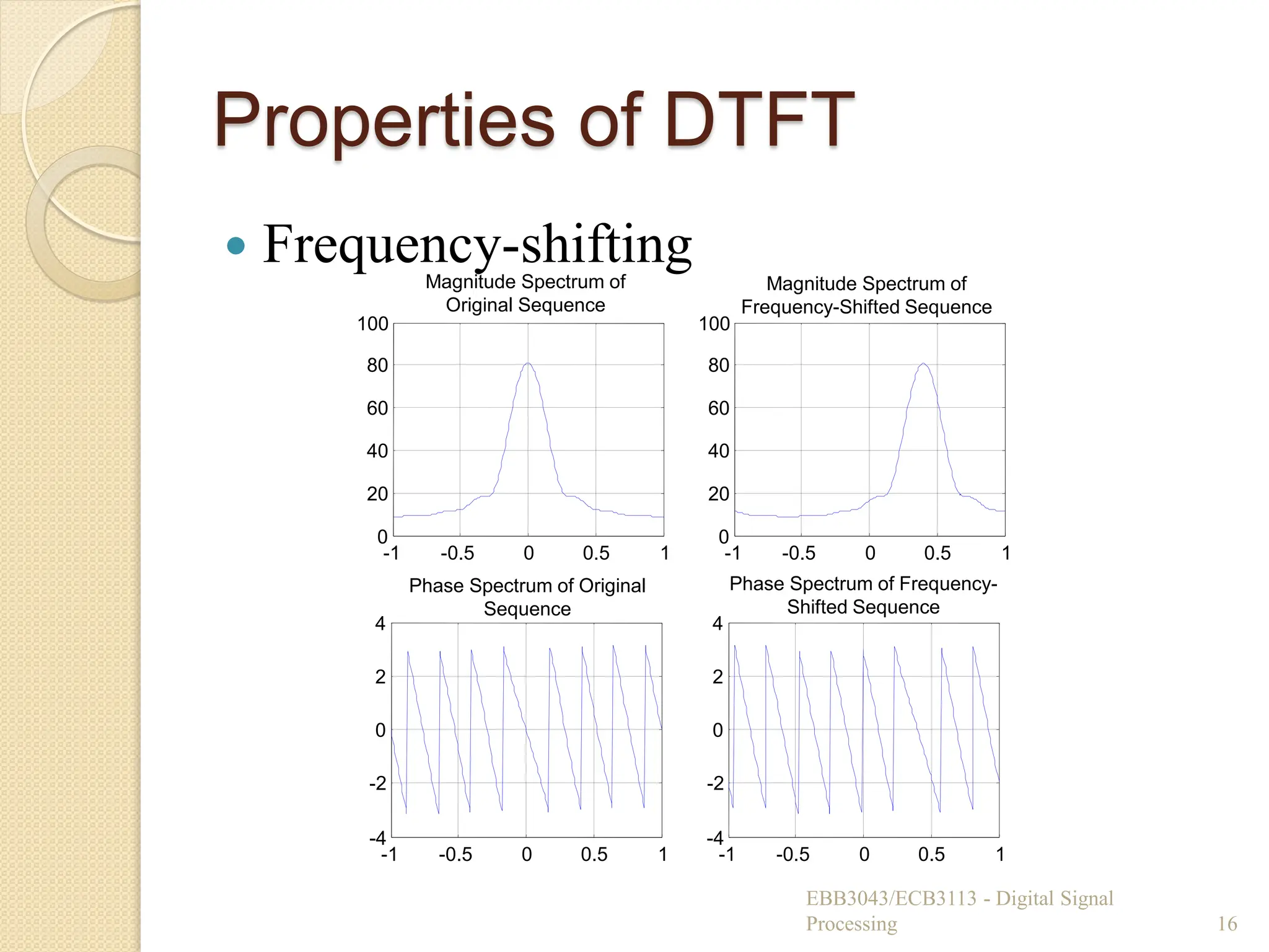
15. Properties of DTFT
 Frequency-shifting
◦ If signal is multiplied by , the spectrum is
shifted by 0.
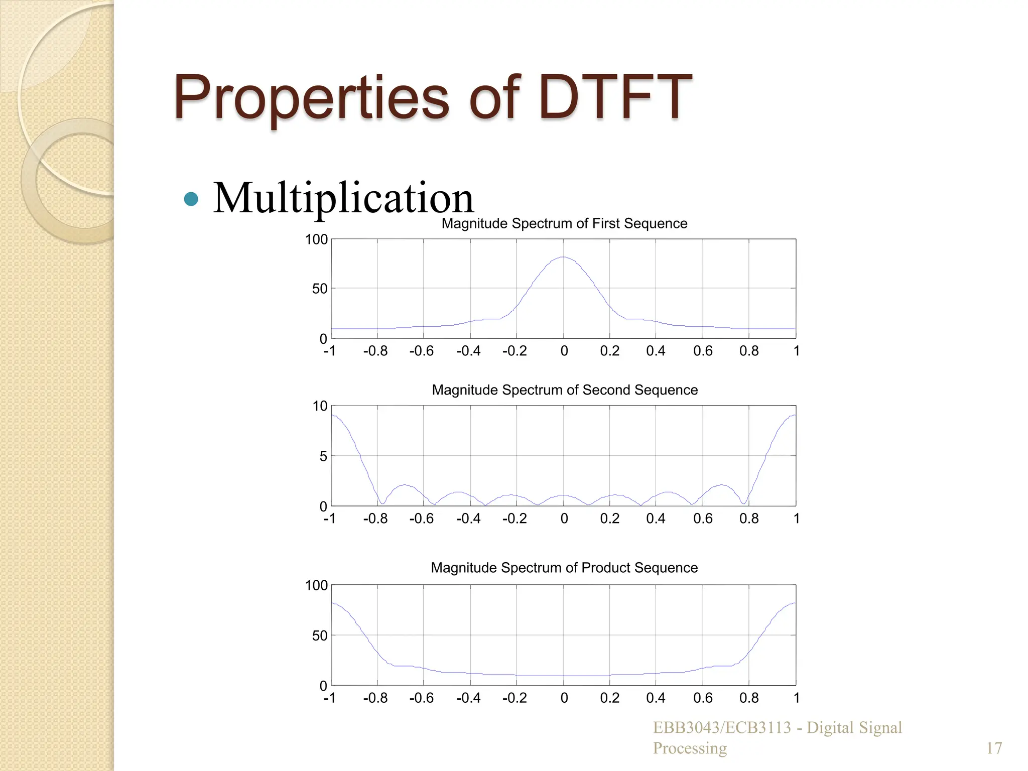
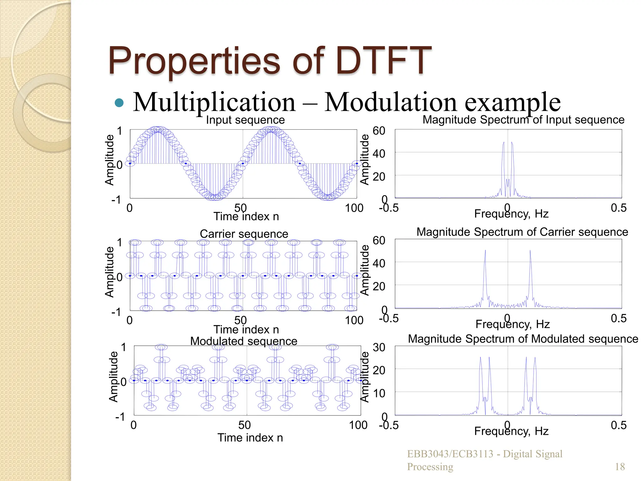
 Multiplication
◦ The DTFT of the product of two sequences is
the convolution of the individual DTFTs of the
two sequences.
EBB3043/ECB3113 - Digital Signal
Processing 15
)
(
]
[
)
(
]
[ )
( 0
0 


 




 j
n
j
j
e
X
n
x
e
then
e
X
n
x
If F
F
n
j
e 0


)
(
)
(
]
[
]
[
)
(
]
[
)
(
]
[




j
j
j
j
e
Y
e
X
n
y
n
x
then
e
Y
n
y
and
e
X
n
x
If







F
F
F

16. Properties of DTFT
 Frequency-shifting
EBB3043/ECB3113 - Digital Signal
Processing 16
-1 -0.5 0 0.5 1
0
20
40
60
80
100
Magnitude Spectrum of
Original Sequence
-1 -0.5 0 0.5 1
0
20
40
60
80
100
Magnitude Spectrum of
Frequency-Shifted Sequence
-1 -0.5 0 0.5 1
-4
-2
0
2
4
Phase Spectrum of Original
Sequence
-1 -0.5 0 0.5 1
-4
-2
0
2
4
Phase Spectrum of Frequency-
Shifted Sequence

17. Properties of DTFT
 Multiplication
EBB3043/ECB3113 - Digital Signal
Processing 17
-1 -0.8 -0.6 -0.4 -0.2 0 0.2 0.4 0.6 0.8 1
0
50
100
Magnitude Spectrum of First Sequence
-1 -0.8 -0.6 -0.4 -0.2 0 0.2 0.4 0.6 0.8 1
0
5
10
Magnitude Spectrum of Second Sequence
-1 -0.8 -0.6 -0.4 -0.2 0 0.2 0.4 0.6 0.8 1
0
50
100
Magnitude Spectrum of Product Sequence

18. Properties of DTFT
 Multiplication – Modulation example
EBB3043/ECB3113 - Digital Signal
Processing 18
Time index n
0 50 100
-1
0
1
Amplitude
Input sequence
Carrier sequence
0 50 100
-1
0
1
Amplitude
Time index n
0 50 100
-1
0
1
Time index n
Amplitude
Modulated sequence
-0.5 0 0.5
0
20
40
60
Frequency, Hz
Amplitude
Magnitude Spectrum of Input sequence
-0.5 0 0.5
0
20
40
60
Frequency, Hz
Amplitude
Magnitude Spectrum of Carrier sequence
-0.5 0 0.5
0
10
20
30
Frequency, Hz
Amplitude
Magnitude Spectrum of Modulated sequence

19. Properties of DTFT
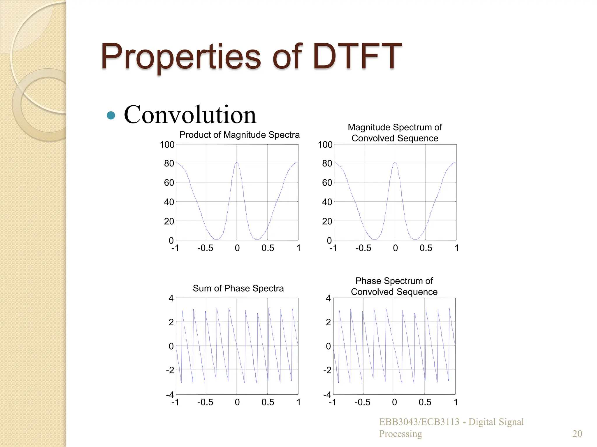
 Convolution
◦ If we convolve two sequences in the time-
domain, it is equivalent to multiplying their
DTFTs in the frequency domain.
EBB3043/ECB3113 - Digital Signal
Processing 19
)
(
)
(
]
[
]
[
)
(
]
[
)
(
]
[




j
j
j
j
e
Y
e
X
n
y
n
x
then
e
Y
n
y
and
e
X
n
x
If







F
F
F

20. Properties of DTFT
 Convolution
EBB3043/ECB3113 - Digital Signal
Processing 20
-1 -0.5 0 0.5 1
0
20
40
60
80
100
Product of Magnitude Spectra
-1 -0.5 0 0.5 1
0
20
40
60
80
100
Magnitude Spectrum of
Convolved Sequence
-1 -0.5 0 0.5 1
-4
-2
0
2
4
Sum of Phase Spectra
-1 -0.5 0 0.5 1
-4
-2
0
2
4
Phase Spectrum of
Convolved Sequence

21. Properties of DTFT
 Conjugation
 Differentiation
 Parseval’s Theorem
◦ Energy is conserved when going from the time
domain to the frequency domain.
EBB3043/ECB3113 - Digital Signal
Processing 21
)
(
]
[
)
(
]
[ 
 j
j
e
X
n
x
then
e
X
n
x
If 





 F
F
)
(
]
[
)
(
]
[ 


j
j
e
X
d
d
j
n
nx
then
e
X
n
x
If 


 F
F












d
e
X
n
x j
n
2
2
)
(
2
1
]
[

22. Common DTFT Pairs
EBB3043/ECB3113 - Digital Signal
Processing 22
)
2
(
)
2
(
cos
1
],
[
]
1
[
1
],
1
[
1
],
[
)
2
(
]
[
)
2
(
2
)
2
(
2
1
]
[
1
]
[
0
0
0
)
1
(
1
1
1
1
1
1
1
0
0
2
0
0
k
k
n
a
n
u
a
n
a
n
u
a
a
n
u
a
k
n
u
k
e
k
e
n
n
n
k
ae
n
ae
n
ae
n
k
e
k
jn
k
jn
j
j
j
j






































































Sequence DTFT

23. Inverse DTFT
 The IDTFT allows us to convert the
sequence from frequency domain to time
domain.
 The inverse DTFT is defined as:
 We can also represent the IDTFT as:
 Alternatively, we can use tables of DTFT
pairs to determine the IDTFT, or express ,
X(ej), as a power series of ej.
EDB2073- Digital Signal Processing © Nasreen Badruddin 23









d
e
e
X
n
x n
j
j
)
(
2
1
]
[
]
[
)
(
]
[
)
( n
x
e
X
or
n
x
e
X j
j

 


 IDTFT
F-1



24. Performing Convolution using
DTFT
 Convolution in the time domain is
equivalent to multiplication in the
frequency domain.
 To find the output of a system with
impulse response, h[n], when the input is
x[n], we do the following:
1. Find the DTFTs H(ej) and X(ej).
2. Perform the multiplication
Y (ej) =H(ej) X(ej).
3. Get the IDTFT of Y (ej) to obtain y[n].
EBB3043/ECB3113 - Digital Signal
Processing 24

25. The Frequency Response
 Recall that for an LTI system:
 Using the Convolution property of DTFT, we
have:
 H(ej) is called the frequency response of the
LTI system.
 It is the ratio of the DTFT of the output and
the DTFT of the input.
 It is also the DTFT of the impulse response.
EBB3043/ECB3113 - Digital Signal
Processing 25
]
[
]
[
]
[ n
h
n
x
n
y 

)
(
)
(
)
(
)
(
)
(
)
(
]
[
]
[
]
[






j
j
j
j
j
j
e
X
e
Y
e
H
e
H
e
X
e
Y
n
h
n
x
n
y






 F
)
(
]
[ 
j
e
H
n
h 
F

26. The Frequency Response
 The impulse response describes the
characteristics of the LTI system in the time
domain.
 Similarly, the frequency response describes
the characteristics of the LTI system in the
frequency domain.
 The drawback of the frequency response
using DTFT is that it is a continuous
function. Hence it cannot be processed by
digital systems.
 This problem is overcome by using the
Discrete Fourier Transform (DFT).
EBB3043/ECB3113 - Digital Signal
Processing 26

27. The Frequency Response
 H(ej) is a complex quantity. Hence it
produces a change in the magnitude and
phase of the input signal.
 The magnitude response is:
 The phase response is:
EBB3043/ECB3113 - Digital Signal
Processing 27
)
(
)
(
)
( 2
2 

 j
im
j
re
j
e
H
e
H
e
H 








 
)
(
)
(
tan
)
( 1



j
re
j
im
j
e
H
e
H
e
H

28. Solving LCCDE using DTFT
 Recall that the LCCDE has the general
form:
 Using linearity and shift properties of
DTFT, we can express the DE in the
frequency domain as:
EBB3043/ECB3113 - Digital Signal
Processing 28

 





N
k
k
M
k
k k
n
y
a
k
n
x
b
n
y
1
0
]
[
]
[
]
[
















N
k
j
k
j
k
M
k
j
k
j
k
j
N
k
k
M
k
k
e
Y
e
a
e
X
e
b
e
Y
k
n
y
a
k
n
x
b
n
y
1
0
1
0
)
(
)
(
)
(
]
[
]
[
]
[






29. Solving LCCDE using DTFT
 The DTFT can be used to solve LCCDE
to obtain the frequency response or the
impulse response.
 Steps:
1. Transform each term in the LCCDE into its
DTFT.
2. To get H(ej), manipulate the DTFT
equation to get the ratio Y(ej)/ X(ej).
3. To get h[n] perform IDTFT on H(ej).
EBB3043/ECB3113 - Digital Signal
Processing 29