1. Discrete-time systems
A system converts input to output:
E.g. Moving Average (MA):
x[n] DT System y[n]
(M = 3)
x[n]
y[n]
+
z-1
z-1
1/M
1/M
1/M
x[n-1]
x[n-2]
y[n]
1
M
x[n k]
602 - Digital Signal Processing, Semester VIII 10/31/2025 2
k
0
M 1
{y[n]} = f ({x[n]}) n
A
MA
Smoother
MA smoothesout rapid variations
(e.g. “12 month moving
average”)
e.g. signal noise
5 k
0
y[n] 1
4
x[n k]
5-pt
moving
average
x[n] = s[n] + d[n]
602 - Digital Signal Processing, Semester VIII 10/31/2025 4
4.
Accumulator
Output accumulatesall past inputs:
x[n] y[n]
+
z-1
602 - Digital Signal Processing, Semester VIII 10/31/2025 5
y[n-1]
n
y[n]
x[]
n
1
x[]
x[n]
y[n 1] x[n]
5.
Accumulator
n
x[n]
-1 1 23 4 5 6 7 8
9
A
y[n-1]
-1 1 2 3 4 5 6 7 8 9 n
1 2 3 4 5 6 7 8 9 n
y[n]
-1
x[n] y[n]
+
z-1
602 - Digital Signal Processing, Semester VIII 10/31/2025 6
y[n-1]
6.
Classes of DT
systems
Linear systems obey superposition:
if input x1[n] → output y1[n], x2 → y2 ...
given a linear combination
of inputs:
then output
for all , , x1 x2
i.e. same linear combination of outputs
x[n] DT system y[n]
602 - Digital Signal Processing, Semester VIII 10/31/2025 7
7.
Linearity: Example 1
Accumulator:
Linear
602 - Digital Signal Processing, Semester VIII 10/31/2025 8
n
y[n]
x[]
n
y[n] x1[]
x2[]
x1[]
x2[]
y1[n]
y2[n]
x[n] x1[n]
x2[n]
Linearity Example 3:
‘Offset’ accumulator:
but
Nonlinear
602 - Digital Signal Processing, Semester VIII 10/31/2025 10
.. unless C = 0
n
y[n] C
x[]
n
y1[n] C
x1[]
n
y[n] C x1[]
x2[]
y1[n]
y2[n]
10.
Property: Shift (time)invariance
602 - Digital Signal Processing, Semester VIII 10/31/2025 11
Time-shift of input
causes same shift in output
i.e. if x1[n] → y1[n]
then x[n] x1[n n0 ]
y[n] y1[n n0 ]
i.e. process doesn’t depend on absolute
value of n
11.
Shift-invariance counterexample
Upsampler:L
Not shift invariant
y[n] =
x[n/
L]
n = 0, ± L, ± 2L , . . .
0 otherwise
(n = r · L )
y1[n] = x1[n/L]
x[n] = x1[n - n0]
=} y[n] = x[n/L] = x1 [n/L - n0]
= x 1
n - L · n0
L
602 - Digital Signal Processing, Semester VIII 10/31/2025 12
= y1[n 0
- L · n ] = 1 0
/ y [n - n
]
x[n y[n]
{
12.
Another counterexample
Hence
If
then
Not shift invariant
- parameters depend on n
≠
y[n] n
x[n]
602 - Digital Signal Processing, Semester VIII 10/31/2025 13
scaling by time index
y1[n n0 ] n n0 x1[n n0 ]
x[n] x1[n n0 ]
y[n] n x1[n
n0 ]
13.
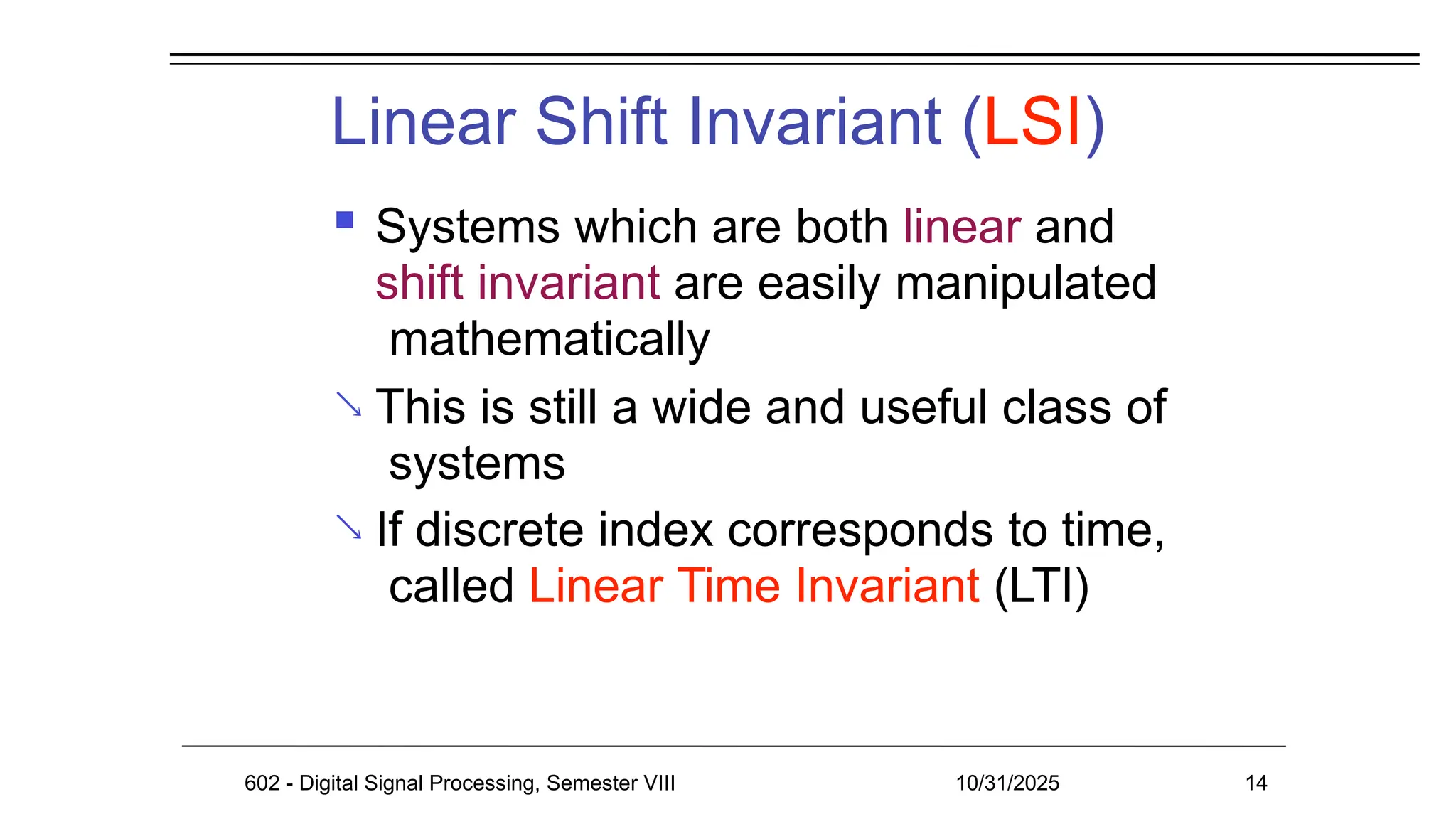
Linear Shift Invariant(LSI)
602 - Digital Signal Processing, Semester VIII 10/31/2025 14
Systems which are both linear and
shift invariant are easily manipulated
mathematically
This is still a wide and useful class of
systems
If discrete index corresponds to time,
called Linear Time Invariant (LTI)
14.
Causality
If outputdepends only on past and
current inputs (not future), system is
called causal
Formally, if x1[n] → y1[n] & x2[n] →
y2[n]
Causal x1[n] x2[n] n N
y1[n] y2[n]
n N
602 - Digital Signal Processing, Semester VIII 10/31/2025 15
15.
Causality example
Movingaverage:
y[n]
y[n] depends on x[n-k], k ≥ 0 → causal
‘Centered’ moving average
.. looks forward in time → noncausal
.. Can make causal by delaying
1
M
x[n k]
k
0
M 1
c
y n yn M 1 /
2
1
M
x[n]
602 - Digital Signal Processing, Semester VIII 10/31/2025 16
x[n k] x[n k]
(M 1) /
2
k 1
16.
602 - DigitalSignal Processing, Semester VIII 10/31/2025 17
17.
Impulse response (IR)
Impulse
(unit sample sequence)
Given a system:
if x[n] = [n] then
“impulse response”
LSI system completely specified by h[n]
n
1 2 3 4 5 6
7
[n] 1
-3 -2 -1
x[n] DT system y[n]
602 - Digital Signal Processing, Semester VIII 10/31/2025 18
Y[n]
18.
Impulse response example
Simple system:
α
x[n]
y[n]
+
z-1
z-1
α2
α3
n
1 2 3 4 5 6
7
x[n] 1
-3 -2 -1
n
y[n]
1 2 3 4 5 6
7
α
-3 -2 -1
α
α
x[n] [n] impulse
y[n] = h[n] impulse response
602 - Digital Signal Processing, Semester VIII 10/31/2025 19
19.
2. Convolution
Impulseresponse:
Shift invariance:
+ Linearity:
Can express any sequence with s:
x[n] = x[0][n] + x[1][n-1] + x[2][n-
2]..
[n]
LSI h[n]
[n-
n0]
LSI h[n-n0]
α·[n-k]
+ β·[n-l]
LSI
α·h[n-k]
+ β·h[n-l]
602 - Digital Signal Processing, Semester VIII 10/31/2025 20
20.
602 - DigitalSignal Processing, Semester VIII 10/31/2025 21
21.
602 - DigitalSignal Processing, Semester VIII 10/31/2025 22
22.
Convolution
sum
Hence, since
Convolution
sum
x[n] x[k][n
k]
k
k
For LSI, y[n] x[k]h[n
k]
written as y[n] x[n] * h[n]
Summation is symmetric in x and h
i.e. l = n – k →
l
x[n] * h[n] x[n l]h[l] h[n] * x[n]
602 - Digital Signal Processing, Semester VIII 10/31/2025 23
Interpreting convolution
Passinga signal through a (LSI) system
is equivalent to convolving it with the
system’s impulse response
x[n] h[n] y[n] = x[n] ∗
h[n]
x[n]={0 3 1 2 -1} h[n] = {3 2 1}
n
1 2 3 4 5 6
7
-3 -2 -1
n
1 2
3
5 6
7
-3 -2 -1
y[n] x[k]h[n k]
h[k]x[n k]
k k
602 - Digital Signal Processing, Semester VIII 10/31/2025 25
→
→
25.
Convolution interpretation 1
Time-reverse h,
shift by n, take inner
product against
fixed x
k
1 2 3 5 6
7
-3 -2 -1
x[k]
k
1 2 3 4 5 6
7
-3 -2 -1
h[0-k]
k
1 2 3 4 5 6
7
-3 -2 -1
k
1 2 3 4 5 6
7
-3 -2 -1
h[2-k]
n
1 2
3
5 7
-3 -2 -1
y[n]
0
9 9
11
2
-1
k
602 - Digital Signal Processing, Semester VIII 10/31/2025 26
y[n] x[k]h[n
k]
=g[k]
h[1-k]
=g[k-1]
call h[-n] = g[n]
26.
Convolution interpretation 2
Shifted x’s
weighted by
points in h
Conversely,
weighted,
delayed
versions of h ...
n
1 2
3
5 7
-3 -2 -1
y[n]
0
9 9
11
2
-1
n
1 2
3
5 6
7
-3 -2 -1
x[n]
n
1 2 3
4
6
7
-3 -2 -1
x[n-1]
n
1 2 3 4
5
7
-3 -2 -1
x[n-2]
k
1
2
3
4
5
6
7
h[k]
-3
-2
-1
602 - Digital Signal Processing, Semester VIII 10/31/2025 27
y[n] h[k]x[n k]
k
27.
Matrix interpretation
602 -Digital Signal Processing, Semester VIII 10/31/2025 28
Diagonals in X matrix are equal
𝑦 [𝑛]= ∑
𝑘=− ∞
∞
𝑥 [𝑛−𝑘]h[𝑘]
[
𝑦 [ 0 ]
𝑦 [ 1 ]
𝑦 [ 2 ]
⋯
]= ¿
28.
Convolution
notes
602 - DigitalSignal Processing, Semester VIII 10/31/2025 29
Total nonzero length of convolving N
and M point sequences is N+M-1
Adding the indices of the terms within
the summation gives n :
k
i.e. summation indices move in opposite
senses
y[n] h[k]x[n k]
k
n k n
29.
Convolution in MATLAB
602- Digital Signal Processing, Semester VIII 10/31/2025 30
The M-file conv implements the
convolution sum of two finite-length
sequences
If a
[0
b
[3
3 1 2 -1]
2 1]
then conv(a,b) yields
[0 9 9 11 2 0 -1]
30.
Connected
systems
Cascade connection:
Impulseresponse h[n] of the cascade of
two systems with impulse responses
h1[n] and h2[n] is
By commutativity,
*
h[n] h1[n]⊛
602 - Digital Signal Processing, Semester VIII 10/31/2025 31
31.
602 - DigitalSignal Processing, Semester VIII 10/31/2025 32
32.
Inverse systems
[n] is identity for convolution
i.e. x[n] * [n] x[n]
Consider
x[n]
y[n]
z[n]
z[n] h2 [n] * y[n] h2 [n] * h1[n] *
x[n]
x[n] if h2[n] * h1[n] [n]
602 - Digital Signal Processing, Semester VIII 10/31/2025 33
33.
Inverse systems
Useinverse system to recover input x[n]
from output y[n] (e.g. to undo effects of
transmission channel)
Only sometimes possible - e.g. cannot
‘invert’ h1[n] = 0
In general, attempt to solve
h2[n] * h1[n] [n]
602 - Digital Signal Processing, Semester VIII 10/31/2025 34
34.
Inverse system example
Accumulator:
Impulse response h1[n] = μ[n]
Thus, ‘backwards difference’ is inverse
system of accumulator.
‘Backwards difference’
.. has desired property:
[n] [n 1] [n]
n
-3 -2 -1 1 2 3 4 5 6
7
n
-3 -2 -1 1 2 3 4 5 6
7
602 - Digital Signal Processing, Semester VIII 10/31/2025 35
35.
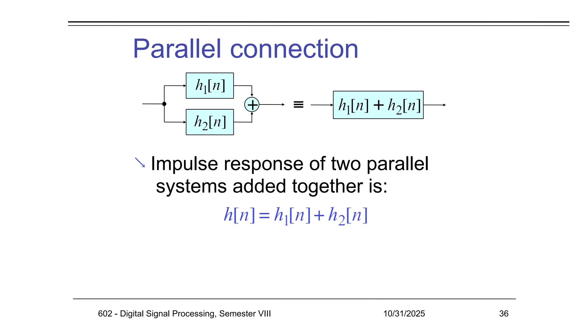
Parallel connection
Impulseresponse of two parallel
systems added together is:
602 - Digital Signal Processing, Semester VIII 10/31/2025 36
36.
3. Linear Constant-Coefficient
DifferenceEquation(LCCDE)
General spec. of DT, LSI, finite-dim sys:
Rearrange for y[n] in causal form:
WLOG, always have d0 = 1
defined by {dk},{pk}
order = max(N,M)
k0 k0
N M
dk y[n k] pk x[n k]
k
y[n]
d
p
k
k1 d0 k0 d0
602 - Digital Signal Processing, Semester VIII 10/31/2025 37
N M
y[n k]
x[n k]
37.
602 - DigitalSignal Processing, Semester VIII 10/31/2025 38
38.
Solving
LCCDEs
“Total solution”
y[n]yc[n] yp [n]
Complementary Solution
N
satisfies
Particular Solution
for given forcing function
x[n]
602 - Digital Signal Processing, Semester VIII 10/31/2025 39
dk y [n k] 0
k0
39.
Complementary Solution
602 -Digital Signal Processing, Semester VIII 10/31/2025 40
General form of unforced oscillation
i.e. system’s ‘natural modes’
Characteristic polynomial
of system - depends only on {dk}
yc [n]
n
k
d
nk
k0
Assume yc has form
N
0
nN
0
N
1
d d N 1
... d N 1 N
d 0
k
d
N k
N
k0
0
40.
Complementary Solution
602 -Digital Signal Processing, Semester VIII 10/31/2025 41
i
factors into roots λ , i.e.
Each/any λi satisfies eqn.
Thus, complementary solution:
Any linear combination will work
→ αis are free to match initial conditions
k
d
N k
N
k0
0
1 2
( )(
)... 0
y [n]
c 1 1 2 2 3 3
n n n
...
41.
Complementary Solution
Repeatedroots in chr. poly:
n
y [n]
c 1 1
n n
n2
n
2 1 3
1
... nL1
n
...
L
1
1 2
n
( )L
( )... 0
602 - Digital Signal Processing, Semester VIII 10/31/2025 42
42.
Particular Solution
602 -Digital Signal Processing, Semester VIII 10/31/2025 43
Recall: Total solution
Particular solution reflects input
‘Modes’ usually decay away for large n
leaving just yp[n]
Assume ‘form’ of x[n], scaled by β:
e.g. x[n] constant → yp[n] = β
x[n] = λ → y [n] = β · λ
0 p 0
n n (λ0 ∉
λi)
or = β nL λ0
n (λ0 ∈
λi)
y[n] yc[n] yp [n]
43.
LCCDE
example
Need input:x[n] =
8μ[n]
Need initial conditions:
y[-1] = 1, y[-2] = -1
y[n] y[n 1] 6y[n 2] x[n]
x[n] + y[n]
602 - Digital Signal Processing, Semester VIII 10/31/2025 44
44.
LCCDE example
602 -Digital Signal Processing, Semester VIII 10/31/2025 45
Complementary solution:
y[n] y[n 1] 6y[n 2] 0;
3 2 0 →roots λ = -3, λ =
2
1 2
yc [n] 1 3 2 2
n n
α1, α2 are unknown at this point
y[n]
n
n2
2
6 0
Solve forunknown αis by substituting
n = 0
LCCDE
example
from ICs
initial conditions into DE at n = 0, 1, ...
y[n] y[n 1] 6y[n 2] x[n]
602 - Digital Signal Processing, Semester VIII 10/31/2025 47
1 2
n n
3 2
Total solution y[n] yc[n] yp
[n]
y[0] y[1] 6y[2] x[0]
1 6 8
1 2
3
1 2
47.
LCCDE
example
n =1
Don’t find αis by solving with ICs at
n = -1,-2
(ICs may not reflect natural modes;
Mitra3 ex 2.37-8 (4.22-3) is
wrong)
602 - Digital Signal Processing, Semester VIII 10/31/2025 48
y[1] y[0] 6y[1] x[1]
(3) (2)
6 8
1 2 1 2
1 2
2 3 18
solve: α1 = -1.8, α2 = 4.8
Hence, system output:
y[n] 1.8(3)n
4.8(2)n
2 n
0
48.
LCCDE solving
summary
602 -Digital Signal Processing, Semester VIII 10/31/2025 49
Difference Equation (DE):
Ay[n] + By[n-1] + ... = Cx[n] + Dx[n-1] + ...
Initial Conditions (ICs): y[-1] = ...
DE RHS = 0 with y[n]=λn → roots {λi}
gives complementary soln
Particular soln: yp[n] ~
x[n]
solve for βλ0
n “at large n”
αis by substituting DE at n = 0, 1, ...
ICs for y[-1], y[-2]; yt=yc+yp for y[0], y[1]
c
y [n]
i i
n
49.
LCCDEs: zero input/zerostate
602 - Digital Signal Processing, Semester VIII 10/31/2025 50
Alternative approach to solving
LCCDEs is to solve two subproblems:
yzi[n], response with zero input (just ICs)
yzs[n], response with zero state (just x[n])
Because of linearity, y[n] = yzi[n]+yzs[n]
Both subproblems are ‘fully realized’
But, have to solve for αis twice
(then sum them)
50.
Impulse response ofLCCDEs
Impulse response:
i.e. solve with x[n] = δ[n] → y[n] = h[n]
(zero ICs)
With x[n] = δ[n], ‘form’ of yp[n] = βδ[n]
→ solve y[n] for n = 0,1, 2... to find αis
δ[n] LCCDE h[n]
602 - Digital Signal Processing, Semester VIII 10/31/2025 51
51.
LCCDE IR
example
thus
1
602- Digital Signal Processing, Semester VIII 10/31/2025 52
n ≥ 0
Infinite length
e.g. y[n] y[n 1] 6y[n 2] x[n]
(from before); x[n] = δ[n]; y[n] = 0 for n<0
y [n]
c 1 2
3 2
n n
h[n] 0.63
n
0.42
n
yp[n] = βδ[n]
n = 0: y[0] y[1] 6y[2] x[0]
α1 + α2 + β = 1
n = 1: α1(–3) + α2(2) + 1 = 0
n = 2: α1(9) + α2(4) – 1 – 6 = 0
α1 = 0.6, α2 = 0.4, β = 0
52.
System property: Stability
Outputgrows without limit in some
conditions
z-1
2
n
Certain systems can be unstable e.g.
x[n] + y[n] y[n]
-1 1 2 3
4
...
602 - Digital Signal Processing, Semester VIII 10/31/2025 53
53.
Stability
Several definitionsfor stability; we use
Bounded-input, bounded-output
(BIBO) stable
For every bounded input x[n]
Bx
n
output is also subject to a finite bound,
y[n] By n
602 - Digital Signal Processing, Semester VIII 10/31/2025 54
54.
Stability example
MA
filter:
→BIBO Stable
M k0
y[n] 1
M 1
x[n k]
M k0
y[n] 1
M 1
x[n k]
M k0
1
M 1
x[n k]
M
1
M B
B
602 - Digital Signal Processing, Semester VIII 10/31/2025 55
x y
55.
Stability &
LCCDEs
602 -Digital Signal Processing, Semester VIII 10/31/2025 56
LCCDE output is of form:
y[n] n
n
...
n
1 1 2
2 0
αs and βs depend on input & ICs,
but to be bounded for any input
we need |λ
...
56.
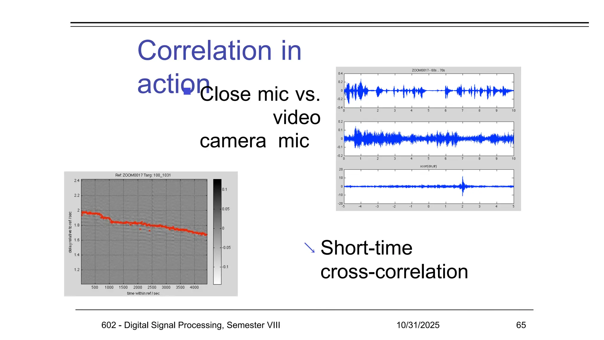
4. Correlation
Correlation~ identifies similarity
between sequences:
Cross
of x against y
“lag”
correlation
602 - Digital Signal Processing, Semester VIII 10/31/2025 57
𝑟 𝑥𝑦 [𝑙 ]= ∑
𝑛=− ∞
∞
𝑥 [ 𝑛 ] 𝑦 [𝑛 − 𝑙]
Note: 𝑟 𝑦𝑥 [𝑙]= ∑
𝑛=− ∞
∞
𝑦 [𝑛] 𝑥[𝑛−𝑙]
Set m = n-l
57.
Correlation and convolution
602- Digital Signal Processing, Semester VIII 10/31/2025 58
Correlation:
Convolution:
Hence:
Correlation may be calculated by
convolving with time-reversed sequence
𝑟𝑥𝑦 [𝑛]= ∑
𝑘=−∞
∞
𝑥[𝑘] 𝑦[𝑘−𝑛]
𝑥[𝑛]⊛𝑦 [𝑛]= ∑
𝑘=−∞
∞
𝑥[𝑘]𝑦 [𝑛−𝑘]
𝑟 𝑥𝑦 [𝑛]=𝑥[𝑛]⊛ 𝑦[−𝑛]
58.
Autocorrelation
602 - DigitalSignal Processing, Semester VIII 10/31/2025 59
Energy of
sequence x[n]
xx
Note: r [0]
2
n
x [n]
x
Autocorrelation (AC) is correlation of
signal with itself:
𝑟𝑥𝑥[𝑙]= ∑
𝑛=−∞
∞
𝑥 [𝑛]𝑥 [𝑛−𝑙]=𝑟𝑥𝑥[−𝑙]
59.
Correlation
maxima
Note:
Fromgeometry,
when x//y, cosθ = 1, else cosθ <
1
angle
between
x and y
rxx [] rxx [0]
rxx
[]
rxx [0]
1
xy
Similarly: r []
x y
rxy
[]
rxx [0]ryy
[0]
1
i
xy xi yi x y
cos
xi
2
602 - Digital Signal Processing, Semester VIII 10/31/2025 60
60.
AC of aperiodic
sequence
Sequence of period N: x˜[n] x˜[n
N ]
Calculate AC over a finite window:
if M >> N
rx˜x˜
[]
1
2M 1 n M
M
x˜[n]x˜[n
]
1
N n0
N 1
602 - Digital Signal Processing, Semester VIII 10/31/2025 61
x˜[n]x˜[n
]
61.
AC of aperiodic
sequence
i.e AC of periodic sequence is
periodic
Average energy per
sample or Power of x
x˜
x˜
r [0]
1
N
2
x˜[n] P
N 1
n0
x
˜
rx˜x˜ [ N ]
1
N n0
N 1
602 - Digital Signal Processing, Semester VIII 10/31/2025 62
x˜[n]x˜[n N ] rx˜x˜
[]
62.
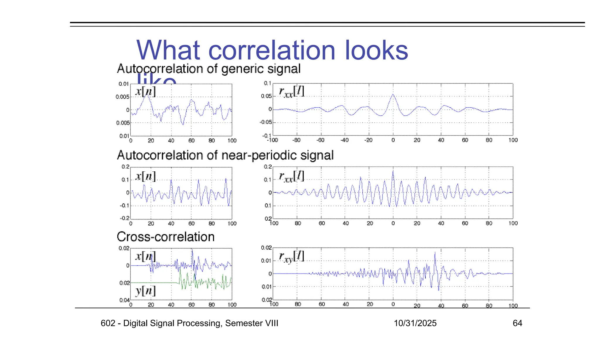
Cross correlation
rxy[]
What correlations look like
AC of any x[n]
AC of periodic
rxx
[]
602 - Digital Signal Processing, Semester VIII 10/31/2025 63
rx˜x˜ []
![1. Discrete-time systems
A system converts input to output:
E.g. Moving Average (MA):
x[n] DT System y[n]
(M = 3)
x[n]
y[n]
+
z-1
z-1
1/M
1/M
1/M
x[n-1]
x[n-2]
y[n]
1
M
x[n k]
602 - Digital Signal Processing, Semester VIII 10/31/2025 2
k
0
M 1
{y[n]} = f ({x[n]}) n
A](https://image.slidesharecdn.com/l02-timedom-251031042137-3c246787/75/Time-domain-representation-of-signals-and-systems-1-2048.jpg)
![Moving Average
(MA)
x[n]
y[n]
+
z-1
z-1
1/M
1/M
1/M
x[n-1]
x[n-2]
n
x[n]
1 2 3 4 5 6 7 8
9
A
n
-1
x[n-
1]
1 2 3 4 5 6 7 8
9
-1
x[n-
2]
-1 1 2 3 4 5 6 7 8 9 n
1 2 3 4 5 6 7 8 9 n
y[n]
-1
y[n]
1
M
x[n k]
602 - Digital Signal Processing, Semester VIII 10/31/2025 3
k
0
M 1
](https://image.slidesharecdn.com/l02-timedom-251031042137-3c246787/75/Time-domain-representation-of-signals-and-systems-2-2048.jpg)
![MA
Smoother
MA smoothes out rapid variations
(e.g. “12 month moving
average”)
e.g. signal noise
5 k
0
y[n] 1
4
x[n k]
5-pt
moving
average
x[n] = s[n] + d[n]
602 - Digital Signal Processing, Semester VIII 10/31/2025 4](https://image.slidesharecdn.com/l02-timedom-251031042137-3c246787/75/Time-domain-representation-of-signals-and-systems-3-2048.jpg)
![Accumulator
Output accumulates all past inputs:
x[n] y[n]
+
z-1
602 - Digital Signal Processing, Semester VIII 10/31/2025 5
y[n-1]
n
y[n]
x[]
n
1
x[]
x[n]
y[n 1] x[n]](https://image.slidesharecdn.com/l02-timedom-251031042137-3c246787/75/Time-domain-representation-of-signals-and-systems-4-2048.jpg)
![Accumulator
n
x[n]
-1 1 2 3 4 5 6 7 8
9
A
y[n-1]
-1 1 2 3 4 5 6 7 8 9 n
1 2 3 4 5 6 7 8 9 n
y[n]
-1
x[n] y[n]
+
z-1
602 - Digital Signal Processing, Semester VIII 10/31/2025 6
y[n-1]](https://image.slidesharecdn.com/l02-timedom-251031042137-3c246787/75/Time-domain-representation-of-signals-and-systems-5-2048.jpg)
![Classes of DT
systems
Linear systems obey superposition:
if input x1[n] → output y1[n], x2 → y2 ...
given a linear combination
of inputs:
then output
for all , , x1 x2
i.e. same linear combination of outputs
x[n] DT system y[n]
602 - Digital Signal Processing, Semester VIII 10/31/2025 7](https://image.slidesharecdn.com/l02-timedom-251031042137-3c246787/75/Time-domain-representation-of-signals-and-systems-6-2048.jpg)
![Linearity: Example 1
Accumulator:
Linear
602 - Digital Signal Processing, Semester VIII 10/31/2025 8
n
y[n]
x[]
n
y[n] x1[]
x2[]
x1[]
x2[]
y1[n]
y2[n]
x[n] x1[n]
x2[n]](https://image.slidesharecdn.com/l02-timedom-251031042137-3c246787/75/Time-domain-representation-of-signals-and-systems-7-2048.jpg)
![Linearity Example 2:
“Teager Energy operator”:
y[n] x2
[n] x[n 1] x[n
1]
x[n] x1[n] x2[n]
Nonlinear
602 - Digital Signal Processing, Semester VIII 10/31/2025 9
y[n]
1
2
x [n] x
[n]
2
x1[n 1] x2[n 1]
x1[n 1]
x2[n 1]
y1[n]
y2[n]](https://image.slidesharecdn.com/l02-timedom-251031042137-3c246787/75/Time-domain-representation-of-signals-and-systems-8-2048.jpg)
![Linearity Example 3:
‘Offset’ accumulator:
but
Nonlinear
602 - Digital Signal Processing, Semester VIII 10/31/2025 10
.. unless C = 0
n
y[n] C
x[]
n
y1[n] C
x1[]
n
y[n] C x1[]
x2[]
y1[n]
y2[n]](https://image.slidesharecdn.com/l02-timedom-251031042137-3c246787/75/Time-domain-representation-of-signals-and-systems-9-2048.jpg)
![Property: Shift (time) invariance
602 - Digital Signal Processing, Semester VIII 10/31/2025 11
Time-shift of input
causes same shift in output
i.e. if x1[n] → y1[n]
then x[n] x1[n n0 ]
y[n] y1[n n0 ]
i.e. process doesn’t depend on absolute
value of n](https://image.slidesharecdn.com/l02-timedom-251031042137-3c246787/75/Time-domain-representation-of-signals-and-systems-10-2048.jpg)
![Shift-invariance counterexample
Upsampler: L
Not shift invariant
y[n] =
x[n/
L]
n = 0, ± L, ± 2L , . . .
0 otherwise
(n = r · L )
y1[n] = x1[n/L]
x[n] = x1[n - n0]
=} y[n] = x[n/L] = x1 [n/L - n0]
= x 1
n - L · n0
L
602 - Digital Signal Processing, Semester VIII 10/31/2025 12
= y1[n 0
- L · n ] = 1 0
/ y [n - n
]
x[n y[n]
{](https://image.slidesharecdn.com/l02-timedom-251031042137-3c246787/75/Time-domain-representation-of-signals-and-systems-11-2048.jpg)
![Another counterexample
Hence
If
then
Not shift invariant
- parameters depend on n
≠
y[n] n
x[n]
602 - Digital Signal Processing, Semester VIII 10/31/2025 13
scaling by time index
y1[n n0 ] n n0 x1[n n0 ]
x[n] x1[n n0 ]
y[n] n x1[n
n0 ]](https://image.slidesharecdn.com/l02-timedom-251031042137-3c246787/75/Time-domain-representation-of-signals-and-systems-12-2048.jpg)
![Causality
If output depends only on past and
current inputs (not future), system is
called causal
Formally, if x1[n] → y1[n] & x2[n] →
y2[n]
Causal x1[n] x2[n] n N
y1[n] y2[n]
n N
602 - Digital Signal Processing, Semester VIII 10/31/2025 15](https://image.slidesharecdn.com/l02-timedom-251031042137-3c246787/75/Time-domain-representation-of-signals-and-systems-14-2048.jpg)
![Causality example
Moving average:
y[n]
y[n] depends on x[n-k], k ≥ 0 → causal
‘Centered’ moving average
.. looks forward in time → noncausal
.. Can make causal by delaying
1
M
x[n k]
k
0
M 1
c
y n yn M 1 /
2
1
M
x[n]
602 - Digital Signal Processing, Semester VIII 10/31/2025 16
x[n k] x[n k]
(M 1) /
2
k 1
](https://image.slidesharecdn.com/l02-timedom-251031042137-3c246787/75/Time-domain-representation-of-signals-and-systems-15-2048.jpg)

![Impulse response (IR)
Impulse
(unit sample sequence)
Given a system:
if x[n] = [n] then
“impulse response”
LSI system completely specified by h[n]
n
1 2 3 4 5 6
7
[n] 1
-3 -2 -1
x[n] DT system y[n]
602 - Digital Signal Processing, Semester VIII 10/31/2025 18
Y[n]](https://image.slidesharecdn.com/l02-timedom-251031042137-3c246787/75/Time-domain-representation-of-signals-and-systems-17-2048.jpg)
![Impulse response example
Simple system:
α
x[n]
y[n]
+
z-1
z-1
α2
α3
n
1 2 3 4 5 6
7
x[n] 1
-3 -2 -1
n
y[n]
1 2 3 4 5 6
7
α
-3 -2 -1
α
α
x[n] [n] impulse
y[n] = h[n] impulse response
602 - Digital Signal Processing, Semester VIII 10/31/2025 19](https://image.slidesharecdn.com/l02-timedom-251031042137-3c246787/75/Time-domain-representation-of-signals-and-systems-18-2048.jpg)
![2. Convolution
Impulse response:
Shift invariance:
+ Linearity:
Can express any sequence with s:
x[n] = x[0][n] + x[1][n-1] + x[2][n-
2]..
[n]
LSI h[n]
[n-
n0]
LSI h[n-n0]
α·[n-k]
+ β·[n-l]
LSI
α·h[n-k]
+ β·h[n-l]
602 - Digital Signal Processing, Semester VIII 10/31/2025 20](https://image.slidesharecdn.com/l02-timedom-251031042137-3c246787/75/Time-domain-representation-of-signals-and-systems-19-2048.jpg)


![Convolution
sum
Hence, since
Convolution
sum
x[n] x[k][n
k]
k
k
For LSI, y[n] x[k]h[n
k]
written as y[n] x[n] * h[n]
Summation is symmetric in x and h
i.e. l = n – k →
l
x[n] * h[n] x[n l]h[l] h[n] * x[n]
602 - Digital Signal Processing, Semester VIII 10/31/2025 23](https://image.slidesharecdn.com/l02-timedom-251031042137-3c246787/75/Time-domain-representation-of-signals-and-systems-22-2048.jpg)
![Convolution properties
LSI System output y[n] = input x[n]
convolved with impulse response h[n]
→ h[n] completely describes system
Commutative: x[n] * h[n] = h[n] * x[n]
Associative:
(x[n] * h[n]) * y[n] = x[n] * (h[n] * y[n])
Distributive:
h[n] * (x[n] + y[n]) = h[n] * x[n] + h[n] * y[n]
602 - Digital Signal Processing, Semester VIII 10/31/2025 24](https://image.slidesharecdn.com/l02-timedom-251031042137-3c246787/75/Time-domain-representation-of-signals-and-systems-23-2048.jpg)
![Interpreting convolution
Passing a signal through a (LSI) system
is equivalent to convolving it with the
system’s impulse response
x[n] h[n] y[n] = x[n] ∗
h[n]
x[n]={0 3 1 2 -1} h[n] = {3 2 1}
n
1 2 3 4 5 6
7
-3 -2 -1
n
1 2
3
5 6
7
-3 -2 -1
y[n] x[k]h[n k]
h[k]x[n k]
k k
602 - Digital Signal Processing, Semester VIII 10/31/2025 25
→
→](https://image.slidesharecdn.com/l02-timedom-251031042137-3c246787/75/Time-domain-representation-of-signals-and-systems-24-2048.jpg)
![Convolution interpretation 1
Time-reverse h,
shift by n, take inner
product against
fixed x
k
1 2 3 5 6
7
-3 -2 -1
x[k]
k
1 2 3 4 5 6
7
-3 -2 -1
h[0-k]
k
1 2 3 4 5 6
7
-3 -2 -1
k
1 2 3 4 5 6
7
-3 -2 -1
h[2-k]
n
1 2
3
5 7
-3 -2 -1
y[n]
0
9 9
11
2
-1
k
602 - Digital Signal Processing, Semester VIII 10/31/2025 26
y[n] x[k]h[n
k]
=g[k]
h[1-k]
=g[k-1]
call h[-n] = g[n]](https://image.slidesharecdn.com/l02-timedom-251031042137-3c246787/75/Time-domain-representation-of-signals-and-systems-25-2048.jpg)
![Convolution interpretation 2
Shifted x’s
weighted by
points in h
Conversely,
weighted,
delayed
versions of h ...
n
1 2
3
5 7
-3 -2 -1
y[n]
0
9 9
11
2
-1
n
1 2
3
5 6
7
-3 -2 -1
x[n]
n
1 2 3
4
6
7
-3 -2 -1
x[n-1]
n
1 2 3 4
5
7
-3 -2 -1
x[n-2]
k
1
2
3
4
5
6
7
h[k]
-3
-2
-1
602 - Digital Signal Processing, Semester VIII 10/31/2025 27
y[n] h[k]x[n k]
k](https://image.slidesharecdn.com/l02-timedom-251031042137-3c246787/75/Time-domain-representation-of-signals-and-systems-26-2048.jpg)
![Matrix interpretation
602 - Digital Signal Processing, Semester VIII 10/31/2025 28
Diagonals in X matrix are equal
𝑦 [𝑛]= ∑
𝑘=− ∞
∞
𝑥 [𝑛−𝑘]h[𝑘]
[
𝑦 [ 0 ]
𝑦 [ 1 ]
𝑦 [ 2 ]
⋯
]= ¿](https://image.slidesharecdn.com/l02-timedom-251031042137-3c246787/75/Time-domain-representation-of-signals-and-systems-27-2048.jpg)
![Convolution
notes
602 - Digital Signal Processing, Semester VIII 10/31/2025 29
Total nonzero length of convolving N
and M point sequences is N+M-1
Adding the indices of the terms within
the summation gives n :
k
i.e. summation indices move in opposite
senses
y[n] h[k]x[n k]
k
n k n](https://image.slidesharecdn.com/l02-timedom-251031042137-3c246787/75/Time-domain-representation-of-signals-and-systems-28-2048.jpg)
![Convolution in MATLAB
602 - Digital Signal Processing, Semester VIII 10/31/2025 30
The M-file conv implements the
convolution sum of two finite-length
sequences
If a
[0
b
[3
3 1 2 -1]
2 1]
then conv(a,b) yields
[0 9 9 11 2 0 -1]](https://image.slidesharecdn.com/l02-timedom-251031042137-3c246787/75/Time-domain-representation-of-signals-and-systems-29-2048.jpg)
![Connected
systems
Cascade connection:
Impulse response h[n] of the cascade of
two systems with impulse responses
h1[n] and h2[n] is
By commutativity,
*
h[n] h1[n]⊛
602 - Digital Signal Processing, Semester VIII 10/31/2025 31](https://image.slidesharecdn.com/l02-timedom-251031042137-3c246787/75/Time-domain-representation-of-signals-and-systems-30-2048.jpg)

![Inverse systems
[n] is identity for convolution
i.e. x[n] * [n] x[n]
Consider
x[n]
y[n]
z[n]
z[n] h2 [n] * y[n] h2 [n] * h1[n] *
x[n]
x[n] if h2[n] * h1[n] [n]
602 - Digital Signal Processing, Semester VIII 10/31/2025 33](https://image.slidesharecdn.com/l02-timedom-251031042137-3c246787/75/Time-domain-representation-of-signals-and-systems-32-2048.jpg)
![Inverse systems
Use inverse system to recover input x[n]
from output y[n] (e.g. to undo effects of
transmission channel)
Only sometimes possible - e.g. cannot
‘invert’ h1[n] = 0
In general, attempt to solve
h2[n] * h1[n] [n]
602 - Digital Signal Processing, Semester VIII 10/31/2025 34](https://image.slidesharecdn.com/l02-timedom-251031042137-3c246787/75/Time-domain-representation-of-signals-and-systems-33-2048.jpg)
![Inverse system example
Accumulator:
Impulse response h1[n] = μ[n]
Thus, ‘backwards difference’ is inverse
system of accumulator.
‘Backwards difference’
.. has desired property:
[n] [n 1] [n]
n
-3 -2 -1 1 2 3 4 5 6
7
n
-3 -2 -1 1 2 3 4 5 6
7
602 - Digital Signal Processing, Semester VIII 10/31/2025 35](https://image.slidesharecdn.com/l02-timedom-251031042137-3c246787/75/Time-domain-representation-of-signals-and-systems-34-2048.jpg)
![3. Linear Constant-Coefficient
Difference Equation(LCCDE)
General spec. of DT, LSI, finite-dim sys:
Rearrange for y[n] in causal form:
WLOG, always have d0 = 1
defined by {dk},{pk}
order = max(N,M)
k0 k0
N M
dk y[n k] pk x[n k]
k
y[n]
d
p
k
k1 d0 k0 d0
602 - Digital Signal Processing, Semester VIII 10/31/2025 37
N M
y[n k]
x[n k]](https://image.slidesharecdn.com/l02-timedom-251031042137-3c246787/75/Time-domain-representation-of-signals-and-systems-36-2048.jpg)
![Solving
LCCDEs
“Total solution”
y[n] yc[n] yp [n]
Complementary Solution
N
satisfies
Particular Solution
for given forcing function
x[n]
602 - Digital Signal Processing, Semester VIII 10/31/2025 39
dk y [n k] 0
k0](https://image.slidesharecdn.com/l02-timedom-251031042137-3c246787/75/Time-domain-representation-of-signals-and-systems-38-2048.jpg)
![Complementary Solution
602 - Digital Signal Processing, Semester VIII 10/31/2025 40
General form of unforced oscillation
i.e. system’s ‘natural modes’
Characteristic polynomial
of system - depends only on {dk}
yc [n]
n
k
d
nk
k0
Assume yc has form
N
0
nN
0
N
1
d d N 1
... d N 1 N
d 0
k
d
N k
N
k0
0](https://image.slidesharecdn.com/l02-timedom-251031042137-3c246787/75/Time-domain-representation-of-signals-and-systems-39-2048.jpg)
![Complementary Solution
602 - Digital Signal Processing, Semester VIII 10/31/2025 41
i
factors into roots λ , i.e.
Each/any λi satisfies eqn.
Thus, complementary solution:
Any linear combination will work
→ αis are free to match initial conditions
k
d
N k
N
k0
0
1 2
( )(
)... 0
y [n]
c 1 1 2 2 3 3
n n n
...](https://image.slidesharecdn.com/l02-timedom-251031042137-3c246787/75/Time-domain-representation-of-signals-and-systems-40-2048.jpg)
![Complementary Solution
Repeated roots in chr. poly:
n
y [n]
c 1 1
n n
n2
n
2 1 3
1
... nL1
n
...
L
1
1 2
n
( )L
( )... 0
602 - Digital Signal Processing, Semester VIII 10/31/2025 42](https://image.slidesharecdn.com/l02-timedom-251031042137-3c246787/75/Time-domain-representation-of-signals-and-systems-41-2048.jpg)
![Particular Solution
602 - Digital Signal Processing, Semester VIII 10/31/2025 43
Recall: Total solution
Particular solution reflects input
‘Modes’ usually decay away for large n
leaving just yp[n]
Assume ‘form’ of x[n], scaled by β:
e.g. x[n] constant → yp[n] = β
x[n] = λ → y [n] = β · λ
0 p 0
n n (λ0 ∉
λi)
or = β nL λ0
n (λ0 ∈
λi)
y[n] yc[n] yp [n]](https://image.slidesharecdn.com/l02-timedom-251031042137-3c246787/75/Time-domain-representation-of-signals-and-systems-42-2048.jpg)
![LCCDE
example
Need input: x[n] =
8μ[n]
Need initial conditions:
y[-1] = 1, y[-2] = -1
y[n] y[n 1] 6y[n 2] x[n]
x[n] + y[n]
602 - Digital Signal Processing, Semester VIII 10/31/2025 44](https://image.slidesharecdn.com/l02-timedom-251031042137-3c246787/75/Time-domain-representation-of-signals-and-systems-43-2048.jpg)
![LCCDE example
602 - Digital Signal Processing, Semester VIII 10/31/2025 45
Complementary solution:
y[n] y[n 1] 6y[n 2] 0;
3 2 0 →roots λ = -3, λ =
2
1 2
yc [n] 1 3 2 2
n n
α1, α2 are unknown at this point
y[n]
n
n2
2
6 0](https://image.slidesharecdn.com/l02-timedom-251031042137-3c246787/75/Time-domain-representation-of-signals-and-systems-44-2048.jpg)
![LCCDE example
602 - Digital Signal Processing, Semester VIII 10/31/2025 46
Particular solution:
Input x[n] is constant = 8μ[n]
assume yp[n] = β, substitute in:
y[n] y[n 1] 6y[n 2] x[n]
6 8[n]
4 8 2
(‘large’
n)](https://image.slidesharecdn.com/l02-timedom-251031042137-3c246787/75/Time-domain-representation-of-signals-and-systems-45-2048.jpg)
![ Solve for unknown αis by substituting
n = 0
LCCDE
example
from ICs
initial conditions into DE at n = 0, 1, ...
y[n] y[n 1] 6y[n 2] x[n]
602 - Digital Signal Processing, Semester VIII 10/31/2025 47
1 2
n n
3 2
Total solution y[n] yc[n] yp
[n]
y[0] y[1] 6y[2] x[0]
1 6 8
1 2
3
1 2](https://image.slidesharecdn.com/l02-timedom-251031042137-3c246787/75/Time-domain-representation-of-signals-and-systems-46-2048.jpg)
![LCCDE
example
n = 1
Don’t find αis by solving with ICs at
n = -1,-2
(ICs may not reflect natural modes;
Mitra3 ex 2.37-8 (4.22-3) is
wrong)
602 - Digital Signal Processing, Semester VIII 10/31/2025 48
y[1] y[0] 6y[1] x[1]
(3) (2)
6 8
1 2 1 2
1 2
2 3 18
solve: α1 = -1.8, α2 = 4.8
Hence, system output:
y[n] 1.8(3)n
4.8(2)n
2 n
0](https://image.slidesharecdn.com/l02-timedom-251031042137-3c246787/75/Time-domain-representation-of-signals-and-systems-47-2048.jpg)
![LCCDE solving
summary
602 - Digital Signal Processing, Semester VIII 10/31/2025 49
Difference Equation (DE):
Ay[n] + By[n-1] + ... = Cx[n] + Dx[n-1] + ...
Initial Conditions (ICs): y[-1] = ...
DE RHS = 0 with y[n]=λn → roots {λi}
gives complementary soln
Particular soln: yp[n] ~
x[n]
solve for βλ0
n “at large n”
αis by substituting DE at n = 0, 1, ...
ICs for y[-1], y[-2]; yt=yc+yp for y[0], y[1]
c
y [n]
i i
n
](https://image.slidesharecdn.com/l02-timedom-251031042137-3c246787/75/Time-domain-representation-of-signals-and-systems-48-2048.jpg)
![LCCDEs: zero input/zero state
602 - Digital Signal Processing, Semester VIII 10/31/2025 50
Alternative approach to solving
LCCDEs is to solve two subproblems:
yzi[n], response with zero input (just ICs)
yzs[n], response with zero state (just x[n])
Because of linearity, y[n] = yzi[n]+yzs[n]
Both subproblems are ‘fully realized’
But, have to solve for αis twice
(then sum them)
](https://image.slidesharecdn.com/l02-timedom-251031042137-3c246787/75/Time-domain-representation-of-signals-and-systems-49-2048.jpg)
![Impulse response of LCCDEs
Impulse response:
i.e. solve with x[n] = δ[n] → y[n] = h[n]
(zero ICs)
With x[n] = δ[n], ‘form’ of yp[n] = βδ[n]
→ solve y[n] for n = 0,1, 2... to find αis
δ[n] LCCDE h[n]
602 - Digital Signal Processing, Semester VIII 10/31/2025 51](https://image.slidesharecdn.com/l02-timedom-251031042137-3c246787/75/Time-domain-representation-of-signals-and-systems-50-2048.jpg)
![LCCDE IR
example
thus
1
602 - Digital Signal Processing, Semester VIII 10/31/2025 52
n ≥ 0
Infinite length
e.g. y[n] y[n 1] 6y[n 2] x[n]
(from before); x[n] = δ[n]; y[n] = 0 for n<0
y [n]
c 1 2
3 2
n n
h[n] 0.63
n
0.42
n
yp[n] = βδ[n]
n = 0: y[0] y[1] 6y[2] x[0]
α1 + α2 + β = 1
n = 1: α1(–3) + α2(2) + 1 = 0
n = 2: α1(9) + α2(4) – 1 – 6 = 0
α1 = 0.6, α2 = 0.4, β = 0](https://image.slidesharecdn.com/l02-timedom-251031042137-3c246787/75/Time-domain-representation-of-signals-and-systems-51-2048.jpg)
![System property: Stability
Output grows without limit in some
conditions
z-1
2
n
Certain systems can be unstable e.g.
x[n] + y[n] y[n]
-1 1 2 3
4
...
602 - Digital Signal Processing, Semester VIII 10/31/2025 53](https://image.slidesharecdn.com/l02-timedom-251031042137-3c246787/75/Time-domain-representation-of-signals-and-systems-52-2048.jpg)
![Stability
Several definitions for stability; we use
Bounded-input, bounded-output
(BIBO) stable
For every bounded input x[n]
Bx
n
output is also subject to a finite bound,
y[n] By n
602 - Digital Signal Processing, Semester VIII 10/31/2025 54](https://image.slidesharecdn.com/l02-timedom-251031042137-3c246787/75/Time-domain-representation-of-signals-and-systems-53-2048.jpg)
![Stability example
MA
filter:
→ BIBO Stable
M k0
y[n] 1
M 1
x[n k]
M k0
y[n] 1
M 1
x[n k]
M k0
1
M 1
x[n k]
M
1
M B
B
602 - Digital Signal Processing, Semester VIII 10/31/2025 55
x y](https://image.slidesharecdn.com/l02-timedom-251031042137-3c246787/75/Time-domain-representation-of-signals-and-systems-54-2048.jpg)
![Stability &
LCCDEs
602 - Digital Signal Processing, Semester VIII 10/31/2025 56
LCCDE output is of form:
y[n] n
n
...
n
1 1 2
2 0
αs and βs depend on input & ICs,
but to be bounded for any input
we need |λ
...](https://image.slidesharecdn.com/l02-timedom-251031042137-3c246787/75/Time-domain-representation-of-signals-and-systems-55-2048.jpg)
![4. Correlation
Correlation ~ identifies similarity
between sequences:
Cross
of x against y
“lag”
correlation
602 - Digital Signal Processing, Semester VIII 10/31/2025 57
𝑟 𝑥𝑦 [𝑙 ]= ∑
𝑛=− ∞
∞
𝑥 [ 𝑛 ] 𝑦 [𝑛 − 𝑙]
Note: 𝑟 𝑦𝑥 [𝑙]= ∑
𝑛=− ∞
∞
𝑦 [𝑛] 𝑥[𝑛−𝑙]
Set m = n-l](https://image.slidesharecdn.com/l02-timedom-251031042137-3c246787/75/Time-domain-representation-of-signals-and-systems-56-2048.jpg)
![Correlation and convolution
602 - Digital Signal Processing, Semester VIII 10/31/2025 58
Correlation:
Convolution:
Hence:
Correlation may be calculated by
convolving with time-reversed sequence
𝑟𝑥𝑦 [𝑛]= ∑
𝑘=−∞
∞
𝑥[𝑘] 𝑦[𝑘−𝑛]
𝑥[𝑛]⊛𝑦 [𝑛]= ∑
𝑘=−∞
∞
𝑥[𝑘]𝑦 [𝑛−𝑘]
𝑟 𝑥𝑦 [𝑛]=𝑥[𝑛]⊛ 𝑦[−𝑛]](https://image.slidesharecdn.com/l02-timedom-251031042137-3c246787/75/Time-domain-representation-of-signals-and-systems-57-2048.jpg)
![Autocorrelation
602 - Digital Signal Processing, Semester VIII 10/31/2025 59
Energy of
sequence x[n]
xx
Note: r [0]
2
n
x [n]
x
Autocorrelation (AC) is correlation of
signal with itself:
𝑟𝑥𝑥[𝑙]= ∑
𝑛=−∞
∞
𝑥 [𝑛]𝑥 [𝑛−𝑙]=𝑟𝑥𝑥[−𝑙]](https://image.slidesharecdn.com/l02-timedom-251031042137-3c246787/75/Time-domain-representation-of-signals-and-systems-58-2048.jpg)
![Correlation
maxima
Note:
From geometry,
when x//y, cosθ = 1, else cosθ <
1
angle
between
x and y
rxx [] rxx [0]
rxx
[]
rxx [0]
1
xy
Similarly: r []
x y
rxy
[]
rxx [0]ryy
[0]
1
i
xy xi yi x y
cos
xi
2
602 - Digital Signal Processing, Semester VIII 10/31/2025 60](https://image.slidesharecdn.com/l02-timedom-251031042137-3c246787/75/Time-domain-representation-of-signals-and-systems-59-2048.jpg)
![AC of a periodic
sequence
Sequence of period N: x˜[n] x˜[n
N ]
Calculate AC over a finite window:
if M >> N
rx˜x˜
[]
1
2M 1 n M
M
x˜[n]x˜[n
]
1
N n0
N 1
602 - Digital Signal Processing, Semester VIII 10/31/2025 61
x˜[n]x˜[n
]](https://image.slidesharecdn.com/l02-timedom-251031042137-3c246787/75/Time-domain-representation-of-signals-and-systems-60-2048.jpg)
![AC of a periodic
sequence
i.e AC of periodic sequence is
periodic
Average energy per
sample or Power of x
x˜
x˜
r [0]
1
N
2
x˜[n] P
N 1
n0
x
˜
rx˜x˜ [ N ]
1
N n0
N 1
602 - Digital Signal Processing, Semester VIII 10/31/2025 62
x˜[n]x˜[n N ] rx˜x˜
[]](https://image.slidesharecdn.com/l02-timedom-251031042137-3c246787/75/Time-domain-representation-of-signals-and-systems-61-2048.jpg)
![ Cross correlation
rxy []
What correlations look like
AC of any x[n]
AC of periodic
rxx
[]
602 - Digital Signal Processing, Semester VIII 10/31/2025 63
rx˜x˜ []
](https://image.slidesharecdn.com/l02-timedom-251031042137-3c246787/75/Time-domain-representation-of-signals-and-systems-62-2048.jpg)
![Digital Signal Processing[ECEG-3171]-Ch1_L03](https://cdn.slidesharecdn.com/ss_thumbnails/dspl3-180427094423-thumbnail.jpg?width=640&height=640&fit=bounds)