This document presents a numerical method for solving nonlinear evolution equations of the form ut - Δf(u) = 0. The method involves solving a corresponding linear problem and performing simple algebraic operations at each time step. It is proven that the method is stable and convergent. Numerical experiments demonstrating the method are also presented. The method generalizes an existing technique for solving the Stefan problem and is related to another existing method. The document provides details on implementing the method to solve a specific nonlinear evolution equation with Dirichlet boundary conditions.

1. RAIRO
ANALYSE NUMÉRIQUE
ALAN E. BERGER
HAIM BREZIS
JOËL C. W. ROGERS
A numerical method for solving the problem
ut − ∆f(u) = 0
RAIRO – Analyse numérique, tome 13, no 4 (1979), p. 297-312.
<http://www.numdam.org/item?id=M2AN_1979__13_4_297_0>
© AFCET, 1979, tous droits réservés.
L’accès aux archives de la revue « RAIRO – Analyse numérique » implique
l’accord avec les conditions générales d’utilisation (http://www.numdam.org/
legal.php). Toute utilisation commerciale ou impression systématique est
constitutive d’une infraction pénale. Toute copie ou impression de ce fi-
chier doit contenir la présente mention de copyright.
Article numérisé dans le cadre du programme
Numérisation de documents anciens mathématiques
http://www.numdam.org/

2. R.A.I.R.O. Analyse numérique/Numerical Analysis
(vol. 13, n° 4, 1979, p. 297 à 312)
A NUMERICAL METHOD
FOR SOLVING THE PROBLEM u — àf(u)=0 (*)
Alan E. BERGER O, Haim BREZIS (2
) and Joël C. W. ROGERS (3
)
Communiqué par P. G. CIARLET
Abstract. — A method is presented for solving a class of nonlinear évolution équations. This
procedureinvolvessolution of a corresponding linearproblem together with simple algebraic opérations.
Stability and convergence of the algorithm are analyzed, and results ofsome numerical experiments are
given.
Resumé. — On présente une méthode de résolution d'une famille d'équations d'évolution
nonlinéaires. Ce procédé repose sur la solution du problème linéaire correspondant ainsi que sur des
opérations algébriquessimples. On analyse lastabilité et laconvergence de Valgorithme, et on donne des
résultats d'expériences numériques.
I. INTRODUCTION
We present an algorithm based on nonlinear semigroup theory which applies
to a class of nonlinear évolution équations. This procedure is a generalization
and simplification of the alternating phase truncation method for the Stefan
problem studied by Rogers, Berger, and Ciment [1, 20], and is very closely
related to the Laplace-modified forward Galerkin method considered by
Douglas and Dupont [16].
II. THE NONLINEAR EVOLUTION EQUATION
An algorithm will be presented for the solution of the foliowing problem. Let
Q c= jRN
be a bounded domain with smooth boundary F. Let ƒ : R -> R be a non-
(*) Reçu novembre 1978.
(*) Applied Mathematics Branch, Code R44, Naval Surface Weapons Center, Silver Spring, Md.
U.S.A. This work was supported by the Naval Surface Weapons Center Independent Research Fund
and the Office of Naval Research.
(2
) Université de Paris-VI, Analyse numérique, Paris.
(3
) Applied Physics Laboratory, Johns Hopkins University, Applied Mathematics Research
Group, Laurel, Md. U.S.A. This work was supported by the Office of Naval Research.
R.A.I.R.O. Analyse numérique/Numerical Analysis, 0399-0516/1979/297/$ 4.00
© Bordas-Dunod

3. 298 A. E. BERGER, H. BRÉZIS, J. C. W. ROGERS
decreasing function which is Lipschitz continuous on every bounded interval
and such that ƒ (0)= 0. Let L : D f I J c I 1
(fi) -• L1
(Q) be an unbounded linear
operator on L1
(Q) which satisfies the following conditions
L is a closed operator with dense domain D(L) in L1
(Q); for every X> 0,1 + X L
maps D (L ) one to one onto L1
(fi) and (I + XL)~ x
is a contraction in L1
(Q).In
other words, —L générâtes a linear contraction semigroup in L1
(Q) denoted by
S(t). (1)
For any X>0 and cpeL1
(Q),
sup (/ + XL)~x
<p ^ max {0, sup <p} (2)
Q n
[by sup we mean the essential supremum; if sup cp = oo, assumption (2) is empty].
There exists an a > 0 such that
alIttlIx^IlLulli for ail ueD(L) (3)
[throughout this paper, the LP
{Q) norm of any function cp will be denoted by
IMIJ-
Assumptions (l)-(3) are, for example, satisfied by Lu= —Au,
D(L)= {u € Wofl
(^); L u e L1
(Q)}(where L u is understood in the distribution
sensé). More generally we may take
where aijt eiieC1
^), aeL™(Q), both a and (a + ^ôai/dxj) are nonnegative
almost everywhere on Q, and for some positive constant a,
X<iyÇ.*Çj^a|£|2
a.e. in Q, for each ÇeRN
(see, e.g., theorem 8 of Brezis and Strauss [11]).
We are concerned with solving the évolution équation
^+Z,/(W ) = 0, U(0) = MO. (4)
The nonlinear operator Au = Lf(u) defined as an operator in //(fi) with
domain D(A)= {ueL1
(Q);ƒ (u)eD(L)} is m-accretive in L1
(Q),i.e., for every
R.A.I.R.O. Analyse numérique/Numerical Analysis

4. METHOD FORSOLVING THE PROBLEM Ut - A / ( u ) = 0 2 9 9
q>eLl
(Q) andevery X,>0, there is a unique solution ueD(A) of the équation
and in addition, themapping cp-> uis a contraction in L1
(Q) (see for example
theorem 1ofBrezis andStrauss [11]). Onthe other hand, D (A) isdense inL1
(Q)
(note for example that if q
> eL°°(Q), then %=(I + X A)~1
cp satisfies
IIM
x II2^ ||<
P II2 anc
* so ux-• q
>in L2
(Q) as A
, ->0). It follows that
Sg(t)u0=
is a contraction semigroup onD(A)=L1
(Q); Sg(i)u0 isthegeneralized solution
of (4) in thesense of Crandall-Liggett andBenilan (see [4, 10, 12,13, 14]).
The classical Stefan problem with homogeneous Dirichlet data can be cast
into theform (4)as described below. Consider theStefan problem posed interms
of température (v), with thefreezing point denoted byz, andfor convenience,
with constant material properties (c„cwt kif kw);
CiVt =kiAv for pel(t)~ {peQ; v(p,t)<z], £>0, (5a)
c^v^k^Av for peW{t)={peav(p,t)>z}, t>0, {5b)
v(p,t) =g(p,t) for peT, t>0, (5c)
v(p, r= 0)= wo(p) for peÖ. (5d)
The proper energy balance conditions on themoving interface
M(t)={peQ;v(p,t) =z}
is
-iQvï+kiV-^XVv for peM{t), t>0. (5e)
Here vistheunit normal to M{t)pointing into W{t),Xisthelatent heat of the
change of phase, Vv is the velocity of the interface in the direction of v, and
Vy(p, t)dénotes thelimit of v at p approached from within W{t), etc. Let
Ciîoïv<z ( fOforu<z
for u> z
Let theenthalpy w(p,t)= u(u(p, £))be defined by
u(v)~ c{Qdli-hXr(v)--rl (rt is an arbitrary constant). (6)
vol. 13, n° 4, 1979

5. 300 A. E. BERGER, H. BRÉZIS, J. C. W. ROGERS
Then when g — 0, (5) can be written in the form (4) with L = — À and (see [9, 15]) :
for ur£ru
(7)
f(u)= z foi r^u^r
z foi r^u^r^X,
z + kw(u — X— r1)/cw for u^rt +X.
To obtain zero Dirichlet data for (4), the constants rx and z are chosen so that
M(0) = 0 and/(0) = 0.
Problem (4) with L = - A and ƒ (u) = |u |a
"* u(a > 1) occurs in a model of gas
diffusion through a porous medium (hère u corresponds to gas density and
gradjii^"1
to velocity, see e.g. [1, 9, 17, 18].
III- THE ALGORITHM
We first present the "analytical" algorithm, i.e., the form of the algorithm
which involves no spatial discretization. Let aT : (0, oo) -• (0, oo) be a function
such that lim aT = 0. Let t >0 be fixed, and let the time step x= t/n where n^ 1is
T-»0
an integer. We consider the following algorithm;
(u*)= 0, u°=u0, (8)
that is nk+1
is determined from uk
by
uk + 1
= F(T)u (9a)
where
= q>+— [S(aT)/(<p)-/(<p)] for cpeL1
^). (9b)
We define the approximation un(t) to u(t) [the generalized solution of (4)] by
Concerning the convergence of un(t) to the solution u(t) of (4), one has.
THEOREM 1 : Assume u0 e LOT
(Q), set M = || u01| «j, anrf let i dénote the Lipschitz
constant of f on the interval [— M, M]. Assume the following stability condition
holds;
T ^ 1 for each x>0 (11)
{for example, this is valid if<jx = ix). Then lim un(t) = u{t) [the solution of (A)] in
R.A.LR.O. Analyse numérique/NumericaÏ Analysis

6. METHOD FOR SOLVING THEPROBLEM Ut ~ A / ( u )= 0 301
L1
(Q); inadditiontheconvergence isuniformfor t inanygivenbounded interval.
The proof will be obtained by demonstrating that F obeys a maximum
principle (lemma 1), that F is contractive in L1
(Q) (lemma 2), andby then
applying the nonlinear Chernoff formula.
LEMMA 1: If (11)isvalid,then -M^uk
<.Mfor all k.
Proof: We argue by induction; assume — M^uk
^M. Since the function
r -• r— x ƒ(r)/ax isnondecreasing [by (11)], it follows that
-M-if(-M)/<jx^uk
-Tf(uk
)/G^M-Tf{M)/ox. (12)
On theother hand, since ƒ is nondecreasing one has f( — M)?^f{uk
)Sf(M).
It follows from (2) that
f(-M)^S(oz)f(uk
)Sf(M). (13)
Combining (12)and (13), one obtains - M^ uk+x
S M. Therefore in performing
the itération (9), wecan replace ƒ byƒ where ƒ—ffor — M^r^M, f=f (M)for
r^.M, andƒ =ƒ (— M)for rg — M.In what follows wemaythus assume that ƒis
Lipschitz continuous with Lipschitz constant ionallof R1
.
LEMMA 2://(11) is valid, then F(x) is a contraction on L1
(Q), i.e.t
^^^x for
Proof: Indeed, we have
^ . (14)
Since the functions ƒ(r) and r—
x f(r)lox are nondecreasing in r,itfollows that
for r, s in H1
.
^ | / ( r ) - / ( s ) | + |(r-s)-^-(/(r)-/(5))| = | r - s | . (15)
Combining (14) and (15) gives the result.
Weconclude theproof by applying theorem 3.2 ofBrezis and Pazy [10](thisis
the nonlinear Chernoff formula). It suffices toverify that forevery cpeL1
and
every X>0:
£ ) x
^ (16)
vol. 13, n° 4,1979

7. 302 A. E. BERGER, H. BRÉZIS, J. C. W. ROGERS
in L1
(Q) as x -> 0. We have
x|/T+^(/-F(x))il/t = cp. (17)
x
-(/-F(x))i|r = q>T
>
then <pT ~* |/H-À,L/(|/) —|/ + A,>l|/~q> in Z,*(Q) as x -•0 since tyeD(A) implies
/(|/)e/)(L)and then
!
~ S
^ in LL
(Q) as x->0.
Finally, recalling that F(x) is contractive, combining (17) and (18) gives
Hence |||/T — ^||i = || <
p — <pT||i -*0 as x ^ O , and the proof of theorem 1 is
complete.
REMARKS: The conclusion of theorem 1 holds (with the same proof) if in the
scheme (9) one redefines F (x)<
p to be
(19)
where J (o) = (I + o L)"1
. This is an "analytical" version of the Laplace
modified forward Galerkin method considered by Douglas and Dupont in [16].
A similar approach may be used [3] to establish convergence of the truncation
method ([5, 6, 8]) for obstacle variational inequalities.
IV. NUMERICAL IMPLEMENTATION
Note that while the proofs in the previous section only treat the case of zero
boundary data, the extension of the algorithm given below for the situation with
nonzero Dirichlet data seems intuitively reasonable. We will discuss
implementation of the algorithm for the foliowing problem (for simplicity taking
ut = Af{u) in Q (20a)
u(p, £ = 0)= uo(p) in Q (20b)
"(P. t) = g(p, t) for peT, t>0. (20c)
R.A.LR.O. Analyse numérique/Numerical Analysis

8. METHOD FOR SOLV1NG THE PROBLEM M t ~ A / ( u ) = 0 303
Suppose one has approximate solution values {U"}at time tn
= nAt on a set of J
grid points { p,-}c Q(e.g. [/? = u0 (pj), j=l, ..., J). To obtain the approximate
solution values {l/"+ 1
} at the next time Ievel f"+1
= tn
-hA£, one performs the
following "discretization of (9)" (hère o
ccorresponds to aT/x):
/(t/7)
set 6
" ~ V ^ 7 = 1. ...,Jf (21a)
solve, using any appropriate numerical method, the linearheat équation (21a)
Ôr= aAg in Q, (22a)
n
)= Ô? for 7=1 ' . (22c)
obtaining values {ô"+
*}a t
the underlying grid points {pj} at t = tn
+ Ar; then
fff/")
I/j+1
= l/»+ Qj+1
-'/
-ï_ii for ; such that p;GQ, (21c)
and
E/ï+ 1
=ff(Pj, t"+1
) w h e n
P j e r
- (21d)
REMARKS: Assume there is a constant M such that g(p, t)g M, uo(p)^M,
and let |i be a Lipschitz constant for f(r) on —M^r^M. As before, by
modifying ƒ (r) on | r | > M, wemay suppose n is a Lipschitz constant for ƒ on all
of R1
. Then analogous to lemmas 1and 2; if a^ji and if the numerical method
used to solve (22) is Ll
stable, then so is the entire algorithm (21). That is, if
[ƒ"={(/"} and Un
are two different starting values, then
If a^n and the numerical scheme used to solve (22) satisfies a maximum
principle, then so does the entire algorithm (21), i.e.,
min(u0, g)SUn+i
^max{uOt g).
For gênerai L the appropriate maximum principle is | Un+1
a0^M. Sufficient
conditions for l1
stability and for a maximum principle for some standard finite
différence schemes and for piecewise linear finite éléments for (22) are given in,
e.g., [7].Wenote that Z1
stability or a maximum principle for the method used to
solve (22) is not necessary for reasonable numerical behavior of the
algorithm (21); similarly it is not always necessary to have oc^ia. (cf. the
vol. 13, n° 4, 1979

9. 304 A. E. BERGER, H. BRÉZIS, J. C. W. ROGERS
numerical examples below). Indeed, in developing error estimâtes for the
Laplace modified forward Galerkin équation when the solution u is "smooth",
Douglas and Dupont only require a>|i/2 [b].
V. NUMERICAL EXPERIMENTS
The first numerical experiments discussed will be for a problem with
/(M) = W|M| whose solution (on 0^x^20) is depicted by the solid Unes in
figure 1. The exact solution u (and thus u0 and g)was obtained from the top of
Figure 1. - Exact solution (solid lines) and numerical solution values (points) at t-0, t= .559
(diamonds), t = 2.23 (solid circles), t = H94 (open circles), and £=143. (triangles). The
approximate solution values were obtained using the algorithm (21) with a = l . , and using
the standard Crank-Nicolson finite différence method with 41 grid points and At = 143. /1024 to
solve (22).
page 363 of [17] (note that the m appearing as an exponent of the term
(m-l)/(2m(m+l)) in the définition of /(-q) should be omitted). Here x = 6
corresponds to x = 0 in [17], the solution reflects across x—6 via
u(6— r)— — u(6-hr),and the values for the parameters of [17]are m= 2,x= 1,and
a = 3.5 (the Lipschitz constant xfor this problem is a little less than 1.0).
The first numerical results for this problem (table I) that we will discuss were
obtained by solving (22) using the standard Crank-Nicolson (C.N.) finite
différence method using J = 433(equally spaced) grid points on [0, 20],and using
R.A.I.R.O. Analyse numérique/Numerical Analysis

10. METHOD FOR SOLVING THE PROBLEM Ut — Af(u) = 305
a variable number N of time steps to reach time T= 8.9375 (thus At= T/N). The
discrete L1
error Ex at time T was calculated by
£i =
20
Suppose J is large enough so that the spatial discretization error is relatively
negligible, and assume that Et is governed by
E^C^AtY, (23)
where Cx is a constant independent of At. Then the numerical rate of
convergence p computed from the results of using two successive values of N
(i.e. N and N = 2N with corresponding errors Ex and Ex) is
Results of taking ot=l, a= .75, and oc= .5 are given in table I (setting oc= .4
resulted in a fatal instability (exponent overflow) at N = 256). Note the decrease
in Ex (i.e. decrease in Cx of (23) while p remains roughly constant) as a is
decreased (until instability develops). The last result in table I was obtained by
TABLE I
Discrete Ll
errors and numerical convergence rates
for severai implementations of the algorithm (21)
N
4
8. . .
16
32
64. .
128
256. .
a=l.C.N.
Error
.2749
.1580
.0875
.0475
.0256
.0136
.0071
Rate
P
.80
.85
.88
.90
.91
.93
a=.75 C.N.
Error
.1666
.1026
.0583
.0321
.0174
.0093
.0049
Rate
P
.70
.82
.86
.89
.91
.93
oc=.5C
Error
.0996
.0541
.0306
.0171
.0093
.0050
.0026
:
.
N
.
Rate
P
.88
.82
.84
.87
.91
.92
a — . 5 Implicit
Error
.2747
.1578
.0873
.0474
.0255
.0136
.0071
Rate
P
.80
.85
.88
.90
.91
.93
using the standard fully implicit finite différence scheme (instead of C.N.) with
J = 433 to solve (22), and by taking a = . 5 (this corresponds to an
vol. 13, n° 4, 1979

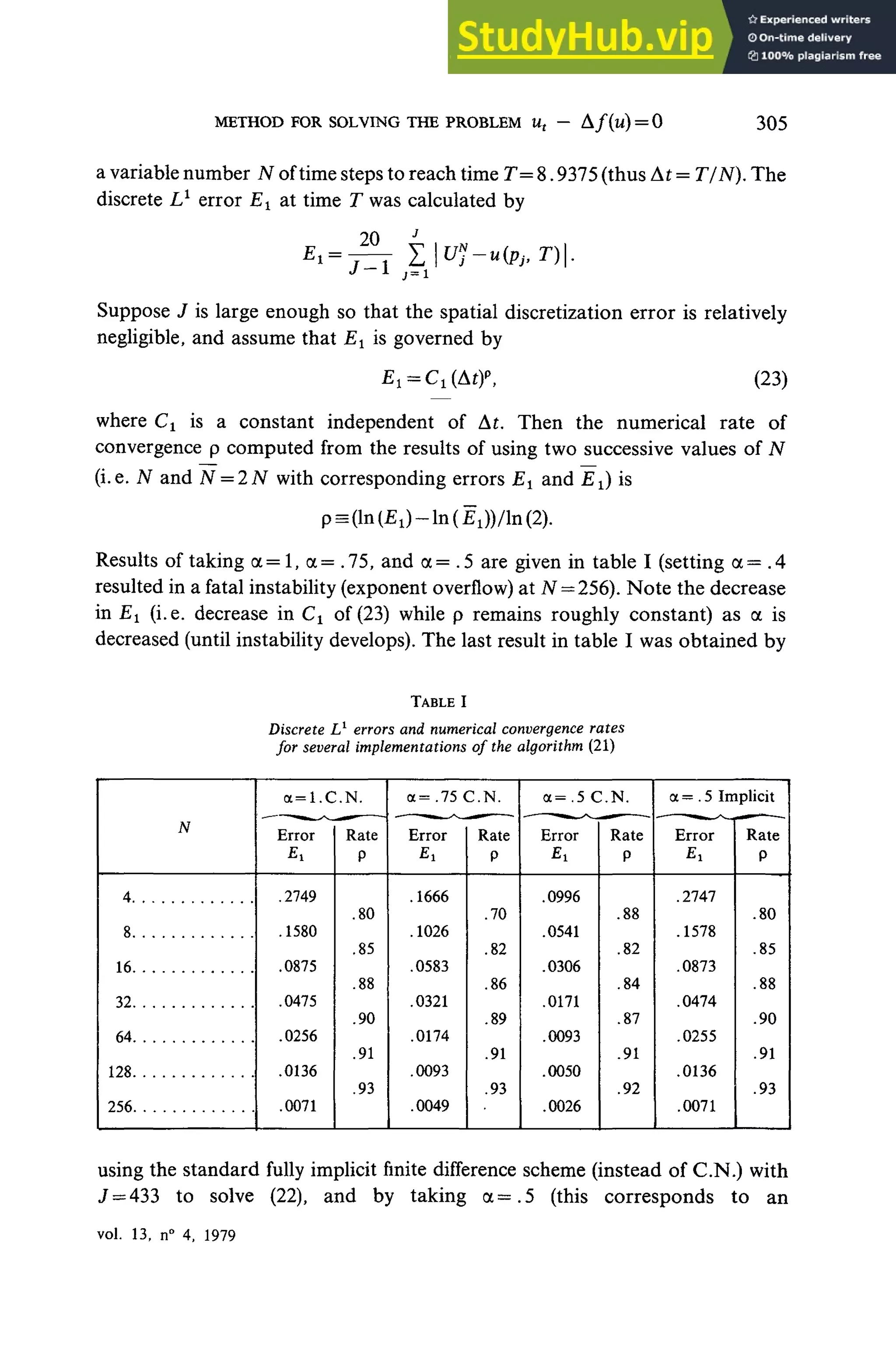
11. 306 A. E. BERGER, H. BRÉZIS, J. C. W. ROGERS
implementation of a form of the Laplace modified forward Galerkin method
— c.f. p. 154of [16]).Notice the almost exact correspondence between the results
for (a = .5, implicit) and those for (a— 1, C.N.). This correspondence also occurs
between (a = .375, implicit) and (a= .75, C.N.), and between (oc = .25, implicit)
and (a = .5, C.N.) (J =433 throughout). Taking a = .2 with the implicit method
(J = 433) yields instability at A
f= 256. The plausibility of this correspondence
may be seen by writing out the algorithm (21) using the appropriate matrix K
for the scheme being used for (22), and here taking Un
to be the vector of values
{ L/"; pjGT}, etc. and assuming zero Dirichlet data
ƒ(£/") -f{U»)
For C.N., 9= 1/2, while for implicit, 0= 1 in this expression.
Alittle algebra shows that taking (C.N., a = a )is identical to taking (implicit,
a = a /2). Some more algebra shows that including the effect ofnonzero Dirichiet
data yields a formally O(At) différence between (C.N,, a = a) and (implicit,
<
x = a/2). Since the boundary data for this example is zero until t is near
r=8.9375, the numerical agreement is very pronounced, despite the fact that
the observed numerical error of the algorithm itself is behaving almost like
O (At). As an indication of the effect of the size of J on the error; with N = 256,
a= .5, and using C.N. for (22), the values of £, corresponding to several values
of J were;
f^.0177
109
.0044
217
.0042
433
.0026
For comparison, we also implemented the 3 Ievel (centered) Laplace modified
Galerkin équation {see p. 155 of [16]) for (20), in the foliowing form [here
Dl Uj^iUj-i-2 Uj+ *7j+1)/Ax2
and Ax is the (uniform) mesh length];
+ 2AD2
x(f(U'})) forysuchthatO<p;<20. (24)
The exact solution was used to provide the values U) at t= At. Results are given
in table II (again J = 433 and T=8.9375). The condition on the parameter p
given in [16] (for "smooth" problems) is p> |x/4 (here (3= .25 satisfies this while
R.A.I.R.O. Analyse numérique/Numerical Analysis

12. METHOD FOR SOLVING THE PROBLEM Ut - Af(u) = 307
P=.2 does not). Taking p = .15 yields instabiiity (exponent overflow) at
N =256. For N = 256 and P= .25 one has;
7 =55
Ei =.0163
109
.0028
217
.0023
433
.0005
Even for this (nonsmooth) problem, the 3 level scheme produces a higher
numerical rate of convergence.
TABLE II
Discrete L1
errors and numerical convergence rates
for several implementations of the Laplace modified centered équation (24)
N
4
8
16
32
64
128
256
P=-
Error
Ei
1.572
.4853
.1637
.0609
.0224
.0079
.0021
1
_
_
^ —
Rate
P
1.7
1.6
1.4
1.4
1.5
1.9
Error
Ei
.7560
.2160
.0854
.0349
.0139
.0048
.0009
5
Rate
P
1.8
1.3
1.3
1
.
3
1.5
2.4
p=.25
Error
.3175
.1179
.0485
.0212
.0084
.0024
.0005
Rate
P
1.4
1.3
1.2
1.3
1.8
2.3
Error
Ex
.2537
.1043
.0475
.0193
.0072
.0018
.0005
l
Rate
P
1.3
1.1
1.3
1.4
2.0
2.0
The second problem to be considered is a two phase Stefan problem whose
solution (in terms of température) is depicted in ïigtwe 2 (the exact solution is
given in both [7] and [20] —note that in this panicular example x= ki/Ci and
z= z"=ri = 0).In order to suppress the effect of thejump discontinuity from 0 toX
in enthalpy at the interface, errors discussed hère for the Stefan problem will be
errors in température values. The température v corresponding to an enthalpy
value u is easily obtained by inverting (6).
For the one phase Stefan problem, the alternating phase truncation (APT)
method ([7, 20]) reduces to (21) with a = i. In [20], for the "analytical" APT
method for a one dimensional one phase Stefan problem, it was shown that the
vol. 13. n° 4, 1979

13. 308 A. E. BERGER, H. BRÉZIS, J. C. W. ROGERS
Figure 2. —Exact solution (température) of a two phase Stefan problem (solid Unes) and numerical
solution values (points) at t = 0, t = 773 (triangles), t = 2 773 (open circles), and t = T (solid circles)
where T= 200,000. The approximate solution values were obtained using the algorithm (21) with
a = kjclt and using the standard Crank-Nicolson finite différence method with 41 grid points and
At= 772,595 tosolVe (22).
error in the température value and in the interface location could be bounded by
Un(l + T/At))1/2
, (25)
where T is the time at which one is bounding the error, and C is a constant
independent of At (but depending on T and the data of the problem). Let N
dénote the integer T/At, so then f*=N At=T. We have tested to see if the
temporal error behavior for (21) applied to the two phase Stefan problem is
consistent with (25) by fixing T, taking J "large", and calculating numerical
values for C for several values of Àt. Let v(x, t*) dénote the exact température
solution at time t? = Tt and let {Vf} dénote the approximate température
solution values at the grid points {pj} at time tN
obtained via (21) [i.e. V1
-is
defined to be the température corresponding (by (6)) to Uf]. The discrete Ll
error ex is defined to be
e =.
20 i.
and the numerical value of C corresponding to N (i.e. to At = T/N) is
(26)
(27)
R.A.I.R.O. Analyse numérique/Numerical Analysis

14. METHOD FOR SOLVÏNG THE PROBLEM Ut — A ƒ (tt) = 0 309
Results of applying the algorithm (21) to the two phase Stefan problem are
given in tables III and IV In all the tables for the Stefan problem
T= (2/3) 200,000 For table III, the standard Crank-Nicolson (C N ) method
TABLE III
Discrete L1
errors e1 and values of the constant C of (21)for several implementations of the algorithm
(21) and an implementatwn of the APT method for the two phase Stefan problem
A
216
432
864
1728
3 456
a = l 3n
ei j
9 10
6 81
4 75
3 46
2 43
C N
C
16
16
15
14
14
a = n C
10 16
6 63
4 40
3 06
2 22
N
C
18
15
14
13
13
a= 96 n
«i
84 6
89 8
88 9
88 2
82 1
C N
C
1 5
2 1
2 8
3 7
4 6
APTC
12 26
8 69
5 87
4 20
2 99
N
C
21
20
18
18
17
TABLE IV
Discrete L1
errors et and values of the constant C of {21)for several implementations of the algorithm
(21) for the two phase Stefan problem The Standard implicit method with J = 161 was used to
solve (22)
N
ot= 48 n
216
432
864
1728
3 456
1125
8 05
5 82
4 19
3 00
20
19
18
17
17
12
83
75
46
43
16
16
15
14
14
1025
6 76
4 39
3 02
2 22
18
16
14
13
13
92 0
92 3
89 7
87 4
82 1
1 6
2 1
2 8
3 6
4 6
with J = 161wasused to solve (22),results are given for a = 1 3,1,and 95 u, and
for companson, results for the APT method (C N ,J = 161) are given m the last
column The error behavior appears consistent with (25) The error decreases as
o
cdecreases until the abrupt détérioration below o
c = u Results when usmg the
Standard implicit method for (22) with J = 16i are given m table IV The
correspondence between (CN,a) and (implicit, a/2) is again observed [this is
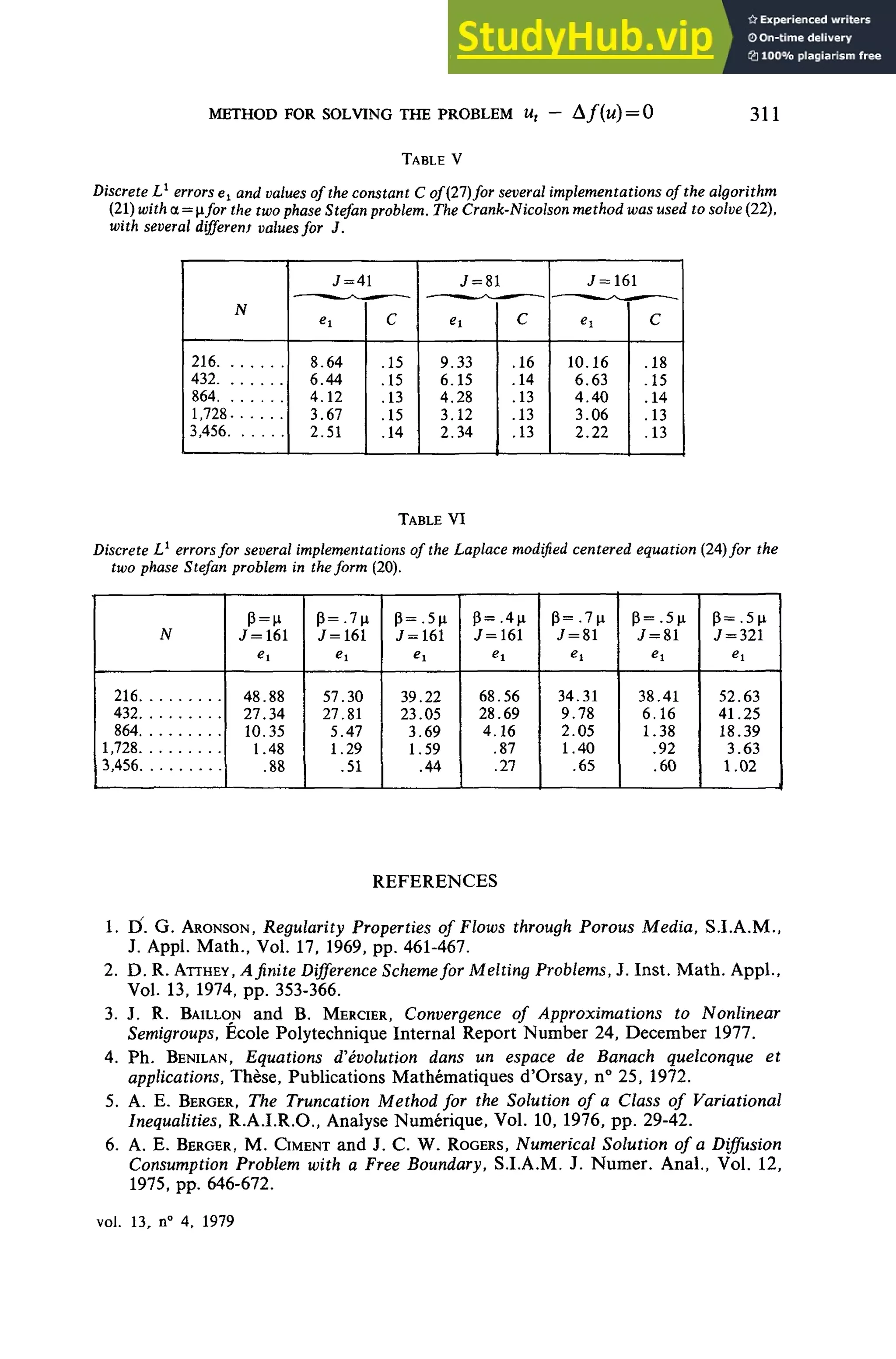
not surpnsmg since O (At) is "small" relative to (25)] The data m table V
mdicates that for the values of JV being considered, the spatial discretization
error is relatively neghgible even for J = 41 We note that the method for the
Stefan problem discussed m [2] and [21] corresponds to using a purely explicit
method to solve (20) The 3 level Laplace modified Galerkin method (24) when
vol 13 n° 4 1979

15. 310 A. E. BERGER, H. BRÉZIS, J. C, W. ROGERS
applied to the Stefan problem in the form (20)produced very erratic behavior
with respect to variations in both P and J (typical behavior is presented in
table VI). Fatal instability occurs with J=161, p= .3(a,N= 3,456.
As an illustration of the simplicity of using (21)in several space dimensions,
numerical results for a twodimensional Stefan problem aregiven infigure 3. The
LLLLLLLLLLLLLLLLLLLLL
LLLLLLLLLLLLLLLLLLILL
LLLLLLLLLLLLLLLLLLLLL
LLLLLLLLLLLLLLLLLLLLL
LLLLLLLLLLLLLLLLLLLLt
LLLLLLLLLLLLLLLLLLLLL
LLLLLLLLLLLLLLLLLLLLL
LLLLLL-LLLLLLLLLLLLLL
LLLLLLLLLLLLLLLLLLLLL
LLLLLLLLLLLLLLLLLLLLL
LLLLLLLLLLLLLL.LLLLLLL
LLLLLLLLLLLLLLLLLLLLL
LLLLLLLLLLLLLLLLLLLLL
LLLLLLLLLLLLLLLLLLLLL
LLLLLLLLLLLLLLLLLLLLL
LLLLLLLLLLLLLLLLLLLLL
LLLLLi-LLi-LLLLlLLLLlLJÊ
LLLLLLLLLLLLLLLLLLL/S
LLLLLLLL LLLLLLL LL_LJSS
LLLLLLLLLLLLLLLLLL£SS
LLLLLLLLLLLLLLLLLl/SSS
L L L L L L L L L L ' - U L L L L L L L L L
LLLLLLLLLLLLLLLLLLuLL
LLLLLLLLLLLLLLLLLLLLL
LLLLLLLLLLLLLLLLLLLLL
LLLLLLLLLL LLLLLLLLLLc
LLLLLLLLLLLLLLLLLLLLL
L L L L L ' - L L - L L L L L L L L ^ L L L
LLLLLLLLLLLLLLLLLLLLL
LLLLLLLLLLLLLLLLLLLLL
LLLLLLLLLLLLLLLLLLLLÉ
LLLLLLLLLLLLLLLLLtL/S
LLLLLLLL LLLLLL LLLLL/S
LLLLLL LLLLLLLLLLLL h S
/
LLLLLLLLLLLLLLLLL/S3S
LL LLLLLL L L L L L L L L / 3 SCi
LLLLLLLLL L L /
LLLLLLLLLLLLLLL/
LLLLLLLLLLLLLL/SSbSSS
/
LLLLLL LLLLLLI-L L L L L L L L
L L L L ' - L L L L L L L L L L L L L L I L
LLLLLLLLLLLL LLLLLL LL f
LLLLLLLL LLLL LL LL LL Lij
LLLLLLLLLLLL-LLLLLL
LuLLLLLLL'.LL LLLLLL J
LLLLLLLL LLLL-.LLLLL/
LLLLLL'.L LLLLLL LLL/SSÎ,
LLLLLLLLLLLLLLLL1/
LLLLLLLL LLLLLLLL/S S--s
L L L L L L ' - L L L L L L L L ' J SS31
LLLLLLLLLLLLLLL/ SbSSJ
LLLLLLLLLLLLL
LLLLuLLLLLLI
LLLLLLLLLLLI
LLLLLLLLLLLI
LLLLLLLLLLLI
t = T/3
LLLLLLLLLLL
L L L L L L L L L L L L L L L L L / S S S
LLLLLLLLLLLLLLLL/5SSJ
LLLLLLLLLLLLLLLU
LLLLLLLLLLLLLLL/ S3S*ÎS
LLLLLLLLLLLLLLt/ S^SSS
LL LL LL LL LL LL LL/ 5S - S
S S
LLLLLLLLLLLLL/SSSSSSS
L L L L L L L L L L L L L / S^S5r
S5
LLLLLLLLLlLL/"SSS
LLLLLLLLLLLL
LLLLLLLLLLy
LLLLLL Lt LL/S3^S"SSSS 5
LL L L L L LL L/IC "S <ÎS SS SSS
LLLLLLLLL/ESSSS-^'ÎSSS
LLtLLLLL/S^SSS^'SSSSS
LLLLLLLL
LLLLLLL S SSS3 S3 SS5
LLLLL LLLLLLLL LLLLI/S^S
LLLLLLLLLLLLLLLLL
LLLLLLLLLLLLLLLL/
LLLLLLLLLLLLLLL i
LLLLLLLLLLLLLLL/
LLLLLLLLLLLLLL,
LLLLLLLLLLLLLL/
LLLLLLLLLLLLL/
LLLLLLULLLL
LLLLLLLLLLLL^
LLLLLLLLLLL
LLLLLLLLLLL/
LLLLLLLLLLy
LLLLLLLLLL/
LLLLLLLLL>
LLLLLLLL
LLLLLLLL
LLLLLLL
LLLLLLL
LLLLLL
LLLLLL
t=T
Figure 3. - Numerical solution of a two phase Stefan problem on the région O^x, y^20 using the
algorithm (21)with a = /c,7c,-. In each frame, an L(S)wasprinted at points where the approximate
solution value was ^ A.(^ 0). A blank wasprinted forvalues between 0 and X.Thesolid line isthe
exact interface location. Thestandard ADI method [19]with Ax= Ay = 1, wasused to solve(22).
For the first four frames the value of At used was 775,184 (7=200,000). For the frame onthe
lower rigbt the value of At was 77648.
classical ADImethod [19] wasused tosolve (22).Theexact solution at (x, y, t) is
given by u(p= x cos(30°) - y. sin(30°), t)where u is thesolution in [7],[20](p is
the projection of(x, y) on the line 30°below the positive x-axis, note also that
i=ki/ci and z= z—r1 =0).
R.A.Ï.R.O. Analyse mimérique/Numerical Analysis

16. METHOD FOR SOLVING THE PROBLEM Ut - Af(u) = 311
TABLE V
Discrete Ll
errors ex andvalues of the constant C of(21)for several implementations of the algorithm
(21) with a - ifor the twophase Stefan problem. TheCrank-Nicolson method was used to solve (22),
with several different values for J.
N
216
432
864
1,728
3,456.
J = 41
ei
8.64
6.44
4.12
3.67
2.51
C
.15
.15
.13
.15
.14
J-81
ei
9.33
6.15
4.28
3.12
2.34
L
c
.16
.14
.13
.13
.13
J = 16
ei
10.16
6.63
4.40
3.06
2.22
1
C
.18
.15
.14
.13
.13
TABLE VI
Discrete L1
errorsfor several implementations of the Laplace modified centered équation (24) for the
two phase Stefan problem in the farm (20).
JV
216
432
864
1,728
3,456
ei
48.88
27.34
10.35
1.48
.88
J=161
ei
57.30
27.81
5.47
1.29
.51
ei
39.22
23.05
3.69
1.59
.44
ei
68.56
28.69
4.16
.87
.27
J =81
ei
34.31
9.78
2.05
1.40
.65
38.41
6.16
1.38
.92
.60
ei
52.63
41.25
18.39
3.63
1.02
REFERENCES
1. D. G. ARONSON, Regularity Properties of Flows through Porous Media, S.I.A.M.,
J. Appl. Math., Vol.17, 1969, pp.461-467.
2. D.R.ATTHEY, Afinite Différence Schemefor Melting Problems, J. Inst. Math. Appl.,
Vol. 13,1974, pp.353-366.
3. J. R. BÂILLON and B. MERCIER, Convergence of Approximations to Nonlinear
Semigroups, École Polytechnique Internai Report Number 24, December 1977.
4. Ph. BENILAN, Equations dévolution dans un espace de Banach quelconque et
applications, Thèse, Publications Mathématiques d'Orsay, n° 25, 1972.
5. A. E. BERGER, The Truncation Method for the Solution of a Class of Variational
Inequalities, R.A.LR.O., Analyse Numérique, Vol. 10, 1976, pp. 29-42.
6. A. E. BERGER, M. CIMENT and J. C. W. ROGERS, Numerical Solution of a Diffusion
Consumption Problem with a Free Boundary, S.LA.M. J. Numer. Anal., Vol. 12,
1975, pp.646-672.
vol. 13,n° 4, 1979

17. 312 A. E. BERGER, H. BRÉZIS, J. C. W. ROGERS
7. A. E. BERGER, M. CIMENT and J. C. W. ROGERS, Numerical Solution ofa Stefan Problem
by a Technique of Alternating Phase Truncation, Séminaires IRIA, Analyse et
contrôle des systèmes, Rocquencourt, Institut de Recherche d'Informatique et
d'automatique, 1976, pp. 21-34.
8. A. E. BERGER and R. S. FALK, An ErrorEstimatefor the Truncation Methodfor the
Solution ofParabolic Obstacle Variational Inequalities, Math. Comp., Vol. 31,1977,
pp. 619-628.
9. H. BREZIS, On Some Degenerate Nonlinear Parabolia Equations, Nonlinear
Functional Analysis, F. BROWDER, Ed., Proc. Symp. in pure math., Vol. 18,
A.M.S., 1970, pp. 28-38.
10. H. BREZIS and A. PAZY, Convergence andApproximation of Semigroups of Nonlinear
Operators in Banach Spaces, J. Func. Anal., Vol. 9, 1972, pp. 63-74.
IL H. BREZIS and W. A. STRAUSS, Semi-Linear Second OrderElliptic Equations in L1
,
J. Math. Soc. Japan, Vol. 25, 1973, pp. 565-590.
12. M. G. CRANDALL, An Introduction to Evolution Governed by Accretive Operators,
Dynamical Systems vol. 1, Proc. of the Int. Symp. on Dyn. Sys. at Brown U.
August 12-16, 1974, L. CESARI, J. K. HALE and J. P. LASALLE, Eds, New York,
Academie Press, 1976, pp. 131-165.
13. M. G. CRANDALL, Semigroups of Nonlinear Transformationsin Banach Spaces,
Contributions to nonlinearFunctionalAnalysis, E. ZARANTONELLO, Ed., New York,
Academie Press, 1971, pp. 157-179.
14. M. G. CRANDALL and T. M. LIGGETT, Générationof Semi-groups of Nonlinear
Transformations on General Banach Spaces, Amer. J. Math., Vol. 93, 1971,
pp. 265-298.
15. A. DAMLAMIAN, Some Results on theMulti-phase StefanProblem, Comm. on P.D.E.,
Vol. 2, 1977, pp. 1017-1044.
16. J. DOUGLAS Jr. and T. DUPONT, Alternating-Direction Galerkin Methods on
Rectangles, Numerical Solution of Partial DifferentialEquaîions-ll, SYNSPADE
1970, B. HUBBARD, Ed., New York, Academie press, 1971, pp. 133-214.
17. B. H. GILDING and L. A. PELETIER, On a Classof Similarity Solutionsof the Porous
Media Equation, J. Math. Anal. Appl., Vol. 55, 1976, pp. 351-364.
18. B. H. GILDING and L. A. PELETIER, On a Classof SimilaritySolutionsof the Porous
Media Equation II, J. Math. Anal. Appl., Vol. 57, 1977, pp. 522-538.
19. D. W. PEACEMAN and H. H. RACHFORD Jr., The Numerical SolutionofParabolic and
Elliptic Differential Equations, J. Soc. Indust; Appl. Math., Vol. 3, 1955, pp. 28-41.
20. J. C. W. ROGERS, A. E. BERGER and M. CIMENT, The AlternatingPhase Truncation
Method for Numerical Solution of a Stefan Problem, to appear in S.LA.M.
J. Num. Anal.
21. M. ROSÉ, A Methodfor CalculatingSolutions of ParabolieEquationswith a Free
Boundary, Math. Comp., Vol. 14, 1960, pp. 249-256.
R.A.I.R.O. Analyse numérique/Numerical Analysis