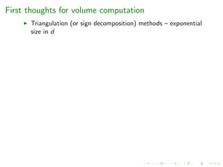
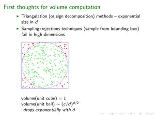
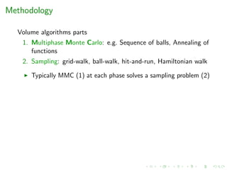
Download as PDF, PPTX


![Birkhoff polytopes
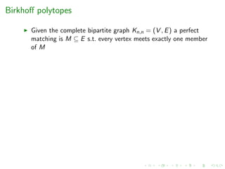
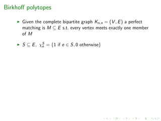
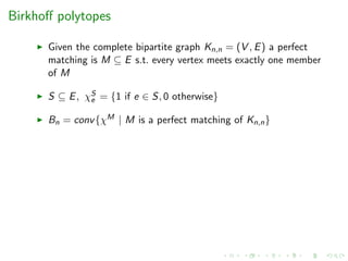
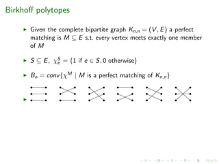
Given the complete bipartite graph Kn,n = (V , E) a perfect
matching is M ⊆ E s.t. every vertex meets exactly one member
of M
S ⊆ E, χS
e = {1 if e ∈ S, 0 otherwise}
Bn = conv{χM | M is a perfect matching of Kn,n}
# faces of B3: 6, 15, 18, 9; vol(B3) = 9/8
there exist formulas for the volume [deLoera et al ’07] but
values only known for n ≤ 10 after 1yr of parallel computing
[Beck et al ’03]](https://image.slidesharecdn.com/uoa19-200124130040/85/A-new-practical-algorithm-for-volume-estimation-using-annealing-of-convex-bodies-9-320.jpg)
![Volumes and counting
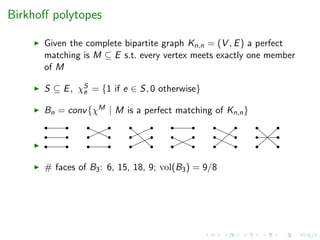
Given n elements & partial order; order poly-
tope PO ⊆ [0, 1]n coordinates of points satisfies the partial order
c
a
b a, b, c
partial order: a < b
3 linear extensions: abc, acb, cab](https://image.slidesharecdn.com/uoa19-200124130040/85/A-new-practical-algorithm-for-volume-estimation-using-annealing-of-convex-bodies-10-320.jpg)
![Volumes and counting
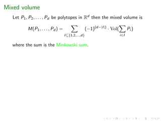
Given n elements & partial order; order poly-
tope PO ⊆ [0, 1]n coordinates of points satisfies the partial order
c
a
b a, b, c
partial order: a < b
3 linear extensions: abc, acb, cab
# linear extensions = volume of order polytope · n!
[Stanley’86]](https://image.slidesharecdn.com/uoa19-200124130040/85/A-new-practical-algorithm-for-volume-estimation-using-annealing-of-convex-bodies-11-320.jpg)
![Volumes and counting
Given n elements & partial order; order poly-
tope PO ⊆ [0, 1]n coordinates of points satisfies the partial order
c
a
b a, b, c
partial order: a < b
3 linear extensions: abc, acb, cab
# linear extensions = volume of order polytope · n!
[Stanley’86]
Counting linear extensions is #P-hard [Brightwell’91]](https://image.slidesharecdn.com/uoa19-200124130040/85/A-new-practical-algorithm-for-volume-estimation-using-annealing-of-convex-bodies-12-320.jpg)
![Volumes and algebraic geometry
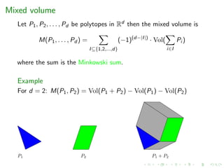
Toric geometry
If P is an integral d-dimensional polytope, then d! times the volume
of P is the degree of the toric variety associated to P.
BKK bound (Bernshtein, Khovanskii, Kushnirenko)
Let f1, . . . , fn be polynomials in C[x1, . . . , xn]. Let N(fj ) denote the
Newton polytope of fj , i.e. the convex hull of it’s exponent vectors.
If f1, . . . , fn are generic, then the number of solutions of the
polynomial system of equations
f1 = 0, . . . , fn = 0
with no xi = 0 is equal to the normalized mixed volume
n!M(N(f1), . . . , N(fn))](https://image.slidesharecdn.com/uoa19-200124130040/85/A-new-practical-algorithm-for-volume-estimation-using-annealing-of-convex-bodies-15-320.jpg)
![Applications
Volume of zonotopes is used to test methods for order
reduction which is important in several areas: autonomous
driving, human-robot collaboration and smart grids [Althoff et
al.]
Volumes of intersections of polytopes are used in bio-geography
to compute biodiversity and related measures e.g. [Barnagaud,
Kissling, Tsirogiannis, Fisikopoulos, Villeger, Sekercioglu’17]](https://image.slidesharecdn.com/uoa19-200124130040/85/A-new-practical-algorithm-for-volume-estimation-using-annealing-of-convex-bodies-16-320.jpg)
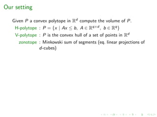
![Our setting
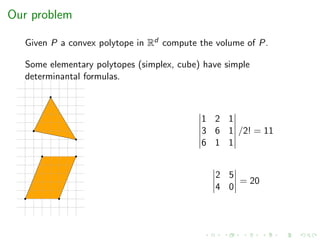
Given P a convex polytope in Rd compute the volume of P.
H-polytope : P = {x | Ax ≤ b, A ∈ Rq×d , b ∈ Rq}
V-polytope : P is the convex hull of a set of points in Rd
zonotope : Minkowski sum of segments (eq. linear projections of
d-cubes)
Complexity
#P-hard for both representations [DyerFrieze’88]](https://image.slidesharecdn.com/uoa19-200124130040/85/A-new-practical-algorithm-for-volume-estimation-using-annealing-of-convex-bodies-20-320.jpg)
![Our setting
Given P a convex polytope in Rd compute the volume of P.
H-polytope : P = {x | Ax ≤ b, A ∈ Rq×d , b ∈ Rq}
V-polytope : P is the convex hull of a set of points in Rd
zonotope : Minkowski sum of segments (eq. linear projections of
d-cubes)
Complexity
#P-hard for both representations [DyerFrieze’88]
open if both representations available](https://image.slidesharecdn.com/uoa19-200124130040/85/A-new-practical-algorithm-for-volume-estimation-using-annealing-of-convex-bodies-21-320.jpg)
![Our setting
Given P a convex polytope in Rd compute the volume of P.
H-polytope : P = {x | Ax ≤ b, A ∈ Rq×d , b ∈ Rq}
V-polytope : P is the convex hull of a set of points in Rd
zonotope : Minkowski sum of segments (eq. linear projections of
d-cubes)
Complexity
#P-hard for both representations [DyerFrieze’88]
open if both representations available
no deterministic poly-time algorithm can compute the volume
with less than exponential relative error (oracle
model) [Elekes’86]](https://image.slidesharecdn.com/uoa19-200124130040/85/A-new-practical-algorithm-for-volume-estimation-using-annealing-of-convex-bodies-22-320.jpg)
![State-of-the-art
Authors-Year Complexity Algorithm
(oracle steps)
[Dyer, Frieze, Kannan’91] O∗(d23) Sequence of balls + grid walk
[Kannan, Lovasz, Simonovits’97] O∗(d5) Sequence of balls + ball walk + isotropy
[Lovasz, Vempala’03] O∗(d4) Annealing + hit-and-run
[Cousins, Vempala’15] O∗(d3) Gaussian cooling (* well-rounded)
[Lee, Vempala’18] O∗(Fd
2
3 ) Hamiltonian walk (** H-polytopes)](https://image.slidesharecdn.com/uoa19-200124130040/85/A-new-practical-algorithm-for-volume-estimation-using-annealing-of-convex-bodies-23-320.jpg)
![State-of-the-art
Authors-Year Complexity Algorithm
(oracle steps)
[Dyer, Frieze, Kannan’91] O∗(d23) Sequence of balls + grid walk
[Kannan, Lovasz, Simonovits’97] O∗(d5) Sequence of balls + ball walk + isotropy
[Lovasz, Vempala’03] O∗(d4) Annealing + hit-and-run
[Cousins, Vempala’15] O∗(d3) Gaussian cooling (* well-rounded)
[Lee, Vempala’18] O∗(Fd
2
3 ) Hamiltonian walk (** H-polytopes)
Software:
[Emiris, F’14] Sequence of balls + coordinate hit-and-run
[Cousins, Vempala’16] Gaussian cooling + hit-and-run](https://image.slidesharecdn.com/uoa19-200124130040/85/A-new-practical-algorithm-for-volume-estimation-using-annealing-of-convex-bodies-24-320.jpg)
![State-of-the-art
Authors-Year Complexity Algorithm
(oracle steps)
[Dyer, Frieze, Kannan’91] O∗(d23) Sequence of balls + grid walk
[Kannan, Lovasz, Simonovits’97] O∗(d5) Sequence of balls + ball walk + isotropy
[Lovasz, Vempala’03] O∗(d4) Annealing + hit-and-run
[Cousins, Vempala’15] O∗(d3) Gaussian cooling (* well-rounded)
[Lee, Vempala’18] O∗(Fd
2
3 ) Hamiltonian walk (** H-polytopes)
Software:
[Emiris, F’14] Sequence of balls + coordinate hit-and-run
[Cousins, Vempala’16] Gaussian cooling + hit-and-run
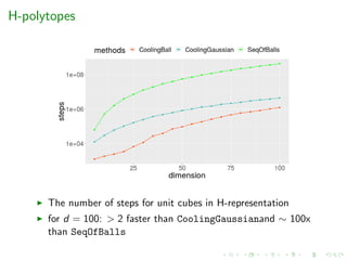
Limitation: Efficient only for H-polytopes (scale up-to few hundred
dims in hrs), for V-polytopes or zonotopes:
oracles are expensive (solution of an LP)
[Cousins, Vempala’16] needs a bound on the number of facets](https://image.slidesharecdn.com/uoa19-200124130040/85/A-new-practical-algorithm-for-volume-estimation-using-annealing-of-convex-bodies-25-320.jpg)
![State-of-the-art
Authors-Year Complexity Algorithm
(oracle steps)
[Dyer, Frieze, Kannan’91] O∗(d23) Sequence of balls + grid walk
[Kannan, Lovasz, Simonovits’97] O∗(d5) Sequence of balls + ball walk + isotropy
[Lovasz, Vempala’03] O∗(d4) Annealing + hit-and-run
[Cousins, Vempala’15] O∗(d3) Gaussian cooling (* well-rounded)
[Lee, Vempala’18] O∗(Fd
2
3 ) Hamiltonian walk (** H-polytopes)
Software:
[Emiris, F’14] Sequence of balls + coordinate hit-and-run
[Cousins, Vempala’16] Gaussian cooling + hit-and-run
Limitation: Efficient only for H-polytopes (scale up-to few hundred
dims in hrs), for V-polytopes or zonotopes:
oracles are expensive (solution of an LP)
[Cousins, Vempala’16] needs a bound on the number of facets
Goal: Efficient algorithm for V-polytopes and zonotopes](https://image.slidesharecdn.com/uoa19-200124130040/85/A-new-practical-algorithm-for-volume-estimation-using-annealing-of-convex-bodies-26-320.jpg)
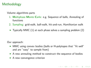
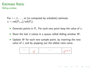
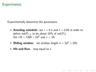
![Annealing Schedule
How we compute the sequence of bodies
Inputs: Polytope P, error , cooling parameters r, δ > 0 and a
significance level (s.l.) α > 0 s.t. 0 < r + δ < 1.
Output: A sequence of convex bodies C1 ⊇ · · · ⊇ Cm s.t.
vol(Pi+1)/vol(Pi ) ∈ [r, r + δ] with high probability
where Pi = Ci ∩ P, i = 1, . . . , m and P0 = P.](https://image.slidesharecdn.com/uoa19-200124130040/85/A-new-practical-algorithm-for-volume-estimation-using-annealing-of-convex-bodies-30-320.jpg)
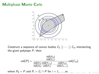
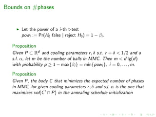
![t-test
for the ratio of volumes of convex bodies
Given convex bodies Pi ⊇ Pi+1, s.l. α, and cooling parameters
r, δ > 0, 0 < r + δ < 1, we define two t-tests:
testL(Pi , Pi+1, r, δ, α, ν, N): testR(Pi , Pi+1, r, α, ν, N):
H0 : vol(Pi+1)/vol(Pi ) ≤ r + δ H0 : vol(Pi+1)/vol(Pi ) ≤ r
H1 : vol(Pi+1)/vol(Pi ) ≥ r + δ H1 : vol(Pi+1)/vol(Pi ) ≥ r
Successful if we fail to reject H0 Successful if we reject H0
testL and testR are used by annealing schedule to restrict
each ratio ri = vol(Pi+1)/vol(Pi ) in the interval [r, r + δ].](https://image.slidesharecdn.com/uoa19-200124130040/85/A-new-practical-algorithm-for-volume-estimation-using-annealing-of-convex-bodies-32-320.jpg)
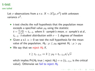
![t-test
Compute testL, testR for Pi ⊇ Pi+1
1. sample νN points from Pi and split the sample into ν sublists
of length N.
2. The ν mean values are experimental values that follow
N(ri , (ri (1 − ri ))/N).
3. Use those values to perform two t-tests with null hypotheses:
testL H0 : ri ≤ r + δ testR H0 : ri ≤ r
Assuminga
the following holds,
r + δ + tν−1,α
s√
ν
≥ ˆµ ≥ r + tν−1,α
s√
ν
then ri is restricted to [r, r + δ] with high probability.
a
for the mean ˆµ of the ν mean values](https://image.slidesharecdn.com/uoa19-200124130040/85/A-new-practical-algorithm-for-volume-estimation-using-annealing-of-convex-bodies-33-320.jpg)
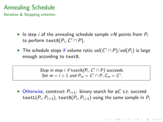
![Initialization of Annealing Schedule
Given: polytope P, convex body C s.t. C ∩ P = ∅, an interval
[qmin, qmax] and parameters r, δ, α, ν, N.
binary search for q ∈ [qmin, qmax] s.t. both testL(qC, qC ∩ P)
and testR(qC, qC ∩ P) are successful.
sample from qC, rejection to P
we call the successful qC, C](https://image.slidesharecdn.com/uoa19-200124130040/85/A-new-practical-algorithm-for-volume-estimation-using-annealing-of-convex-bodies-34-320.jpg)
![1st iteration of the initialization step
[qmin, qmax] = [0.14, 0.38], q = qmin+qmax
2 = 0.26
r = 0.8, δ = 0.05, α = 0.1, ν = 10, νN = 1200 ⇒ N = 120
ˆµ = r (1)+r (2)···+r (10)
ν = 684
1200 = 0.57, s = 0.06
testL→ H0 : volqC∩P
vol(qC)
≤ r + δ ⇒ succeed (H0 not rejected).
testR→ H0 : volqC∩P
vol(qC)
≤ r ⇒ failed (H0 not rejected).
qC of 1st iteration is too big (the ratio is too small).](https://image.slidesharecdn.com/uoa19-200124130040/85/A-new-practical-algorithm-for-volume-estimation-using-annealing-of-convex-bodies-35-320.jpg)
![2nd iteration of the initialization step
[qmin, qmax] = [0.14, 0.26], q = qmin+qmax
2 = 0.20
r = 0.8, δ = 0.05, α = 0.1, ν = 10, νN = 1200 ⇒ N = 120
ˆµ = r (1)+r (2)···+r (10)
ν = 914
1200 = 0.76, s = 0.04
testL→ H0 : volqC∩P
vol(qC)
≤ r + δ ⇒ succeed (H0 not rejected).
testR→ H0 : volqC∩P
vol(qC)
≤ r ⇒ failed (H0 not rejected).
qC of 2nd iteration is too big (the ratio is too small).](https://image.slidesharecdn.com/uoa19-200124130040/85/A-new-practical-algorithm-for-volume-estimation-using-annealing-of-convex-bodies-36-320.jpg)
![3rd iteration of the initialization step
[qmin, qmax] = [0.14, 0.20], q = qmin+qmax
2 = 0.17
r = 0.8, δ = 0.05, α = 0.1, ν = 10, νN = 1200 ⇒ N = 120
ˆµ = r (1)+r (2)···+r (10)
ν = 1076
1200 = 0.90, s = 0.02
testL→ H0 : volqC∩P
vol(qC)
≤ r + δ ⇒ failed (H0 rejected).
testR→ H0 : volqC∩P
vol(qC)
≤ r ⇒ succeed (H0 rejected).
qC of 3rd iteration is too small (the ratio is too big).](https://image.slidesharecdn.com/uoa19-200124130040/85/A-new-practical-algorithm-for-volume-estimation-using-annealing-of-convex-bodies-37-320.jpg)
![4th iteration of the initialization step
[qmin, qmax] = [0.17, 0.20], q = qmin+qmax
2 = 0.185
r = 0.8, δ = 0.05, α = 0.1, ν = 10, νN = 1200 ⇒ N = 120
ˆµ = r (1)+r (2)···+r (10)
ν = 993
1200 = 0.83, s = 0.04
testL→ H0 : volqC∩P
vol(qC)
≤ r + δ ⇒ succeed (H0 not rejected).
testR→ H0 : volqC∩P
vol(qC)
≤ r ⇒ succeed (H0 rejected).
Set C = qC.](https://image.slidesharecdn.com/uoa19-200124130040/85/A-new-practical-algorithm-for-volume-estimation-using-annealing-of-convex-bodies-38-320.jpg)
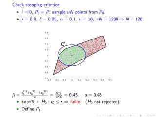
![Define next convex body in MMC
i = 0, P0 = P, binary search for q ∈ [0.185, 0.38]
r = 0.8, δ = 0.05, α = 0.1, ν = 10, νN = 1200 ⇒ N = 120
q = 0.36, ˆµ =
r
(1)
0 +r
(2)
0 ···+r
(10)
0
ν = 998
1200 = 0.83, s = 0.07
testL→ H0 : r0 ≤ r + δ ⇒ succeed (H0 not rejected).
testR→ H0 : r0 ≤ r ⇒ succeed (H0 rejected).
Set C1 = qC.](https://image.slidesharecdn.com/uoa19-200124130040/85/A-new-practical-algorithm-for-volume-estimation-using-annealing-of-convex-bodies-41-320.jpg)
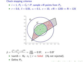
![Define next convex body in MMC
i = 1, P1 = C1 ∩ P, binary search for q ∈ [0.185, 0.36]
r = 0.8, δ = 0.05, α = 0.1, ν = 10, νN = 1200 ⇒ N = 120
q = 0.28, ˆµ =
r
(1)
1 +r
(2)
1 ···+r
(10)
1
ν = 998
1200 = 0.82, s = 0.06
testL→ H0 : r1 ≤ r + δ ⇒ succeed (H0 not rejected).
testR→ H0 : r1 ≤ r ⇒ succeed (H0 rejected).
Set C2 = qC.](https://image.slidesharecdn.com/uoa19-200124130040/85/A-new-practical-algorithm-for-volume-estimation-using-annealing-of-convex-bodies-43-320.jpg)
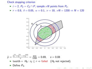
![Define next convex body in MMC
i = 2, P2 = C2 ∩ P, binary search for q ∈ [0.185, 0.28]
r = 0.8, δ = 0.05, α = 0.1, ν = 10, νN = 1200 ⇒ N = 120
q = 0.21, ˆµ =
r
(1)
2 +r
(2)
2 ···+r
(10)
2
ν = 976
1200 = 0.81, s = 0.05
testL→ H0 : r2 ≤ r + δ ⇒ succeed (H0 not rejected).
testR→ H0 : r2 ≤ r ⇒ succeed (H0 rejected).
Set C3 = qC.](https://image.slidesharecdn.com/uoa19-200124130040/85/A-new-practical-algorithm-for-volume-estimation-using-annealing-of-convex-bodies-45-320.jpg)
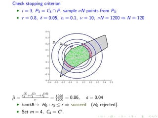
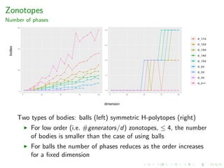
![Convergence criterion
W is a set of n values following Gaussian distribution
Consider the mean value ˆµ, the st.d. s of W and
Pr = m+1
3/4. For each ri assign a value i (is the maximum
allowed error for ri ), s.t. i
2
i = 2.
Using p = (1 + Pr)/2 and the interval [ˆµ − zps, ˆµ + zps]:
if
(ˆµ + zps) − (ˆµ − zps)
ˆµ + zps
=
2zps
ˆµ + zps
≤ i /2, then declare convergence.](https://image.slidesharecdn.com/uoa19-200124130040/85/A-new-practical-algorithm-for-volume-estimation-using-annealing-of-convex-bodies-48-320.jpg)
![Convergence criterion
W is a set of n values following Gaussian distribution
Consider the mean value ˆµ, the st.d. s of W and
Pr = m+1
3/4. For each ri assign a value i (is the maximum
allowed error for ri ), s.t. i
2
i = 2.
Using p = (1 + Pr)/2 and the interval [ˆµ − zps, ˆµ + zps]:
if
(ˆµ + zps) − (ˆµ − zps)
ˆµ + zps
=
2zps
ˆµ + zps
≤ i /2, then declare convergence.
Remark:
If we assume (perfect) uniform sampling from Pi :
1. There is n = O(1) s.t. ri ∈ [ˆµ − zps, ˆµ + zps] with
Pr = m+1
3/4.
2. method estimates vol(P) with probability 3/4 and error ≤ .
In practice it is open how to bound n](https://image.slidesharecdn.com/uoa19-200124130040/85/A-new-practical-algorithm-for-volume-estimation-using-annealing-of-convex-bodies-49-320.jpg)
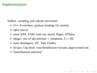
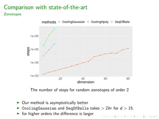
![The volume algorithm
Algorithm 1 VolumeAlgorithm (P, , r, δ, α, ν, N, n)
Construct C ⊆ Rd s.t. C ∩ P = ∅ and set [qmin, qmax]
{P0, . . . , Pm, Cm}=AnnealingSchedule(P, C, r, δ, α, ν, N, qmin, qmax)
m = /2
√
m + 1, = 4(m + 1) − 1/2
√
m + 1
Set i = /
√
m, i = 0, . . . , m − 1
for i = 0, . . . m do
if i < m then
ri = EstimateRatio (Pi , Pi+1, i , m, n)
else
rm = EstimateRatio (Cm, Pm, m, m, n)
end if
end for
return vol(Cm)/r0/ · · · /rm−1 · rm](https://image.slidesharecdn.com/uoa19-200124130040/85/A-new-practical-algorithm-for-volume-estimation-using-annealing-of-convex-bodies-50-320.jpg)
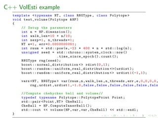
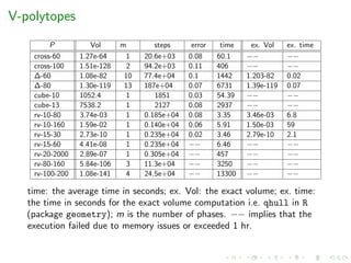
![Zonotopes
Performance
Experimental results for zonotopes.
z-d-k Body order Vol m steps time(sec)
z-5-500 Ball 100 4.63e+13 1 0.1250e+04 22.26
z-20-2000 Ball 100 2.79e+62 1 0.2000e+04 1428
z-50-65 Hpoly 1.3 1.42e+62 1 1.487e+04 173.9
z-100-130 Hpoly 1.3 1.37e+138 3 17.19e+04 6073
z-50-75 Hpoly 1.5 2.96e+66 2 1.615e+04 253.6
z-100-150 Hpoly 1.5 2.32+149 3 15.43e+04 10060
z-70-140 Hpoly 2 8.71e+111 2 5.059e+04 2695
z-100-200 Hpoly 2 5.27e+167 3 15.25e+04 34110
z-d-k: random zonotope in dimension d with k generators;
Body: the type of body used in MMC; m: number of bodies in
MMC
Used to evaluate zonotope approximation methods in
engineering [Kopetzki’17]](https://image.slidesharecdn.com/uoa19-200124130040/85/A-new-practical-algorithm-for-volume-estimation-using-annealing-of-convex-bodies-56-320.jpg)

![Future directions
Better (practical) sampling methods (candidate: Hamiltonian
walk) + implementation
Study convex body families for MMC
Applications:
zonotope approximation in engineering
finance [Cales, Chalkis, Emiris, F, SoCG’18]](https://image.slidesharecdn.com/uoa19-200124130040/85/A-new-practical-algorithm-for-volume-estimation-using-annealing-of-convex-bodies-62-320.jpg)
![Future directions
Better (practical) sampling methods (candidate: Hamiltonian
walk) + implementation
Study convex body families for MMC
Applications:
zonotope approximation in engineering
finance [Cales, Chalkis, Emiris, F, SoCG’18]
Google Summer of Code ’19 call for internships! (contact me :)](https://image.slidesharecdn.com/uoa19-200124130040/85/A-new-practical-algorithm-for-volume-estimation-using-annealing-of-convex-bodies-63-320.jpg)
![Future directions
Better (practical) sampling methods (candidate: Hamiltonian
walk) + implementation
Study convex body families for MMC
Applications:
zonotope approximation in engineering
finance [Cales, Chalkis, Emiris, F, SoCG’18]
Google Summer of Code ’19 call for internships! (contact me :)](https://image.slidesharecdn.com/uoa19-200124130040/85/A-new-practical-algorithm-for-volume-estimation-using-annealing-of-convex-bodies-64-320.jpg)

The document presents a new annealing schedule method for estimating the volume of convex polytopes in Rd by utilizing a sequence of convex bodies and applying statistical t-tests for volume ratios. It highlights various computational complexities in volume estimation and introduces methodologies including multiphase Monte Carlo sampling techniques. Additionally, it discusses efficient algorithms, limitations, and applications of volume computations in areas such as autonomous driving and bio-geography.


![Polymer [ बहुलक ] Chemistry Notes PDF - Irfanullah Mehar - JJ Sir Chemistry.pdf](https://cdn.slidesharecdn.com/ss_thumbnails/polymerchemistrynotespdf-irfanullahmehar-jjsirchemistry-260210172118-3f9b37f7-thumbnail.jpg?width=640&height=640&fit=bounds)


