Practical volume estimation by a new annealing
schedule for cooling convex bodies
A.Chalkis, I.Z.Emiris, V. Fisikopoulos
Dept. of Informatics & Telecommunications, University of Athens
Volume computation
Given P a convex polytope in Rd compute the volume of P.
Volume computation
Given P a convex polytope in Rd compute the volume of P.
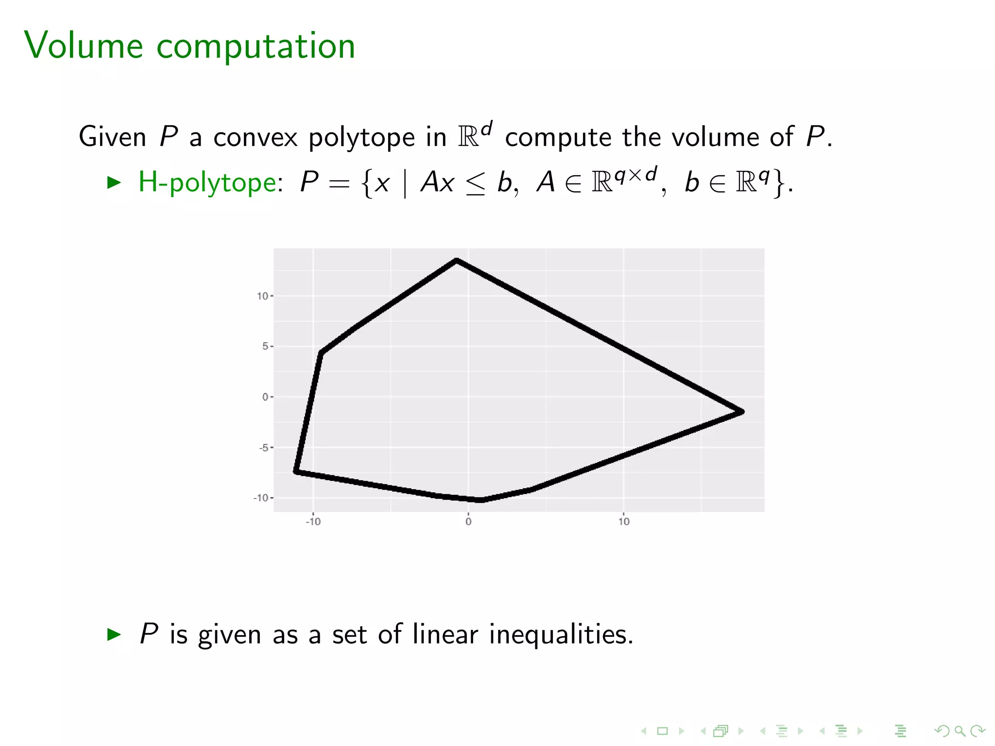
H-polytope: P = {x | Ax ≤ b, A ∈ Rq×d , b ∈ Rq}.
Volume computation
Given P a convex polytope in Rd compute the volume of P.
H-polytope: P = {x | Ax ≤ b, A ∈ Rq×d , b ∈ Rq}.
P is given as a set of linear inequalities.
Our setting
Given P a convex polytope in Rd compute the volume of P.
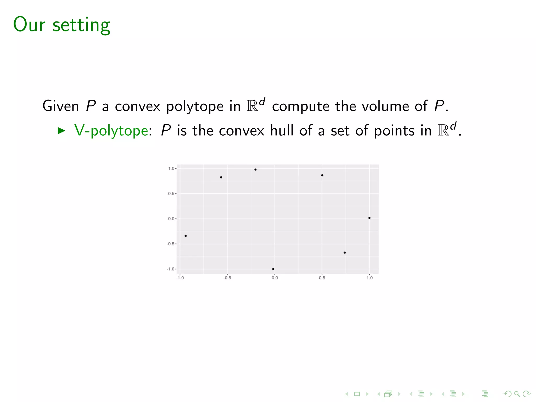
V-polytope: P is the convex hull of a set of points in Rd .
Our setting
Given P a convex polytope in Rd compute the volume of P.
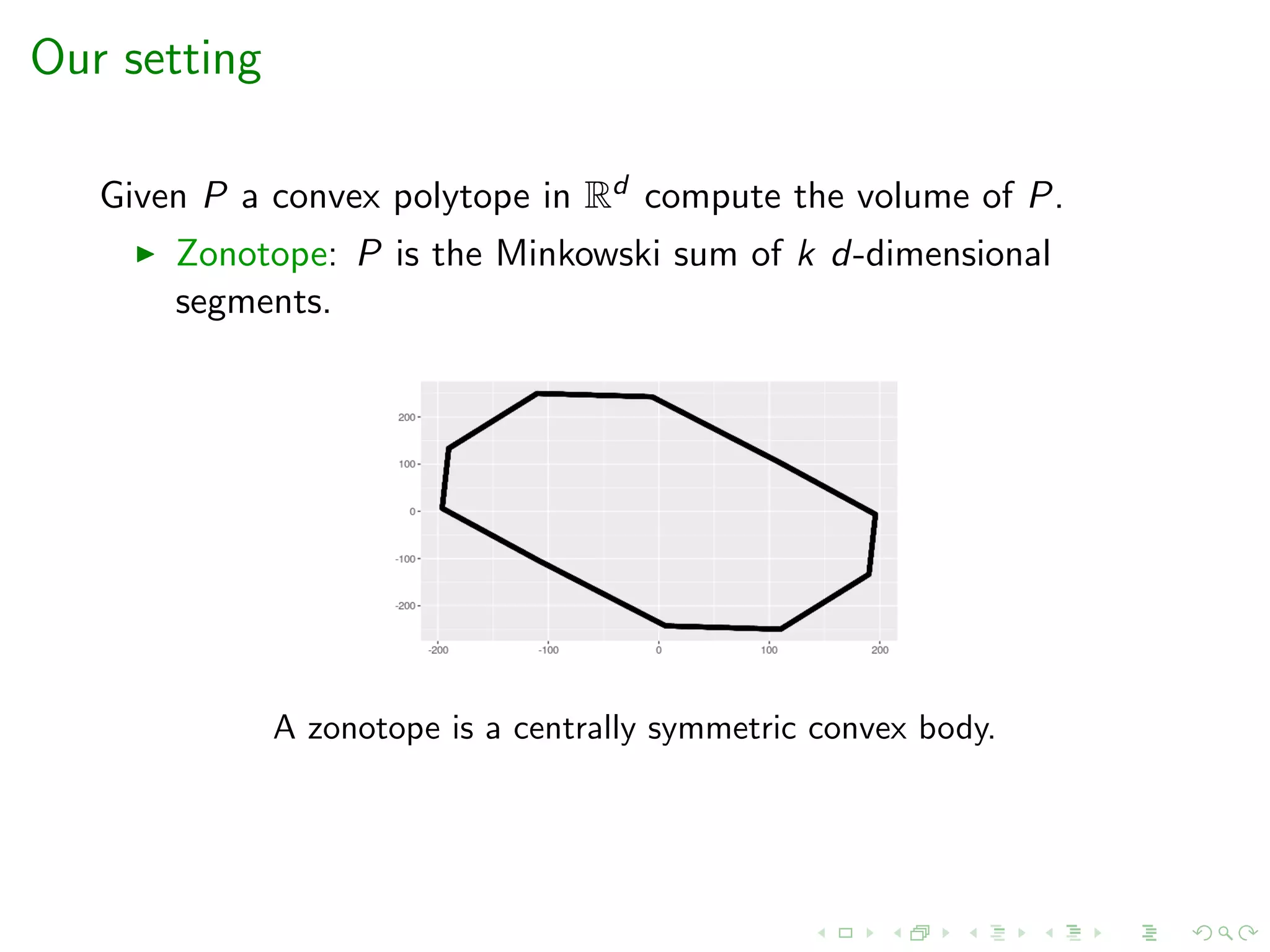
Zonotope: P is the Minkowski sum of k d-dimensional
segments.
A zonotope is a centrally symmetric convex body.
Complexity
Computing the exact volume of P,
Complexity
Computing the exact volume of P,
is #P-hard for all the representations [DyerFrieze’88]
Complexity
Computing the exact volume of P,
is #P-hard for all the representations [DyerFrieze’88]
is open if both H- and V- representations available
Complexity
Computing the exact volume of P,
is #P-hard for all the representations [DyerFrieze’88]
is open if both H- and V- representations available
is APX-hard (oracle model) [Elekes’86]
Our goal
A new practical volume estimation for V-polytopes and
zonotopes.
Our goal
A new practical volume estimation for V-polytopes and
zonotopes.
Why:
Volume computation of such polytopes appear in engineering
and data science.
Current state-of-the-art software can not scale beyond, say
d ≥ 15.
Randomized algorithms
Theorem
For any convex body K and any 0 ≤ , δ ≤ 1, there is a
randomized algorithm which computes an estimate V s.t. with
probability 1 − δ we have (1 − )vol(K) ≤ V ≤ (1 + )vol(K), and
the number of oracle calls is poly(d, 1/ , log(1/δ)).
Using randomness, we can go from an exponential
approximation to an arbitrarily small one.
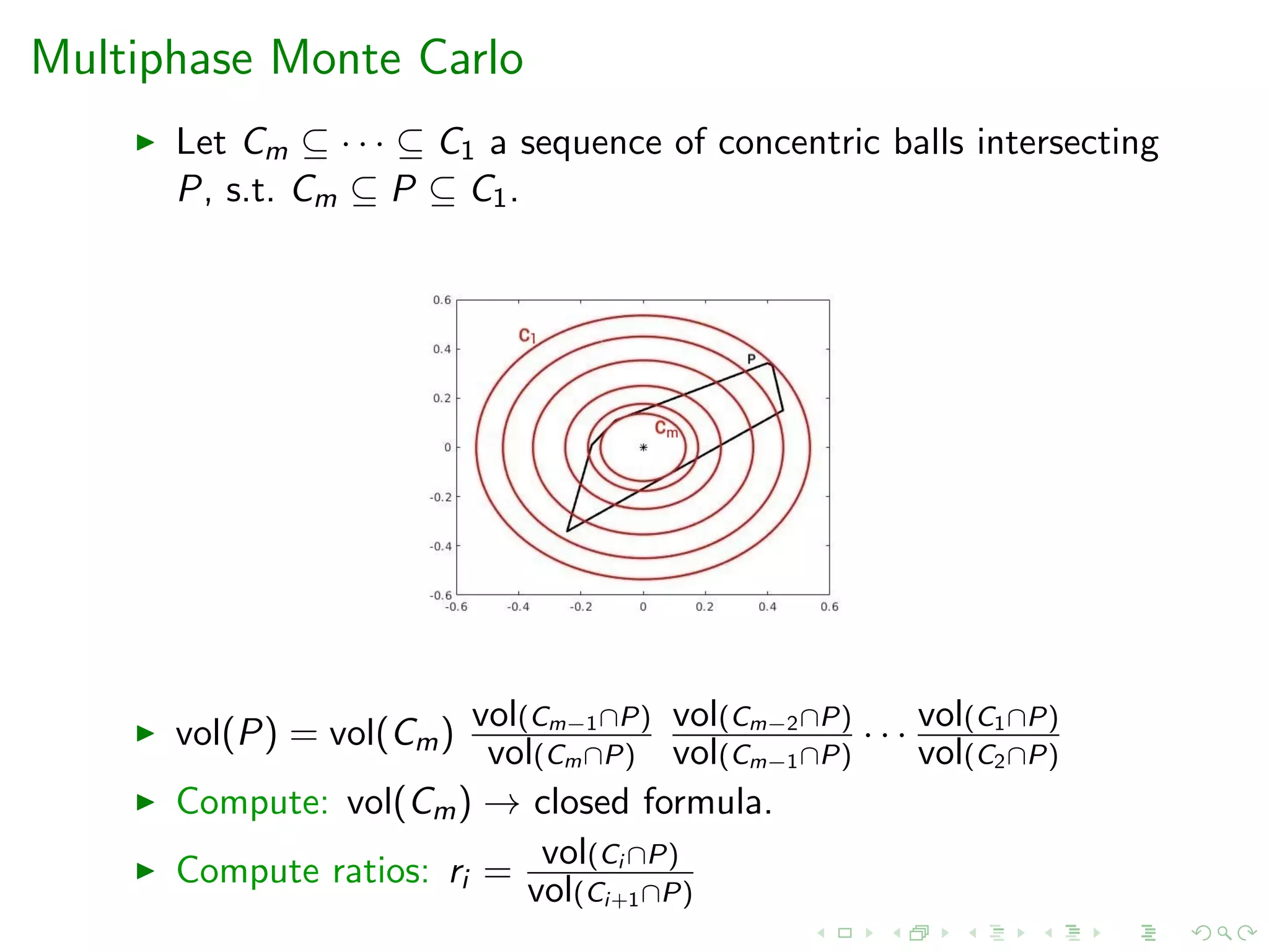
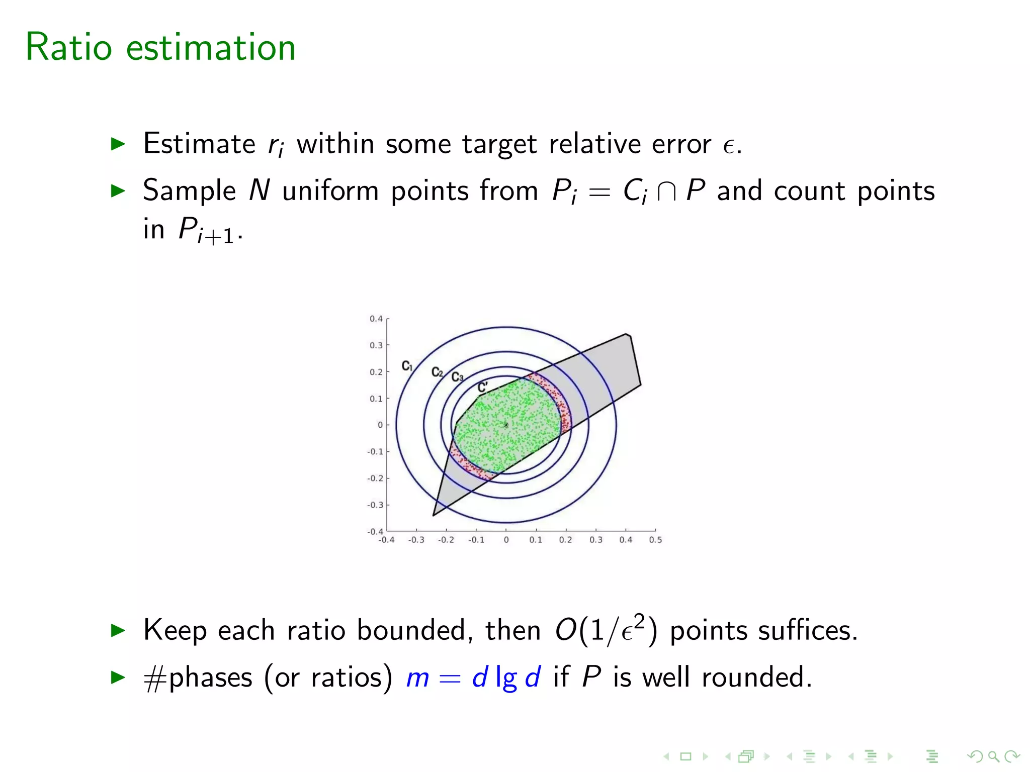
Multiphase Monte Carlo
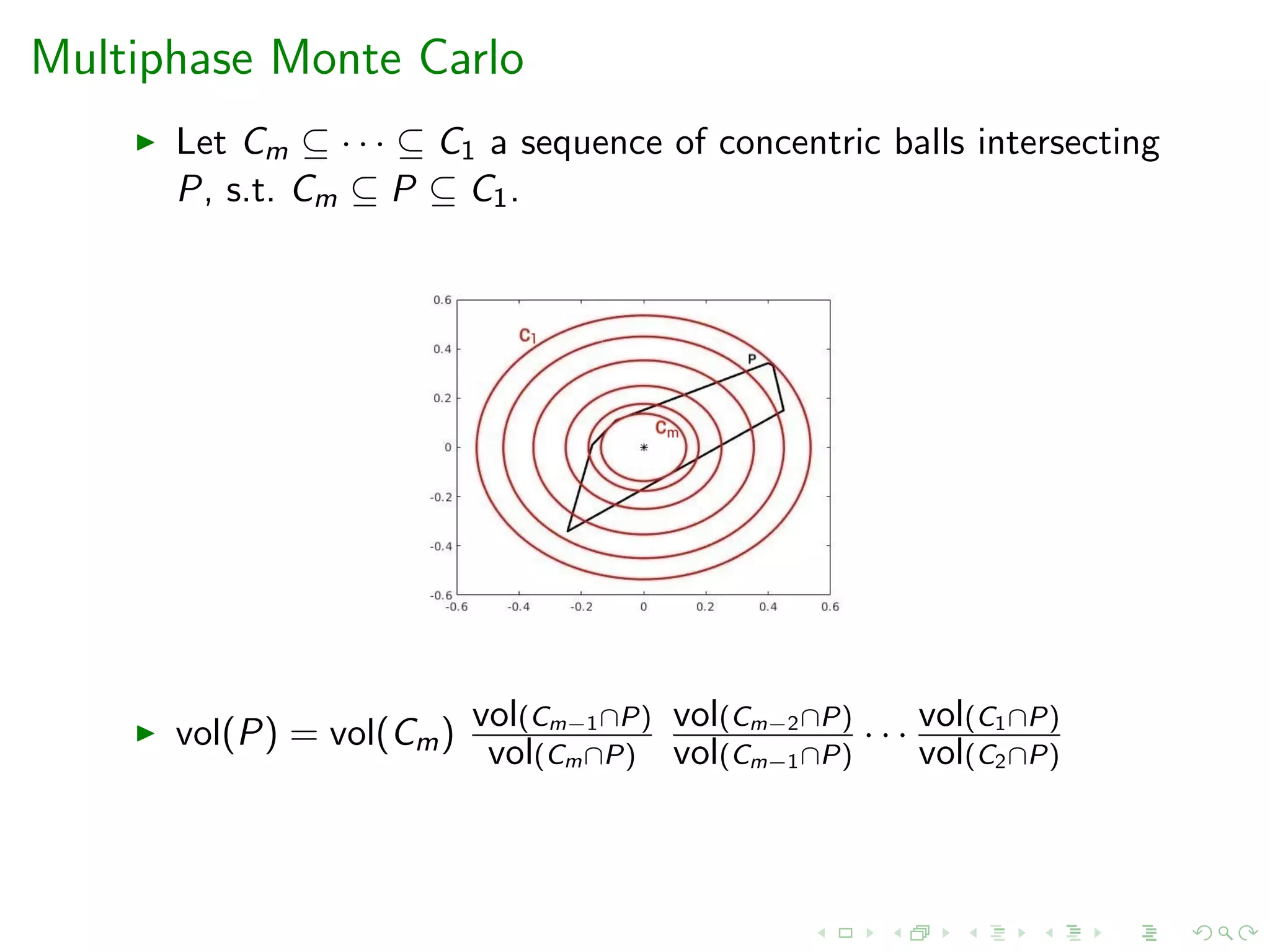
Let Cm ⊆ · · · ⊆ C1 a sequence of concentric balls intersecting
P, s.t. Cm ⊆ P ⊆ C1.
Multiphase Monte Carlo
Let Cm ⊆ · · · ⊆ C1 a sequence of concentric balls intersecting
P, s.t. Cm ⊆ P ⊆ C1.
vol(P) = vol(Cm) vol(Cm−1∩P)
vol(Cm∩P)
vol(Cm−2∩P)
vol(Cm−1∩P)
· · · vol(C1∩P)
vol(C2∩P)
Multiphase Monte Carlo
Let Cm ⊆ · · · ⊆ C1 a sequence of concentric balls intersecting
P, s.t. Cm ⊆ P ⊆ C1.
vol(P) = vol(Cm) vol(Cm−1∩P)
vol(Cm∩P)
vol(Cm−2∩P)
vol(Cm−1∩P)
· · · vol(C1∩P)
vol(C2∩P)
Compute: vol(Cm) → closed formula.
Multiphase Monte Carlo
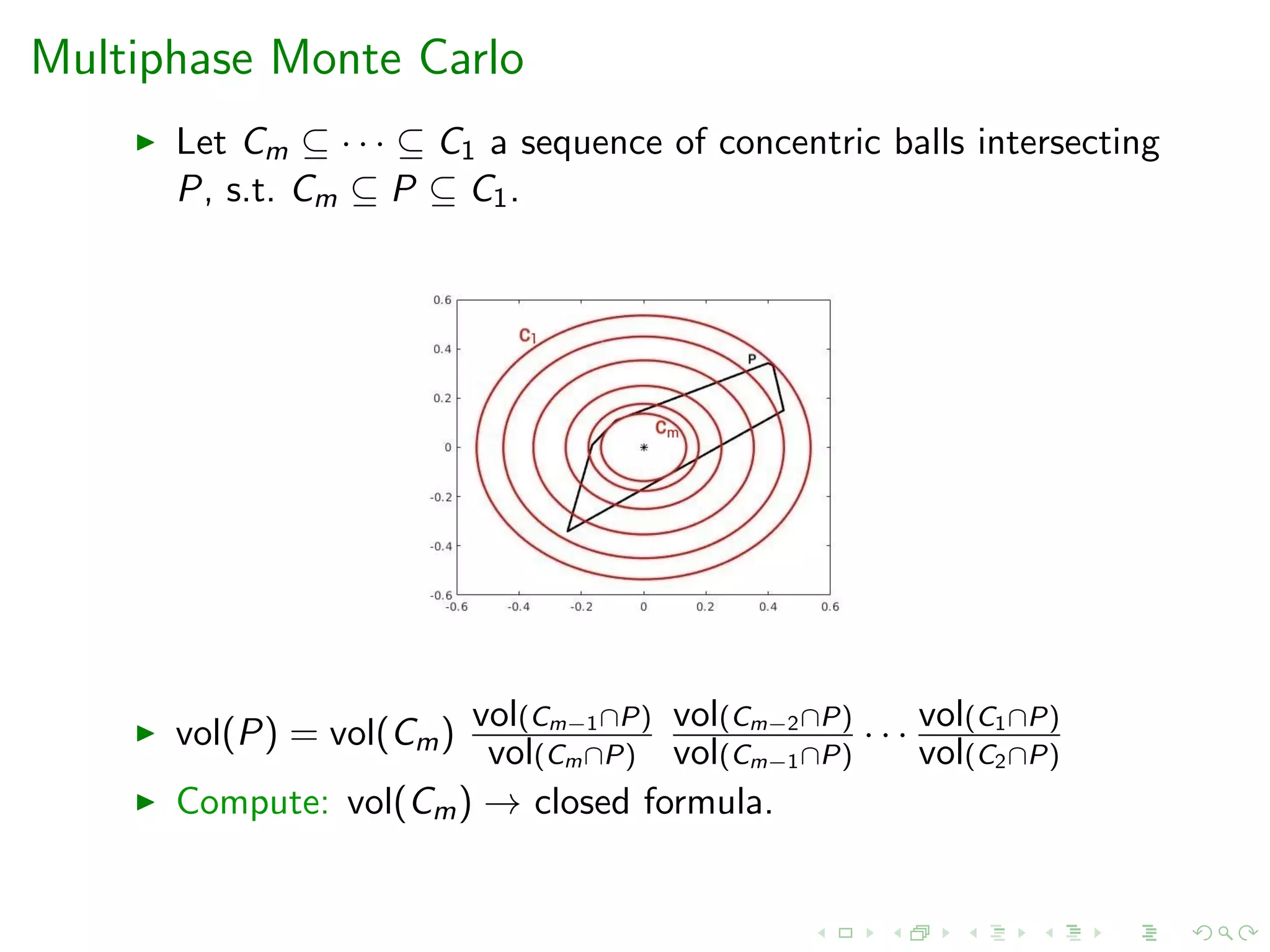
Let Cm ⊆ · · · ⊆ C1 a sequence of concentric balls intersecting
P, s.t. Cm ⊆ P ⊆ C1.
vol(P) = vol(Cm) vol(Cm−1∩P)
vol(Cm∩P)
vol(Cm−2∩P)
vol(Cm−1∩P)
· · · vol(C1∩P)
vol(C2∩P)
Compute: vol(Cm) → closed formula.
Compute ratios: ri = vol(Ci ∩P)
vol(Ci+1∩P)
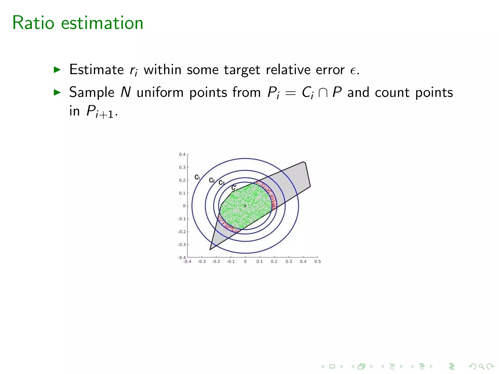
Ratio estimation
Estimate ri within some target relative error .
Ratio estimation
Estimate ri within some target relative error .
Sample N uniform points from Pi = Ci ∩ P and count points
in Pi+1.
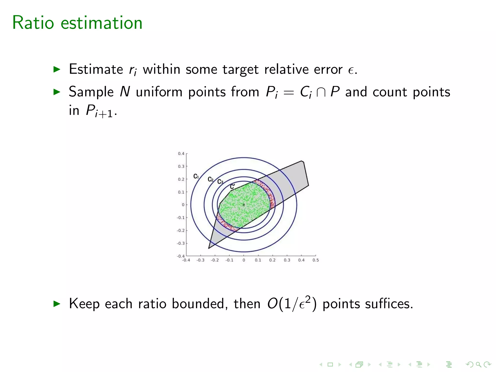
Ratio estimation
Estimate ri within some target relative error .
Sample N uniform points from Pi = Ci ∩ P and count points
in Pi+1.
Keep each ratio bounded, then O(1/ 2) points suffices.
Ratio estimation
Estimate ri within some target relative error .
Sample N uniform points from Pi = Ci ∩ P and count points
in Pi+1.
Keep each ratio bounded, then O(1/ 2) points suffices.
#phases (or ratios) m = d lg d if P is well rounded.
Sampling
To sample uniformly distributed points from Pi we use
geometric random walks (Markov chain).
Sampling
To sample uniformly distributed points from Pi we use
geometric random walks (Markov chain).
A geometric r.w. starts at p0 ∈ P and at each step i, moves to
a ”neighboring” point pi+1 that depends only on pi .
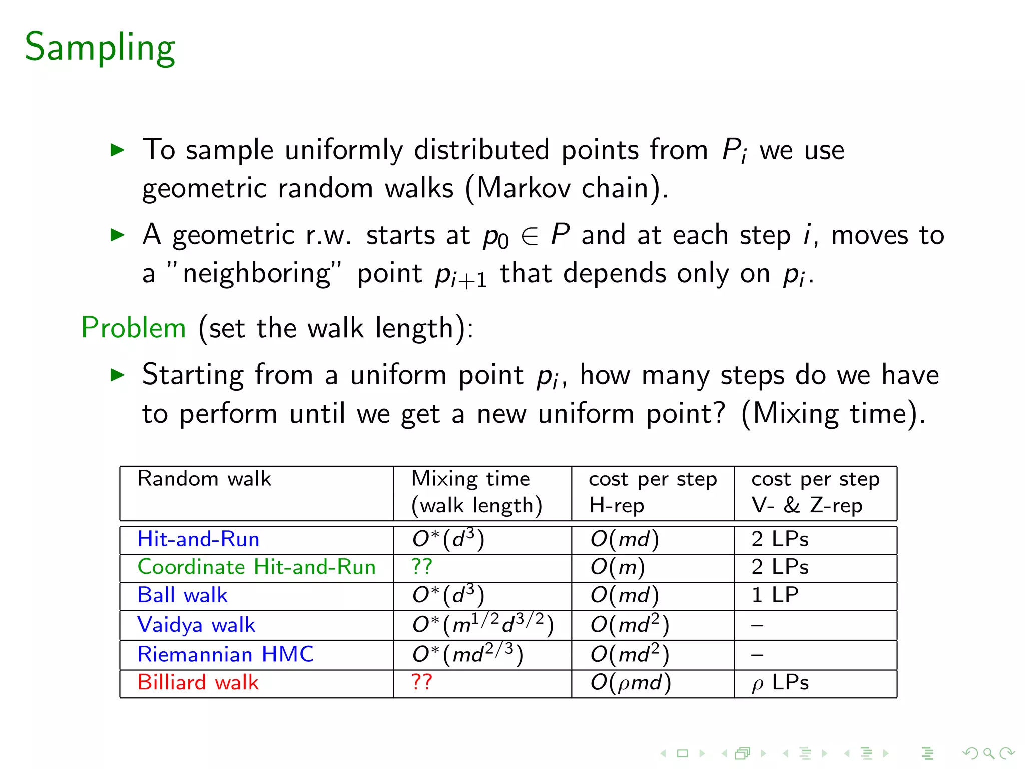
Problem (set the walk length):
Starting from a uniform point pi , how many steps do we have
to perform until we get a new uniform point? (Mixing time).
Random walk Mixing time cost per step cost per step
(walk length) H-rep V- & Z-rep
Hit-and-Run O∗(d3) O(md) 2 LPs
Coordinate Hit-and-Run ?? O(m) 2 LPs
Ball walk O∗(d3) O(md) 1 LP
Vaidya walk O∗(m1/2d3/2) O(md2) –
Riemannian HMC O∗(md2/3) O(md2) –
Billiard walk ?? O(ρmd) ρ LPs
Sampling
Random walk Mixing time cost per step cost per step
(number of steps) H-rep V- & Z-rep
Coordinate Hit-and-Run ?? O(m) 2 LPs
Billiard walk ?? O(ρmd) ρ LPs
Coordinate Hit-and-Run:
Is the main paradigm in applications and software.
In practice converges to uniform distribution in O(d2) steps
[Cousins, Vempala’17].
Billiard walk:
Converges faster to uniform distribution than Hit-and-Run in
practice [Polyak’14].
For V-polytopes and zonotopes has comparable cost per step
with Coordinate Hit-and-Run.
Billiard walk
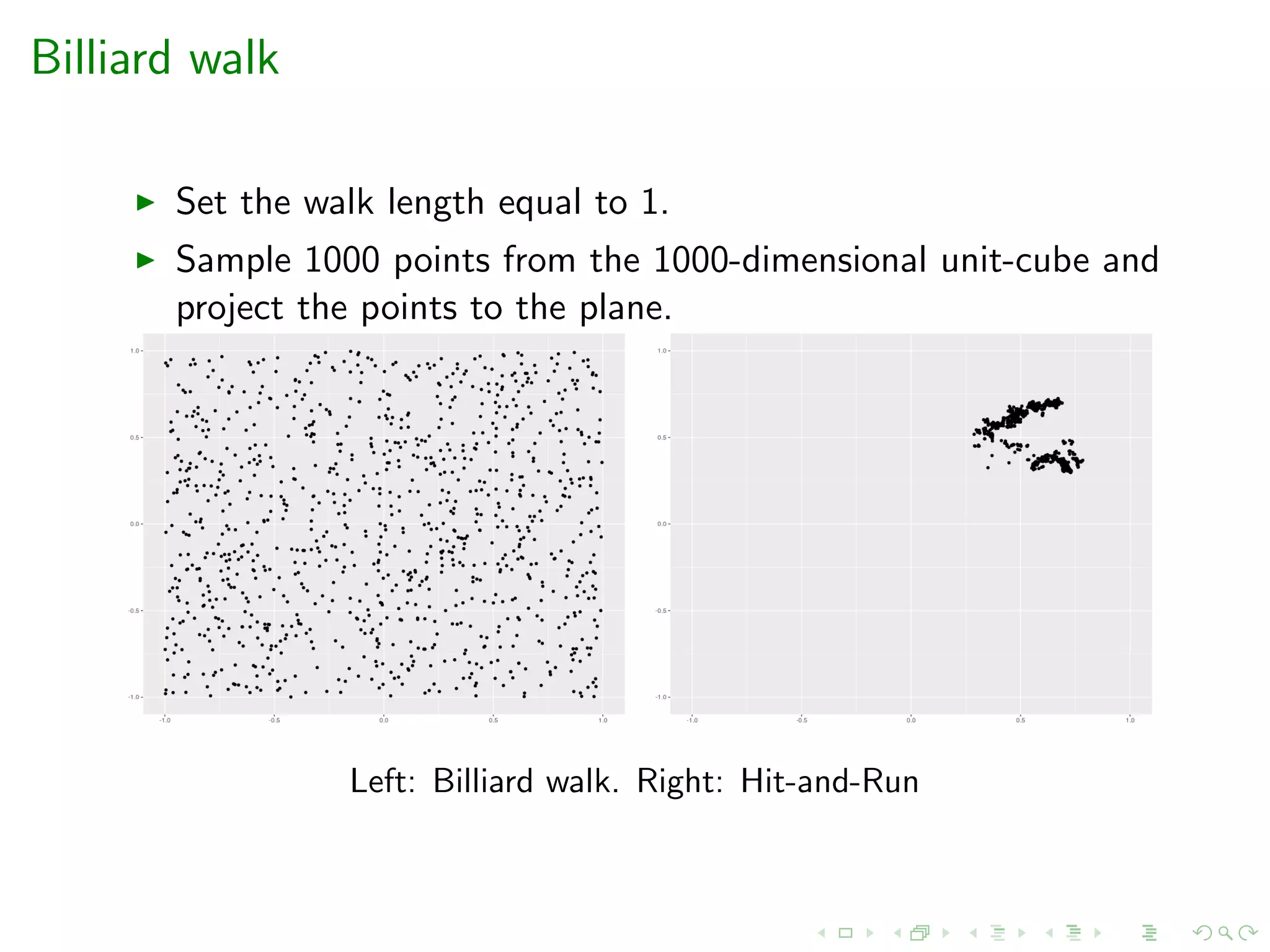
Set the walk length equal to 1.
Sample 1000 points from the 1000-dimensional unit-cube and
project the points to the plane.
Left: Billiard walk. Right: Hit-and-Run
State-of-the-art
Authors-Year Complexity Algorithm
(oracle calls)
[Dyer, Frieze, Kannan’91] O∗(d23) Sequence of balls + grid walk
[Kannan, Lovasz, Simonovits’97] O∗(d5) Sequence of balls + ball walk
[Lovasz, Vempala’03] O∗(d4) Exponential dist. + hit-and-run
[Cousins, Vempala’15] O∗(d3) Spherical Gaussians + ball walk
Practical methods:
Follow theory but make practical adjustments (experimental).
[Emiris, F’14] Sequence of balls + coordinate hit-and-run.
[Cousins, Vempala’16] Spherical Gaussians + coordinate
hit-and-run
Limitations
Limitations of existing practical methods:
Efficient only for H-polytopes (scale up-to few hundred dims in
hrs)
Limitations
Limitations of existing practical methods:
Efficient only for H-polytopes (scale up-to few hundred dims in
hrs)
For V-polytopes or zonotopes:
Both of them request an inscribed ball (ideally the maximum)
C ⊆ P.
The number of total steps is strongly determined by the radius
of C.
[Cousins, Vempala’16] needs a bound on the number of facets.
Our contributions
Multiphase Monte Carlo: We allow any convex body C (that
”fits well” to P and is ”easy” to sample from) besides ball to
construct the sequence.
Our contributions
Multiphase Monte Carlo: We allow any convex body C (that
”fits well” to P and is ”easy” to sample from) besides ball to
construct the sequence.
Sampling: Billiard walk to V-polytopes and zonotopes.
Our contributions
Multiphase Monte Carlo: We allow any convex body C (that
”fits well” to P and is ”easy” to sample from) besides ball to
construct the sequence.
Sampling: Billiard walk to V-polytopes and zonotopes.
A new simulated annealing method to construct a sparser
sequence of bodies.
Sequence by [L.S.’97] (left) and by annealing schedule (right).
Our method can be easily extended for any polytope P that is
given as a projection of a polytope Q.
Annealing Schedule
Inputs: Polytope P, body C, cooling parameters r, δ > 0.
Output: A sequence of scaled copies of C, Cm ⊆ · · · ⊆ C1 s.t.
vol(Pi+1)/vol(Pi ) ∈ [r, r + δ] with high probability
where Pi = Ci ∩ P, i = 1, . . . , m and P0 = P.
Statistical tests
for the ratio of volumes of convex bodies
Given convex bodies Pi ⊇ Pi+1, we define two statistical tests:
testL(Pi , Pi+1, r, δ): testR(Pi , Pi+1, r, δ):
H0 : vol(Pi+1)/vol(Pi ) ≥ r + δ H0 : vol(Pi+1)/vol(Pi ) ≤ r
Successful if we reject H0 Successful if we reject H0
If both testL and testR are successful then
ri = vol(Pi+1)/vol(Pi ) ∈ [r, r + δ], with high probability.
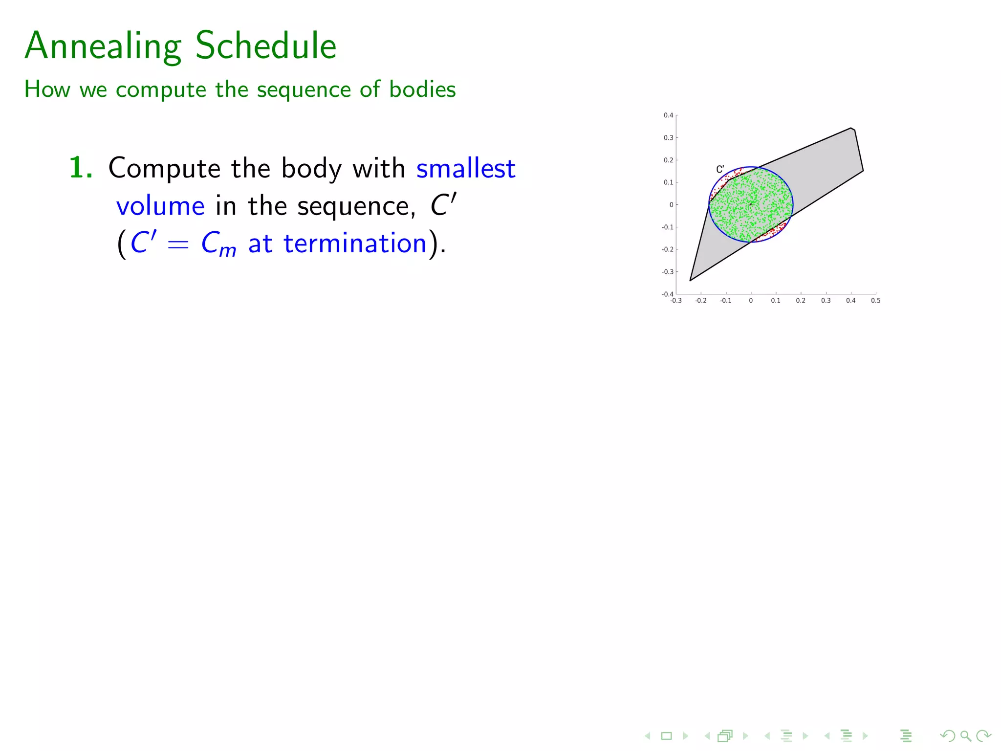
Annealing Schedule
How we compute the sequence of bodies
1. Compute the body with smallest
volume in the sequence, C
(C = Cm at termination).
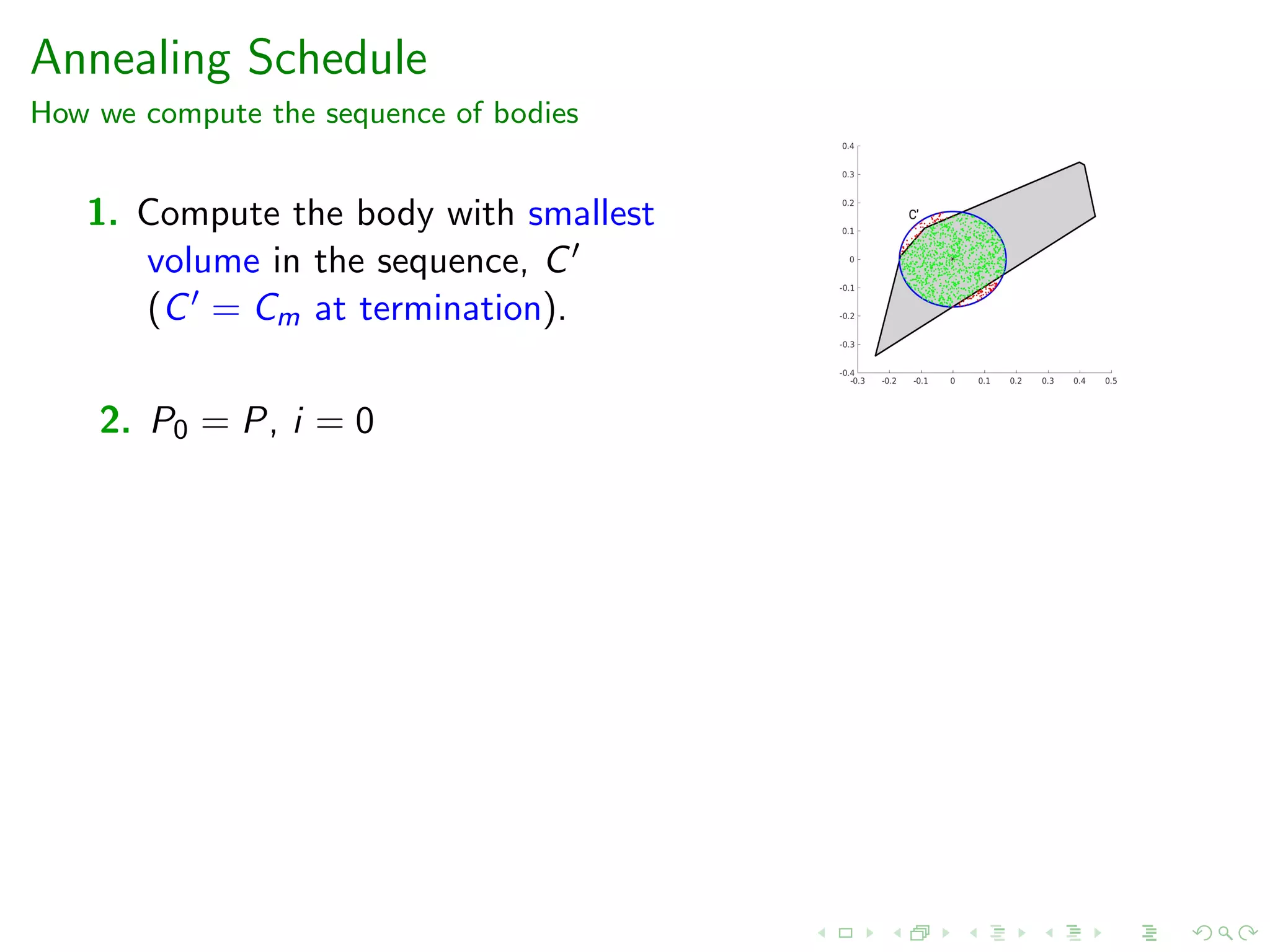
Annealing Schedule
How we compute the sequence of bodies
1. Compute the body with smallest
volume in the sequence, C
(C = Cm at termination).
2. P0 = P, i = 0
Annealing Schedule
How we compute the sequence of bodies
1. Compute the body with smallest
volume in the sequence, C
(C = Cm at termination).
2. P0 = P, i = 0
3. if vol(C ∩ P)/vol(Pi ) ≥ r set m = i + 1, Cm = C stop
otherwise construct Pi+1 s.t. vol(Pi+1)/vol(Pi ) ∈ [r, r + δ].
Check stopping criterion Construct Pi+1
4. i = i + 1, return to step 3.
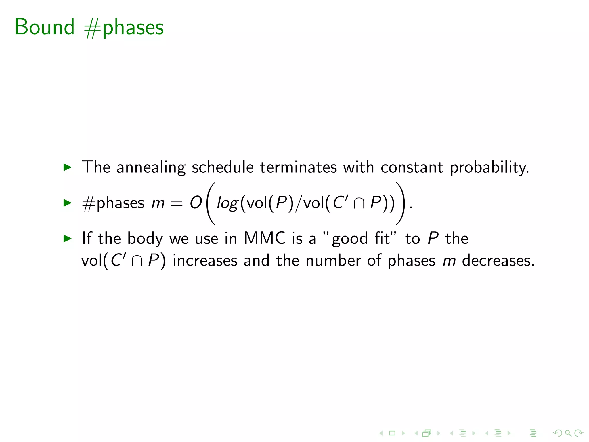
Bound #phases
The annealing schedule terminates with constant probability.
#phases m = O log(vol(P)/vol(C ∩ P)) .
If the body we use in MMC is a ”good fit” to P the
vol(C ∩ P) increases and the number of phases m decreases.
Zonotopes
Number of phases
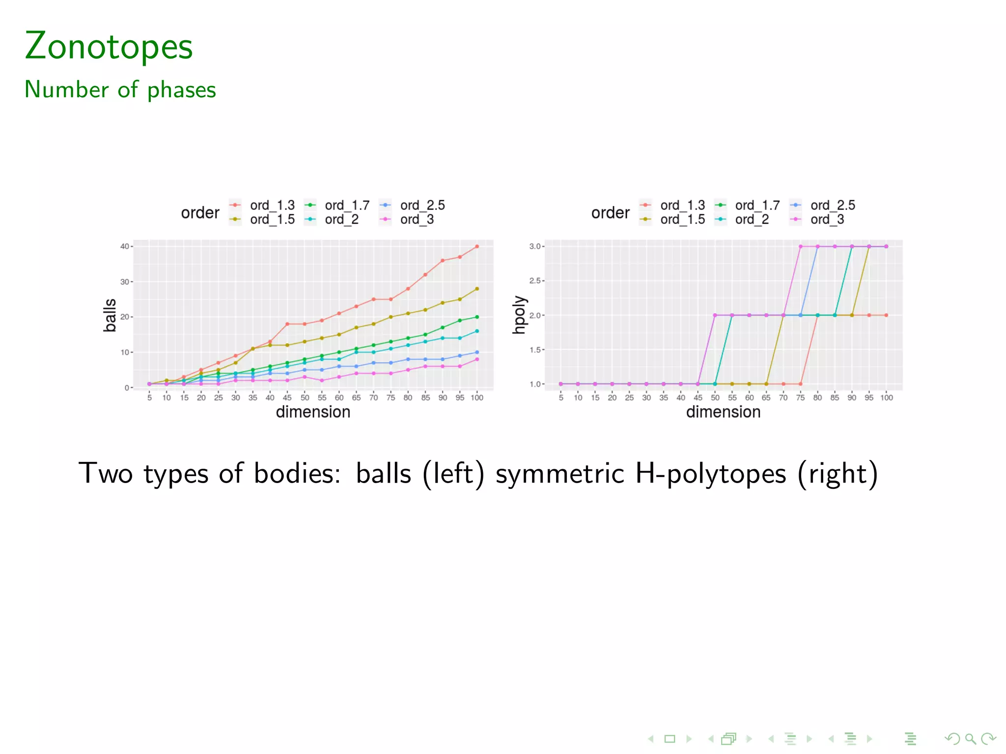
We use the generators of the zonotope P in order to define a
centrally symmetric H-polytope that is a ”good fit” to P.
In both figures vol(C ∩ P)/vol(C ) ∈ [0.8, 0.85].
Zonotopes
Number of phases
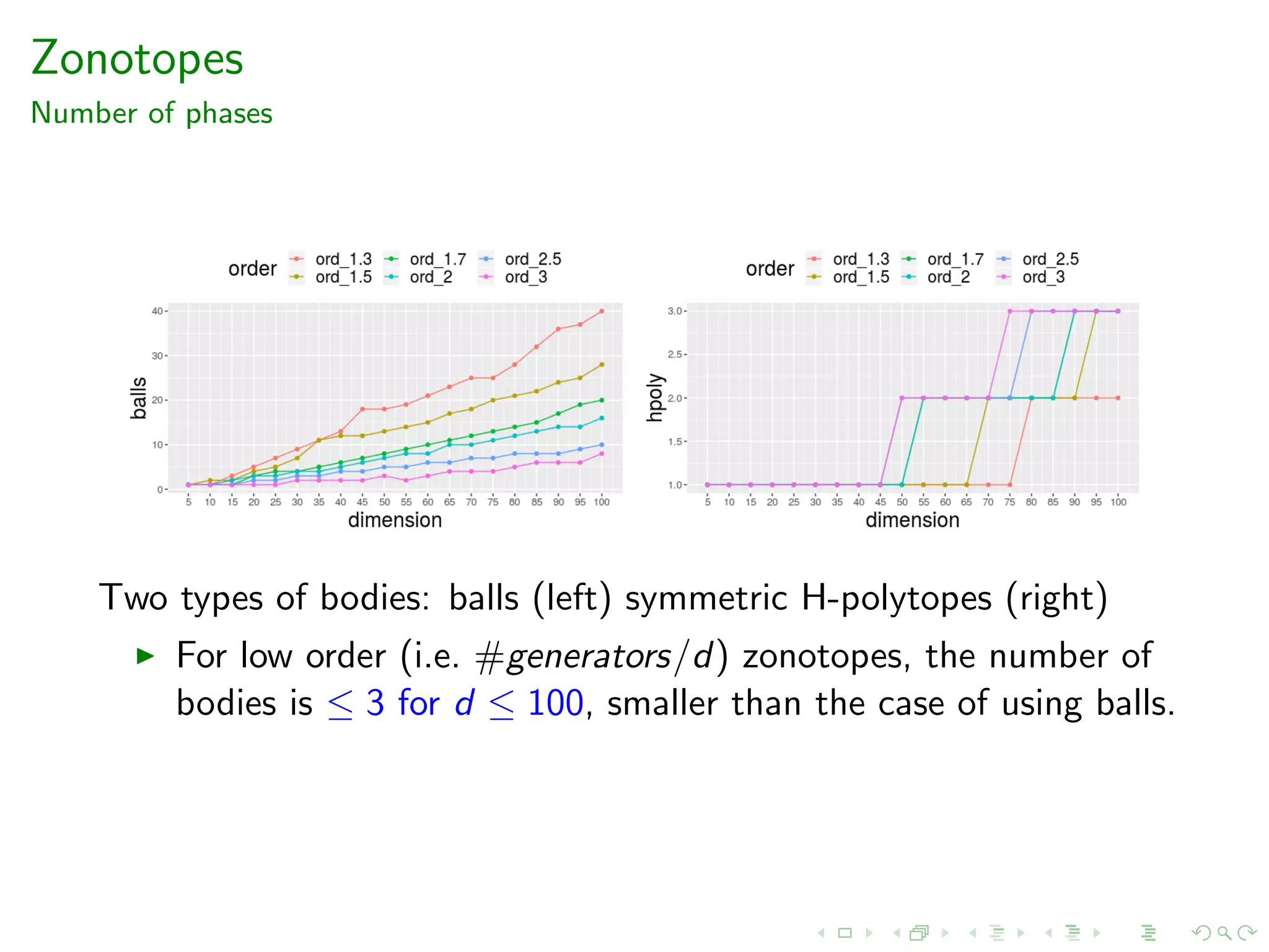
Two types of bodies: balls (left) symmetric H-polytopes (right)
Zonotopes
Number of phases
Two types of bodies: balls (left) symmetric H-polytopes (right)
For low order (i.e. #generators/d) zonotopes, the number of
bodies is ≤ 3 for d ≤ 100, smaller than the case of using balls.
Zonotopes
Number of phases
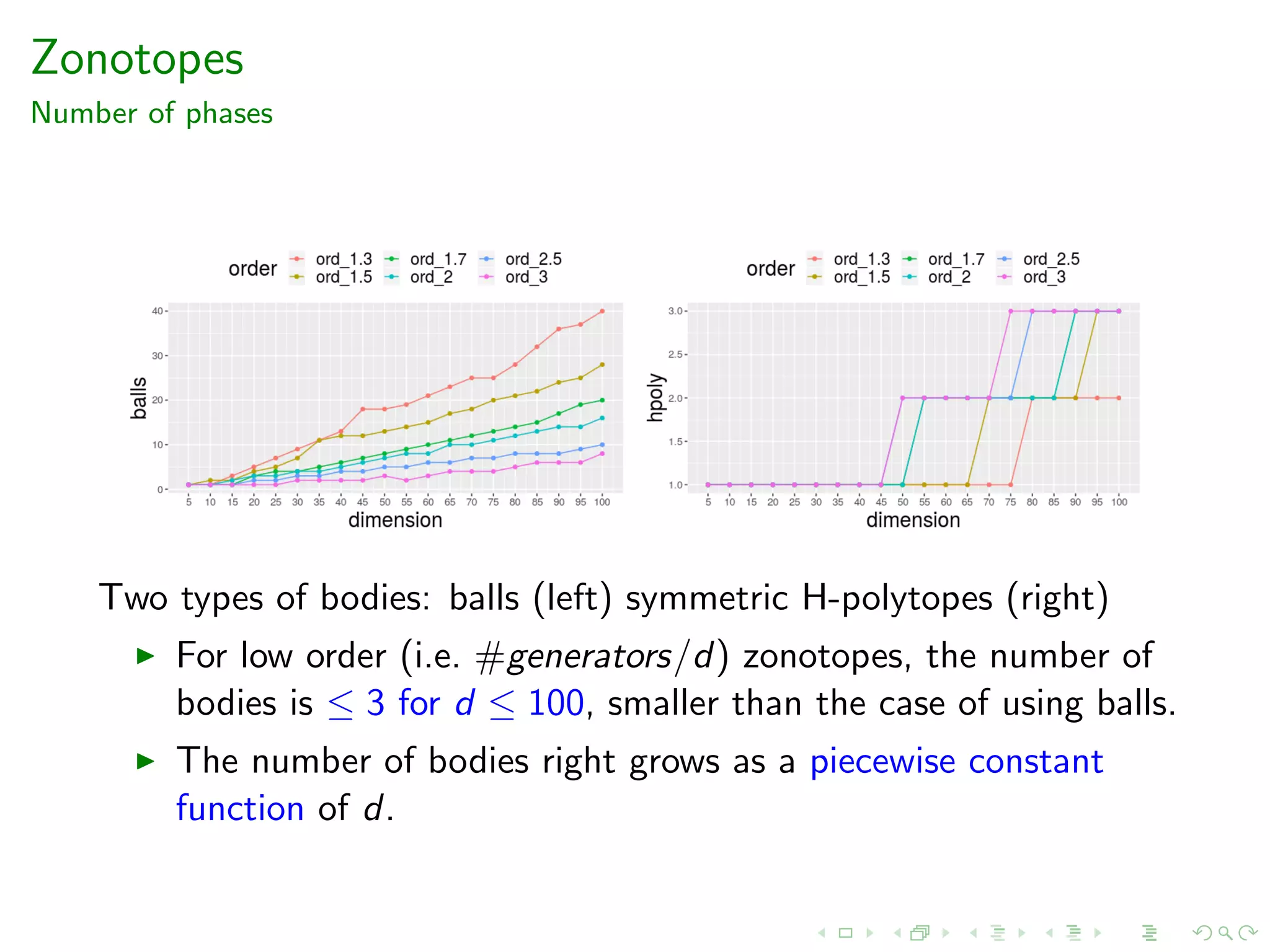
Two types of bodies: balls (left) symmetric H-polytopes (right)
For low order (i.e. #generators/d) zonotopes, the number of
bodies is ≤ 3 for d ≤ 100, smaller than the case of using balls.
The number of bodies right grows as a piecewise constant
function of d.
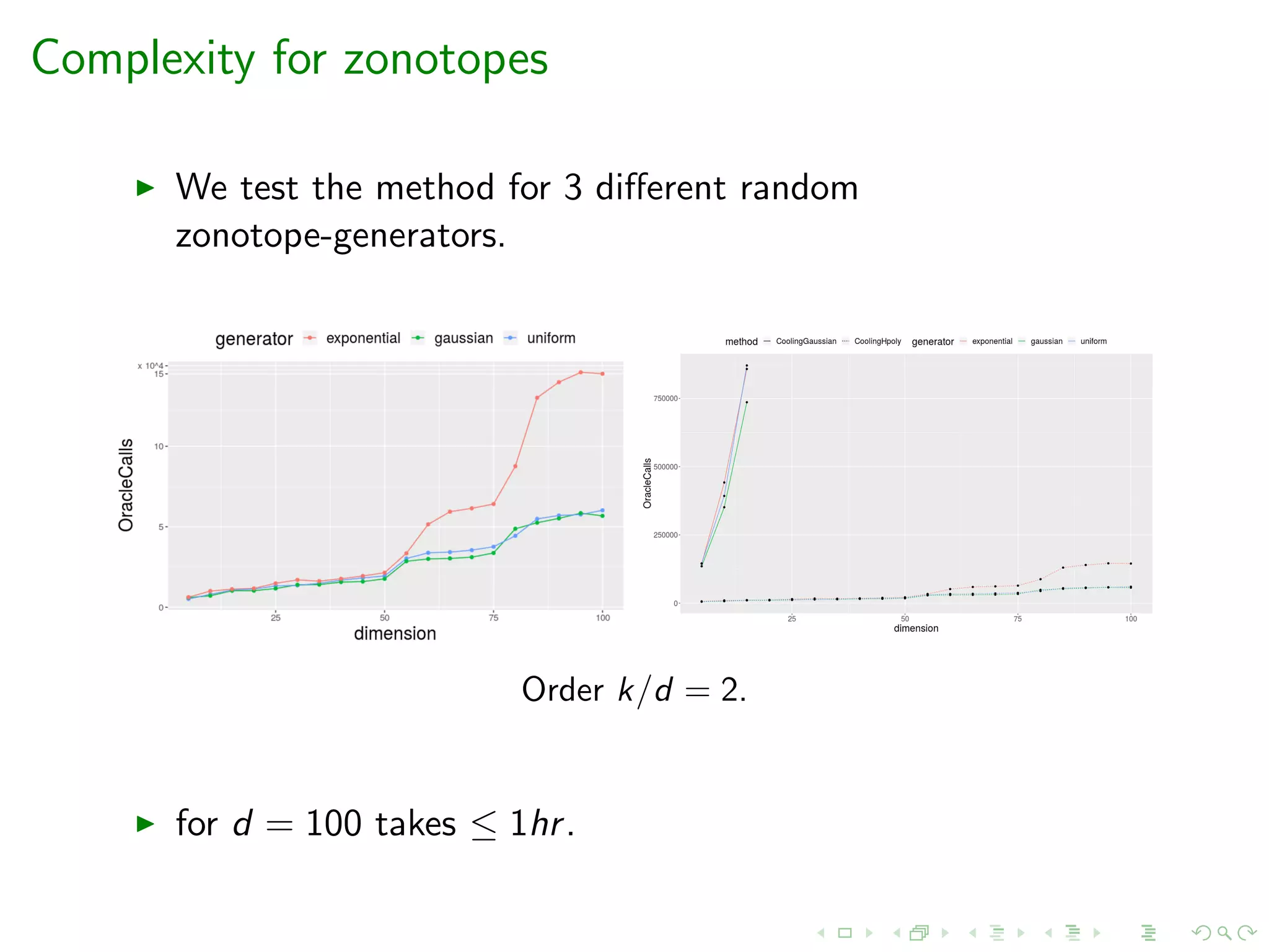
Complexity for zonotopes
We test the method for 3 different random
zonotope-generators.
Order k/d = 2.
for d = 100 takes ≤ 1hr.
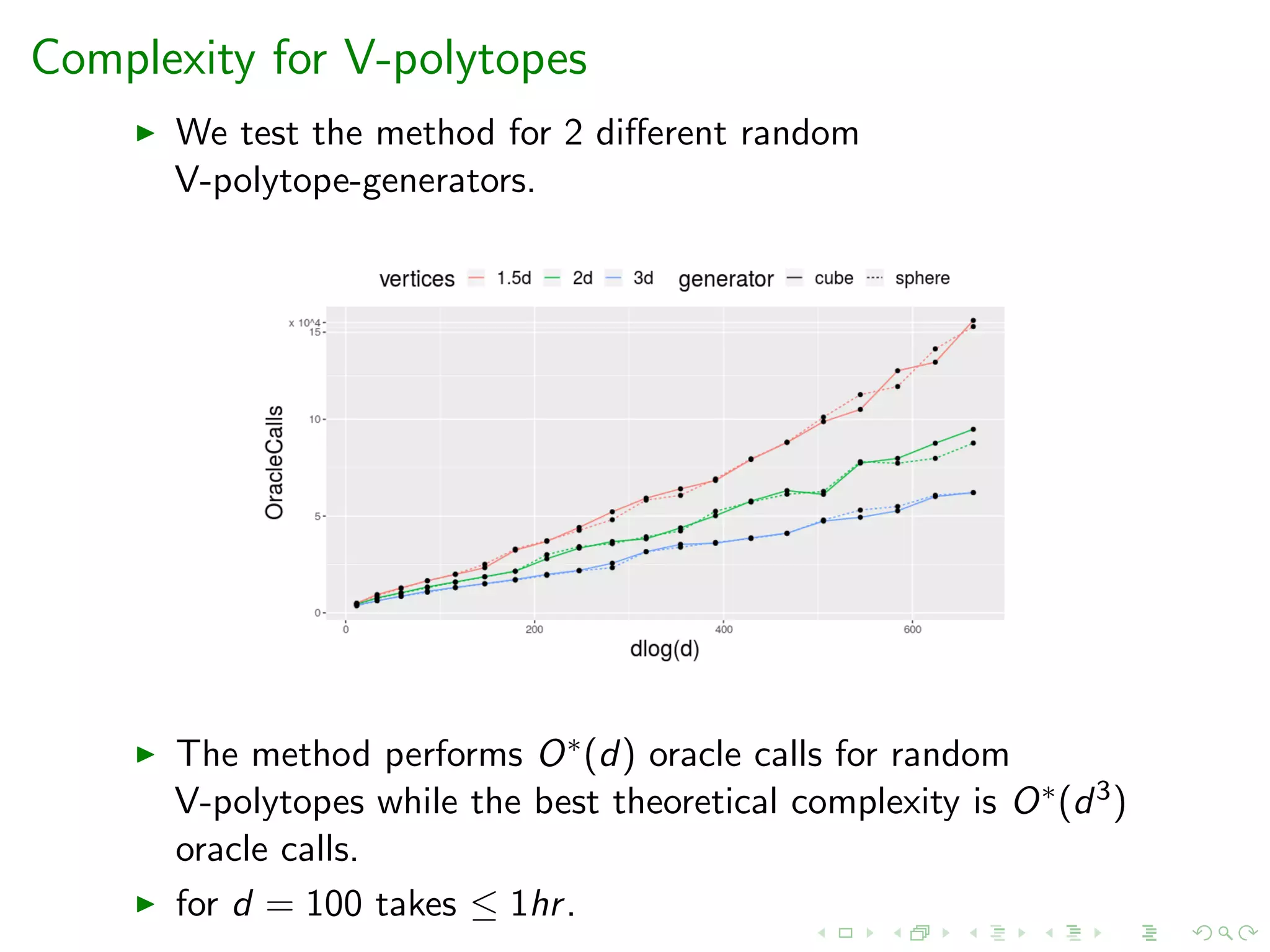
Complexity for V-polytopes
We test the method for 2 different random
V-polytope-generators.
The method performs O∗(d) oracle calls for random
V-polytopes while the best theoretical complexity is O∗(d3)
oracle calls.
for d = 100 takes ≤ 1hr.
Supported by Google Summer of Code 2018 and 2019.
The implementations in C++ are included to the R package
volesti1 in CRAN.
More development branches in Github2.
1
https://cran.r-project.org/web/packages/volesti/index.html
2
https://github.com/GeomScale/volume_approximation

14th Athens Colloquium on Algorithms and Complexity (ACAC19)

  • 1.
    Practical volume estimationby a new annealing schedule for cooling convex bodies A.Chalkis, I.Z.Emiris, V. Fisikopoulos Dept. of Informatics & Telecommunications, University of Athens
  • 2.
    Volume computation Given Pa convex polytope in Rd compute the volume of P.
  • 3.
    Volume computation Given Pa convex polytope in Rd compute the volume of P. H-polytope: P = {x | Ax ≤ b, A ∈ Rq×d , b ∈ Rq}.
  • 4.
    Volume computation Given Pa convex polytope in Rd compute the volume of P. H-polytope: P = {x | Ax ≤ b, A ∈ Rq×d , b ∈ Rq}. P is given as a set of linear inequalities.
  • 5.
    Our setting Given Pa convex polytope in Rd compute the volume of P. V-polytope: P is the convex hull of a set of points in Rd .
  • 6.
    Our setting Given Pa convex polytope in Rd compute the volume of P. Zonotope: P is the Minkowski sum of k d-dimensional segments. A zonotope is a centrally symmetric convex body.
  • 7.
  • 8.
    Complexity Computing the exactvolume of P, is #P-hard for all the representations [DyerFrieze’88]
  • 9.
    Complexity Computing the exactvolume of P, is #P-hard for all the representations [DyerFrieze’88] is open if both H- and V- representations available
  • 10.
    Complexity Computing the exactvolume of P, is #P-hard for all the representations [DyerFrieze’88] is open if both H- and V- representations available is APX-hard (oracle model) [Elekes’86]
  • 11.
    Our goal A newpractical volume estimation for V-polytopes and zonotopes.
  • 12.
    Our goal A newpractical volume estimation for V-polytopes and zonotopes. Why: Volume computation of such polytopes appear in engineering and data science. Current state-of-the-art software can not scale beyond, say d ≥ 15.
  • 13.
    Randomized algorithms Theorem For anyconvex body K and any 0 ≤ , δ ≤ 1, there is a randomized algorithm which computes an estimate V s.t. with probability 1 − δ we have (1 − )vol(K) ≤ V ≤ (1 + )vol(K), and the number of oracle calls is poly(d, 1/ , log(1/δ)). Using randomness, we can go from an exponential approximation to an arbitrarily small one.
  • 14.
    Multiphase Monte Carlo LetCm ⊆ · · · ⊆ C1 a sequence of concentric balls intersecting P, s.t. Cm ⊆ P ⊆ C1.
  • 15.
    Multiphase Monte Carlo LetCm ⊆ · · · ⊆ C1 a sequence of concentric balls intersecting P, s.t. Cm ⊆ P ⊆ C1. vol(P) = vol(Cm) vol(Cm−1∩P) vol(Cm∩P) vol(Cm−2∩P) vol(Cm−1∩P) · · · vol(C1∩P) vol(C2∩P)
  • 16.
    Multiphase Monte Carlo LetCm ⊆ · · · ⊆ C1 a sequence of concentric balls intersecting P, s.t. Cm ⊆ P ⊆ C1. vol(P) = vol(Cm) vol(Cm−1∩P) vol(Cm∩P) vol(Cm−2∩P) vol(Cm−1∩P) · · · vol(C1∩P) vol(C2∩P) Compute: vol(Cm) → closed formula.
  • 17.
    Multiphase Monte Carlo LetCm ⊆ · · · ⊆ C1 a sequence of concentric balls intersecting P, s.t. Cm ⊆ P ⊆ C1. vol(P) = vol(Cm) vol(Cm−1∩P) vol(Cm∩P) vol(Cm−2∩P) vol(Cm−1∩P) · · · vol(C1∩P) vol(C2∩P) Compute: vol(Cm) → closed formula. Compute ratios: ri = vol(Ci ∩P) vol(Ci+1∩P)
  • 18.
    Ratio estimation Estimate riwithin some target relative error .
  • 19.
    Ratio estimation Estimate riwithin some target relative error . Sample N uniform points from Pi = Ci ∩ P and count points in Pi+1.
  • 20.
    Ratio estimation Estimate riwithin some target relative error . Sample N uniform points from Pi = Ci ∩ P and count points in Pi+1. Keep each ratio bounded, then O(1/ 2) points suffices.
  • 21.
    Ratio estimation Estimate riwithin some target relative error . Sample N uniform points from Pi = Ci ∩ P and count points in Pi+1. Keep each ratio bounded, then O(1/ 2) points suffices. #phases (or ratios) m = d lg d if P is well rounded.
  • 22.
    Sampling To sample uniformlydistributed points from Pi we use geometric random walks (Markov chain).
  • 23.
    Sampling To sample uniformlydistributed points from Pi we use geometric random walks (Markov chain). A geometric r.w. starts at p0 ∈ P and at each step i, moves to a ”neighboring” point pi+1 that depends only on pi . Problem (set the walk length): Starting from a uniform point pi , how many steps do we have to perform until we get a new uniform point? (Mixing time).
  • 24.
    Sampling To sample uniformlydistributed points from Pi we use geometric random walks (Markov chain). A geometric r.w. starts at p0 ∈ P and at each step i, moves to a ”neighboring” point pi+1 that depends only on pi . Problem (set the walk length): Starting from a uniform point pi , how many steps do we have to perform until we get a new uniform point? (Mixing time). Random walk Mixing time cost per step cost per step (walk length) H-rep V- & Z-rep Hit-and-Run O∗(d3) O(md) 2 LPs Coordinate Hit-and-Run ?? O(m) 2 LPs Ball walk O∗(d3) O(md) 1 LP Vaidya walk O∗(m1/2d3/2) O(md2) – Riemannian HMC O∗(md2/3) O(md2) – Billiard walk ?? O(ρmd) ρ LPs
  • 25.
    Sampling Random walk Mixingtime cost per step cost per step (number of steps) H-rep V- & Z-rep Coordinate Hit-and-Run ?? O(m) 2 LPs Billiard walk ?? O(ρmd) ρ LPs Coordinate Hit-and-Run: Is the main paradigm in applications and software. In practice converges to uniform distribution in O(d2) steps [Cousins, Vempala’17].
  • 26.
    Sampling Random walk Mixingtime cost per step cost per step (number of steps) H-rep V- & Z-rep Coordinate Hit-and-Run ?? O(m) 2 LPs Billiard walk ?? O(ρmd) ρ LPs Coordinate Hit-and-Run: Is the main paradigm in applications and software. In practice converges to uniform distribution in O(d2) steps [Cousins, Vempala’17]. Billiard walk: Converges faster to uniform distribution than Hit-and-Run in practice [Polyak’14]. For V-polytopes and zonotopes has comparable cost per step with Coordinate Hit-and-Run.
  • 27.
    Billiard walk Set thewalk length equal to 1. Sample 1000 points from the 1000-dimensional unit-cube and project the points to the plane. Left: Billiard walk. Right: Hit-and-Run
  • 28.
    State-of-the-art Authors-Year Complexity Algorithm (oraclecalls) [Dyer, Frieze, Kannan’91] O∗(d23) Sequence of balls + grid walk [Kannan, Lovasz, Simonovits’97] O∗(d5) Sequence of balls + ball walk [Lovasz, Vempala’03] O∗(d4) Exponential dist. + hit-and-run [Cousins, Vempala’15] O∗(d3) Spherical Gaussians + ball walk
  • 29.
    State-of-the-art Authors-Year Complexity Algorithm (oraclecalls) [Dyer, Frieze, Kannan’91] O∗(d23) Sequence of balls + grid walk [Kannan, Lovasz, Simonovits’97] O∗(d5) Sequence of balls + ball walk [Lovasz, Vempala’03] O∗(d4) Exponential dist. + hit-and-run [Cousins, Vempala’15] O∗(d3) Spherical Gaussians + ball walk Practical methods: Follow theory but make practical adjustments (experimental).
  • 30.
    State-of-the-art Authors-Year Complexity Algorithm (oraclecalls) [Dyer, Frieze, Kannan’91] O∗(d23) Sequence of balls + grid walk [Kannan, Lovasz, Simonovits’97] O∗(d5) Sequence of balls + ball walk [Lovasz, Vempala’03] O∗(d4) Exponential dist. + hit-and-run [Cousins, Vempala’15] O∗(d3) Spherical Gaussians + ball walk Practical methods: Follow theory but make practical adjustments (experimental). [Emiris, F’14] Sequence of balls + coordinate hit-and-run.
  • 31.
    State-of-the-art Authors-Year Complexity Algorithm (oraclecalls) [Dyer, Frieze, Kannan’91] O∗(d23) Sequence of balls + grid walk [Kannan, Lovasz, Simonovits’97] O∗(d5) Sequence of balls + ball walk [Lovasz, Vempala’03] O∗(d4) Exponential dist. + hit-and-run [Cousins, Vempala’15] O∗(d3) Spherical Gaussians + ball walk Practical methods: Follow theory but make practical adjustments (experimental). [Emiris, F’14] Sequence of balls + coordinate hit-and-run. [Cousins, Vempala’16] Spherical Gaussians + coordinate hit-and-run
  • 32.
    Limitations Limitations of existingpractical methods: Efficient only for H-polytopes (scale up-to few hundred dims in hrs)
  • 33.
    Limitations Limitations of existingpractical methods: Efficient only for H-polytopes (scale up-to few hundred dims in hrs) For V-polytopes or zonotopes: Both of them request an inscribed ball (ideally the maximum) C ⊆ P. The number of total steps is strongly determined by the radius of C. [Cousins, Vempala’16] needs a bound on the number of facets.
  • 34.
    Our contributions Multiphase MonteCarlo: We allow any convex body C (that ”fits well” to P and is ”easy” to sample from) besides ball to construct the sequence.
  • 35.
    Our contributions Multiphase MonteCarlo: We allow any convex body C (that ”fits well” to P and is ”easy” to sample from) besides ball to construct the sequence. Sampling: Billiard walk to V-polytopes and zonotopes.
  • 36.
    Our contributions Multiphase MonteCarlo: We allow any convex body C (that ”fits well” to P and is ”easy” to sample from) besides ball to construct the sequence. Sampling: Billiard walk to V-polytopes and zonotopes. A new simulated annealing method to construct a sparser sequence of bodies. Sequence by [L.S.’97] (left) and by annealing schedule (right).
  • 37.
    Our contributions Multiphase MonteCarlo: We allow any convex body C (that ”fits well” to P and is ”easy” to sample from) besides ball to construct the sequence. Sampling: Billiard walk to V-polytopes and zonotopes. A new simulated annealing method to construct a sparser sequence of bodies. Sequence by [L.S.’97] (left) and by annealing schedule (right). Our method can be easily extended for any polytope P that is given as a projection of a polytope Q.
  • 38.
    Annealing Schedule Inputs: PolytopeP, body C, cooling parameters r, δ > 0. Output: A sequence of scaled copies of C, Cm ⊆ · · · ⊆ C1 s.t. vol(Pi+1)/vol(Pi ) ∈ [r, r + δ] with high probability where Pi = Ci ∩ P, i = 1, . . . , m and P0 = P.
  • 39.
    Statistical tests for theratio of volumes of convex bodies Given convex bodies Pi ⊇ Pi+1, we define two statistical tests: testL(Pi , Pi+1, r, δ): testR(Pi , Pi+1, r, δ): H0 : vol(Pi+1)/vol(Pi ) ≥ r + δ H0 : vol(Pi+1)/vol(Pi ) ≤ r Successful if we reject H0 Successful if we reject H0 If both testL and testR are successful then ri = vol(Pi+1)/vol(Pi ) ∈ [r, r + δ], with high probability.
  • 40.
    Annealing Schedule How wecompute the sequence of bodies 1. Compute the body with smallest volume in the sequence, C (C = Cm at termination).
  • 41.
    Annealing Schedule How wecompute the sequence of bodies 1. Compute the body with smallest volume in the sequence, C (C = Cm at termination). 2. P0 = P, i = 0
  • 42.
    Annealing Schedule How wecompute the sequence of bodies 1. Compute the body with smallest volume in the sequence, C (C = Cm at termination). 2. P0 = P, i = 0 3. if vol(C ∩ P)/vol(Pi ) ≥ r set m = i + 1, Cm = C stop otherwise construct Pi+1 s.t. vol(Pi+1)/vol(Pi ) ∈ [r, r + δ]. Check stopping criterion Construct Pi+1
  • 43.
    Annealing Schedule How wecompute the sequence of bodies 1. Compute the body with smallest volume in the sequence, C (C = Cm at termination). 2. P0 = P, i = 0 3. if vol(C ∩ P)/vol(Pi ) ≥ r set m = i + 1, Cm = C stop otherwise construct Pi+1 s.t. vol(Pi+1)/vol(Pi ) ∈ [r, r + δ]. Check stopping criterion Construct Pi+1 4. i = i + 1, return to step 3.
  • 44.
    Bound #phases The annealingschedule terminates with constant probability. #phases m = O log(vol(P)/vol(C ∩ P)) . If the body we use in MMC is a ”good fit” to P the vol(C ∩ P) increases and the number of phases m decreases.
  • 45.
    Zonotopes Number of phases Weuse the generators of the zonotope P in order to define a centrally symmetric H-polytope that is a ”good fit” to P. In both figures vol(C ∩ P)/vol(C ) ∈ [0.8, 0.85].
  • 46.
    Zonotopes Number of phases Twotypes of bodies: balls (left) symmetric H-polytopes (right)
  • 47.
    Zonotopes Number of phases Twotypes of bodies: balls (left) symmetric H-polytopes (right) For low order (i.e. #generators/d) zonotopes, the number of bodies is ≤ 3 for d ≤ 100, smaller than the case of using balls.
  • 48.
    Zonotopes Number of phases Twotypes of bodies: balls (left) symmetric H-polytopes (right) For low order (i.e. #generators/d) zonotopes, the number of bodies is ≤ 3 for d ≤ 100, smaller than the case of using balls. The number of bodies right grows as a piecewise constant function of d.
  • 49.
    Complexity for zonotopes Wetest the method for 3 different random zonotope-generators. Order k/d = 2. for d = 100 takes ≤ 1hr.
  • 50.
    Complexity for V-polytopes Wetest the method for 2 different random V-polytope-generators. The method performs O∗(d) oracle calls for random V-polytopes while the best theoretical complexity is O∗(d3) oracle calls. for d = 100 takes ≤ 1hr.
  • 51.
    Supported by GoogleSummer of Code 2018 and 2019. The implementations in C++ are included to the R package volesti1 in CRAN. More development branches in Github2. 1 https://cran.r-project.org/web/packages/volesti/index.html 2 https://github.com/GeomScale/volume_approximation