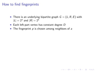
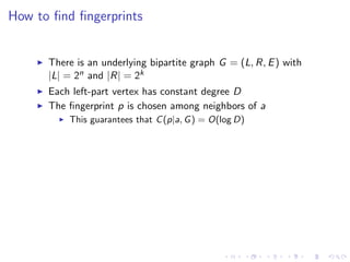
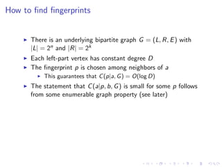
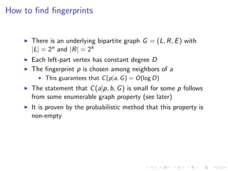
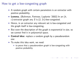
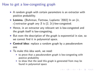
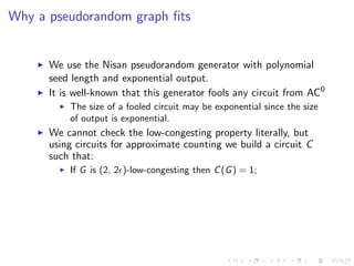
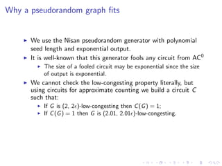
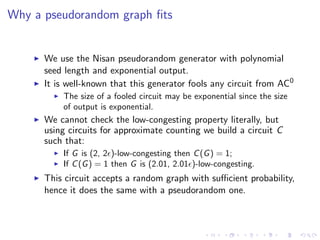
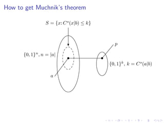
The document discusses improvements to the space-bounded version of Muchnik's conditional complexity theorem through 'naive' derandomization. It introduces concepts such as Kolmogorov complexity and demonstrates a method to transform random graphs into pseudorandom ones to enhance performance in polynomial space. The key focus is on obtaining low-congesting graphs and showing their properties via pseudorandom generators.

1. Improving the Space-Bounded Version of
Muchnik’s Conditional Complexity Theorem via
“Naive” Derandomization
Daniil Musatov1
1 Lomonosov Moscow State University,
St. Petersburg, June 14th, 2011

2. Some disclaimers
This talk is in some sense a continuation of the previous one

3. Some disclaimers
This talk is in some sense a continuation of the previous one
A similar technique is used to obtain a different result

4. Some disclaimers
This talk is in some sense a continuation of the previous one
A similar technique is used to obtain a different result
Why “naive”?

5. Some disclaimers
This talk is in some sense a continuation of the previous one
A similar technique is used to obtain a different result
Why “naive”? Because we simply replace a random object by
a pseudo-random one and it still does the job.

6. Kolmogorov complexity
Kolmogorov complexity C (a|b) of a string a conditional to b
is the minimal length of a program p that produces a given b,
i.e., p(b) = a

7. Kolmogorov complexity
Kolmogorov complexity C (a|b) of a string a conditional to b
is the minimal length of a program p that produces a given b,
i.e., p(b) = a
Space-bounded version: C s (a|b) is the minimal length of a
program p such that p(b) = a

8. Kolmogorov complexity
Kolmogorov complexity C (a|b) of a string a conditional to b
is the minimal length of a program p that produces a given b,
i.e., p(b) = a
Space-bounded version: C s (a|b) is the minimal length of a
program p such that p(b) = a and the computation of p(b)
performs in space s.

9. Muchnik’s theorem
Muchnik’s theorem (TCS’2002): For any a and b of length n
there exists p of length C (a|b) + O(log n) such that p(b) = a

10. Muchnik’s theorem
Muchnik’s theorem (TCS’2002): For any a and b of length n
there exists p of length C (a|b) + O(log n) such that p(b) = a
and C (p|a) = O(log n).

11. Muchnik’s theorem
Muchnik’s theorem (TCS’2002): For any a and b of length n
there exists p of length C (a|b) + O(log n) such that p(b) = a
and C (p|a) = O(log n).
Space-bounded version (M., Romashchenko, Shen, CSR’2009,
ToCS’2011): For any a and b of length n and for any s there
exists p of length C s (a|b) + O(log3 n) such that:

12. Muchnik’s theorem
Muchnik’s theorem (TCS’2002): For any a and b of length n
there exists p of length C (a|b) + O(log n) such that p(b) = a
and C (p|a) = O(log n).
Space-bounded version (M., Romashchenko, Shen, CSR’2009,
ToCS’2011): For any a and b of length n and for any s there
exists p of length C s (a|b) + O(log3 n) such that:
p(b) = a;
the computation of p(b) performs in space O(s) + poly(n)
and C poly(n) (p|a) = O(log3 n)

13. Muchnik’s theorem
Muchnik’s theorem (TCS’2002): For any a and b of length n
there exists p of length C (a|b) + O(log n) such that p(b) = a
and C (p|a) = O(log n).
Space-bounded version (M., Romashchenko, Shen, CSR’2009,
ToCS’2011): For any a and b of length n and for any s there
exists p of length C s (a|b) + O(log3 n) such that:
p(b) = a;
the computation of p(b) performs in space O(s) + poly(n)
and C poly(n) (p|a) = O(log3 n)
In current work we get rid of polylogarithmic terms and make
them again logarithmic

14. Proof of Muchnik’s theorem: fingerprints
{0, 1}n , n = |a|
{0, 1}k , k = C(a|b)
a

15. Proof of Muchnik’s theorem: fingerprints
p
{0, 1}n , n = |a|
{0, 1}k , k = C(a|b)
a
p is a fingerprint of a

16. Proof of Muchnik’s theorem: fingerprints
p
{0, 1}n , n = |a|
{0, 1}k , k = C(a|b)
a
p is a fingerprint of a
For C (p|a) to be small, there should be few fingerprints for each a

17. Proof of Muchnik’s theorem: fingerprints
S = {x: C(x|b) ≤ C(a|b)}
p
{0, 1}n , n = |a|
{0, 1}k , k = C(a|b)
a
p is a fingerprint of a
For C (p|a) to be small, there should be few fingerprints for each a
For C (a|p, b) to be small,

18. Proof of Muchnik’s theorem: fingerprints
S = {x: C(x|b) ≤ C(a|b)}
p
{0, 1}n , n = |a|
{0, 1}k , k = C(a|b)
a
p is a fingerprint of a
For C (p|a) to be small, there should be few fingerprints for each a
For C (a|p, b) to be small, there should be few preimages of p in S

19. How to find fingerprints
There is an underlying bipartite graph G = (L, R, E ) with
|L| = 2n and |R| = 2k

20. How to find fingerprints
There is an underlying bipartite graph G = (L, R, E ) with
|L| = 2n and |R| = 2k
Each left-part vertex has constant degree D

21. How to find fingerprints
There is an underlying bipartite graph G = (L, R, E ) with
|L| = 2n and |R| = 2k
Each left-part vertex has constant degree D
The fingerprint p is chosen among neighbors of a

22. How to find fingerprints
There is an underlying bipartite graph G = (L, R, E ) with
|L| = 2n and |R| = 2k
Each left-part vertex has constant degree D
The fingerprint p is chosen among neighbors of a
This guarantees that C (p|a, G ) = O(log D)

23. How to find fingerprints
There is an underlying bipartite graph G = (L, R, E ) with
|L| = 2n and |R| = 2k
Each left-part vertex has constant degree D
The fingerprint p is chosen among neighbors of a
This guarantees that C (p|a, G ) = O(log D)
The statement that C (a|p, b, G ) is small for some p follows
from some enumerable graph property (see later)

24. How to find fingerprints
There is an underlying bipartite graph G = (L, R, E ) with
|L| = 2n and |R| = 2k
Each left-part vertex has constant degree D
The fingerprint p is chosen among neighbors of a
This guarantees that C (p|a, G ) = O(log D)
The statement that C (a|p, b, G ) is small for some p follows
from some enumerable graph property (see later)
It is proven by the probabilistic method that this property is
non-empty

25. How to find fingerprints
There is an underlying bipartite graph G = (L, R, E ) with
|L| = 2n and |R| = 2k
Each left-part vertex has constant degree D
The fingerprint p is chosen among neighbors of a
This guarantees that C (p|a, G ) = O(log D)
The statement that C (a|p, b, G ) is small for some p follows
from some enumerable graph property (see later)
It is proven by the probabilistic method that this property is
non-empty
Hence, the first graph in the enumeration has small complexity

26. How to find fingerprints
There is an underlying bipartite graph G = (L, R, E ) with
|L| = 2n and |R| = 2k
Each left-part vertex has constant degree D
The fingerprint p is chosen among neighbors of a
This guarantees that C (p|a, G ) = O(log D)
The statement that C (a|p, b, G ) is small for some p follows
from some enumerable graph property (see later)
It is proven by the probabilistic method that this property is
non-empty
Hence, the first graph in the enumeration has small complexity
Hence, C (p|a) and C (a|p, b) are also small

27. What graph properties do we need?
Some graph properties leading to Muchnik’s theorem:
(Muchnik) Expander-like property

28. What graph properties do we need?
Some graph properties leading to Muchnik’s theorem:
(Muchnik) Expander-like property
(MRS) Possibility of online matching

29. What graph properties do we need?
Some graph properties leading to Muchnik’s theorem:
(Muchnik) Expander-like property
(MRS) Possibility of online matching
(MRS) Extractor

30. What graph properties do we need?
Some graph properties leading to Muchnik’s theorem:
(Muchnik) Expander-like property
(MRS) Possibility of online matching
(MRS) Extractor
(This paper) “Low-congesting”

31. The essential property: low-congesting graph
S, |S| < 2k
{0, 1}n
each vertex has D neighbors
{0, 1}k

32. The essential property: low-congesting graph
S, |S| < 2k
α-clot
{0, 1}
n
each vertex has D neighbors
{0, 1}k
α-clot for S is the set of all vertices having more than αD
neighbors in S.

33. The essential property: low-congesting graph
S, |S| < 2k
α-clot
{0, 1}
n
each vertex has D neighbors
{0, 1}k
α-congested vertex
α-clot for S is the set of all vertices having more than αD
neighbors in S.
A vertex is α-congested if all its neighbors lie in α-clot.

34. The essential property: low-congesting graph
S, |S| < 2k
α-clot
{0, 1}
n
each vertex has D neighbors
{0, 1}k
α-congested vertex
α-clot for S is the set of all vertices having more than αD
neighbors in S.
A vertex is α-congested if all its neighbors lie in α-clot.
The set S is (α, β)-low-congested if it contains less than βK
α-congested vertices.

35. The essential property: low-congesting graph
α-clot for S is the set of all vertices having more than αD
neighbors in S.
A vertex is α-congested if all its neighbors lie in α-clot.
The set S is (α, β)-low-congested if it contains less than βK
α-congested vertices.
We call a set relevant if it has the form {x|C s (x|b) < k}.
We call a graph (α, β)-low-congesting if all relevant sets are
(α, β)-low-congested.

36. How to get a low-congesting graph
A random graph with certain parameters is an extractor with
positive probability.

37. How to get a low-congesting graph
A random graph with certain parameters is an extractor with
positive probability.
Lemma. (Buhrman, Fortnow, Laplante ’2002) In an (k,
)-extractor graph any S is (2, 2 )-low-congested.
Hence, in an extractor any relevant set is low-congested and
the graph itself is low-congesting.

38. How to get a low-congesting graph
A random graph with certain parameters is an extractor with
positive probability.
Lemma. (Buhrman, Fortnow, Laplante ’2002) In an (k,
)-extractor graph any S is (2, 2 )-low-congested.
Hence, in an extractor any relevant set is low-congested and
the graph itself is low-congesting.
But even the description of the graph is exponential in size, so
we cannot find it in polynomial space.

39. How to get a low-congesting graph
A random graph with certain parameters is an extractor with
positive probability.
Lemma. (Buhrman, Fortnow, Laplante ’2002) In an (k,
)-extractor graph any S is (2, 2 )-low-congested.
Hence, in an extractor any relevant set is low-congested and
the graph itself is low-congesting.
But even the description of the graph is exponential in size, so
we cannot find it in polynomial space.
Central idea: replace a random graph by a pseudorandom
one
To make this idea work, we need:

40. How to get a low-congesting graph
A random graph with certain parameters is an extractor with
positive probability.
Lemma. (Buhrman, Fortnow, Laplante ’2002) In an (k,
)-extractor graph any S is (2, 2 )-low-congested.
Hence, in an extractor any relevant set is low-congested and
the graph itself is low-congesting.
But even the description of the graph is exponential in size, so
we cannot find it in polynomial space.
Central idea: replace a random graph by a pseudorandom
one
To make this idea work, we need:
to prove that a pseudorandom graph is low-congesting with
positive probability

41. How to get a low-congesting graph
A random graph with certain parameters is an extractor with
positive probability.
Lemma. (Buhrman, Fortnow, Laplante ’2002) In an (k,
)-extractor graph any S is (2, 2 )-low-congested.
Hence, in an extractor any relevant set is low-congested and
the graph itself is low-congesting.
But even the description of the graph is exponential in size, so
we cannot find it in polynomial space.
Central idea: replace a random graph by a pseudorandom
one
To make this idea work, we need:
to prove that a pseudorandom graph is low-congesting with
positive probability
to show that the seed this graph is generated from may be
found in polynomial space

42. Why a pseudorandom graph fits
We use the Nisan pseudorandom generator with polynomial
seed length and exponential output.

43. Why a pseudorandom graph fits
We use the Nisan pseudorandom generator with polynomial
seed length and exponential output.
It is well-known that this generator fools any circuit from AC0

44. Why a pseudorandom graph fits
We use the Nisan pseudorandom generator with polynomial
seed length and exponential output.
It is well-known that this generator fools any circuit from AC0
The size of a fooled circuit may be exponential since the size
of output is exponential.

45. Why a pseudorandom graph fits
We use the Nisan pseudorandom generator with polynomial
seed length and exponential output.
It is well-known that this generator fools any circuit from AC0
The size of a fooled circuit may be exponential since the size
of output is exponential.
We cannot check the low-congesting property literally, but
using circuits for approximate counting we build a circuit C
such that:

46. Why a pseudorandom graph fits
We use the Nisan pseudorandom generator with polynomial
seed length and exponential output.
It is well-known that this generator fools any circuit from AC0
The size of a fooled circuit may be exponential since the size
of output is exponential.
We cannot check the low-congesting property literally, but
using circuits for approximate counting we build a circuit C
such that:
If G is (2, 2 )-low-congesting then C (G ) = 1;

47. Why a pseudorandom graph fits
We use the Nisan pseudorandom generator with polynomial
seed length and exponential output.
It is well-known that this generator fools any circuit from AC0
The size of a fooled circuit may be exponential since the size
of output is exponential.
We cannot check the low-congesting property literally, but
using circuits for approximate counting we build a circuit C
such that:
If G is (2, 2 )-low-congesting then C (G ) = 1;
If C (G ) = 1 then G is (2.01, 2.01 )-low-congesting.

48. Why a pseudorandom graph fits
We use the Nisan pseudorandom generator with polynomial
seed length and exponential output.
It is well-known that this generator fools any circuit from AC0
The size of a fooled circuit may be exponential since the size
of output is exponential.
We cannot check the low-congesting property literally, but
using circuits for approximate counting we build a circuit C
such that:
If G is (2, 2 )-low-congesting then C (G ) = 1;
If C (G ) = 1 then G is (2.01, 2.01 )-low-congesting.
This circuit accepts a random graph with sufficient probability,
hence it does the same with a pseudorandom one.

49. The circuit
S
h1 (x1 ) h2 (x1 ) ··· hD (x1 ) h1 (x2 ) ··· hD (x2 ) ···
≡ ··· ≡ ≡ ··· ≡ ··· ≡ ···
Counting circuit Counting circuit
1, if Σinputs > 2.01D 1, if Σinputs > 2.01D ···
0, if Σinputs < 2D 0, if Σinputs < 2D
∧ ···
Counting circuit
1, if Σinputs < 2ϵK
0, if Σinputs > 2.01ϵK
∧S

50. How to get Muchnik’s theorem
Firstly, we search for a good seed for the generator and fix it.
This search needs only polynomial space.

51. How to get Muchnik’s theorem
Firstly, we search for a good seed for the generator and fix it.
This search needs only polynomial space.
If a is not congested in {x|C s (x|b) < k} then it has a
neighbor p outside the clot.
This p satisfies all requirements.

52. How to get Muchnik’s theorem
S = {x: C s (x|b) ≤ k}
p
{0, 1}n , n = |a|
{0, 1}k , k = C s (a|b)
a

53. How to get Muchnik’s theorem
Firstly, we search for a good seed for the generator and fix it.
This search needs only polynomial space.
If a is not congested in {x|C s (x|b) < k} then it has a
neighbor p outside the clot.
This p satisfies all requirements.
If a is congested then we repeat the whole construction
replacing the relevant sets by the sets of congested vertices in
relevant sets.

54. How to get Muchnik’s theorem
Firstly, we search for a good seed for the generator and fix it.
This search needs only polynomial space.
If a is not congested in {x|C s (x|b) < k} then it has a
neighbor p outside the clot.
This p satisfies all requirements.
If a is congested then we repeat the whole construction
replacing the relevant sets by the sets of congested vertices in
relevant sets.
There may be several iterations but since the upper bound on
the size of a relevant set decreases exponentially there is at
most linear number of steps, hence all polynomial bounds
remain.

55. The final formulation
For any a and b of length n and for any s there exists p of length
C s (a|b) + O(log log s + log n) such that:
p(b) = a;
the computation of p(b) performs in space O(s) + poly(n)
and C O(s)+poly(n) (p|a) = O(log log s + log n)

56. Summary of the technology
Take some theorem about Kolmogorov complexity relying on
the existence of some combinatorial object

57. Summary of the technology
Take some theorem about Kolmogorov complexity relying on
the existence of some combinatorial object
Build a constant-depth circuit recognizing this object

58. Summary of the technology
Take some theorem about Kolmogorov complexity relying on
the existence of some combinatorial object
Build a constant-depth circuit recognizing this object
Replace a random object by a pseudorandom one

59. Summary of the technology
Take some theorem about Kolmogorov complexity relying on
the existence of some combinatorial object
Build a constant-depth circuit recognizing this object
Replace a random object by a pseudorandom one
Obtain a space-bounded version of the theorem

60. Summary of the technology
Take some theorem about Kolmogorov complexity relying on
the existence of some combinatorial object
Build a constant-depth circuit recognizing this object
Replace a random object by a pseudorandom one
Obtain a space-bounded version of the theorem
???????
PROFIT

61. Thank you!
mailto:musatych@gmail.com
http://musatych.livejournal.com