Download as PDF, PPTX

![Motivations
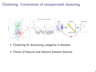
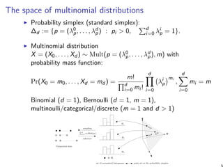
Which geometry and distance are appropriate for a space of
probability distributions? for a space of correlation matrices?
Information geometry [5] focuses on the differential-geometric
structures associated to spaces of parametric distributions...
Benchmark different geometric space modelings
3](https://image.slidesharecdn.com/slides-clusteringhilbertgeometryml-181212073307/85/Clustering-in-Hilbert-geometry-for-machine-learning-3-320.jpg)


![The shape of ℓ1-balls in ∆d
For trinomials in ∆2 (with λ2 = 1 − (λ0 + λ1)), the ρL1
distance is given by:
ρL1(p, q) = |λ0
p − λ0
q| + |λ1
p − λ1
q| + |λ0
q − λ0
p + λ1
q − λ1
p|.
ℓ1-distance is polytopal: cross-polytope
Z = conv(±ei : i ∈ [d]) also called co-cube (orthoplex)
Shape of ℓ1-balls:
BallL1 (p, r) = (λp ⊕ rZ) ∩ H∆d
In 2D, regular octahedron cut by H∆2 = hexagonal shapes.
9](https://image.slidesharecdn.com/slides-clusteringhilbertgeometryml-181212073307/85/Clustering-in-Hilbert-geometry-for-machine-learning-9-320.jpg)
![Visualizing the 1D/2D/3D shapes of L1 balls in ∆d
Illustration courtesy of ’Geometry of Quantum States’, [1]
10](https://image.slidesharecdn.com/slides-clusteringhilbertgeometryml-181212073307/85/Clustering-in-Hilbert-geometry-for-machine-learning-10-320.jpg)
![Fisher-Hotelling-Rao Riemannian geometry (1930)
Fisher metric tensor [gij] (constant positive curvature):
gij(p) =
δij
λi
p
+
1
λ0
p
.
Statistical invariance yields unique Fisher metric [2]
Distance is a geodesic length (Levi-Civita connection ∇LC
with metric-compatible parallel transport)
Rao metric distance between two multinomials on Riemannian
manifold (∆d , g):
ρFHR(p, q) = 2 arccos
( d∑
i=0
√
λi
pλi
q
)
.
Can be embedded in the positive orthant of an Euclidean
d-sphere of Rd+1 by using the square root representation
λ →
√
λ = (
√
λ0, . . . ,
√
λd )
11](https://image.slidesharecdn.com/slides-clusteringhilbertgeometryml-181212073307/85/Clustering-in-Hilbert-geometry-for-machine-learning-11-320.jpg)

![Euclidean shape of balls in Hilbert projective geometry
Hilbert balls in ∆d : hexagons shapes (2D) [10], rhombic
dodecahedra (3D), polytopes [4] with d(d + 1) facets in
dimension d.
1.5
3.0
4.5
6.0
Not Riemannian/differential-geometric geometry because
infinitesimally small balls have not ellipsoidal shapes. (Tissot
indicatrix in Riemannian geometry)
A video explaining the shapes of Hilbert balls:
https://www.youtube.com/watch?v=XE5x5rAK8Hk&t=1s
14](https://image.slidesharecdn.com/slides-clusteringhilbertgeometryml-181212073307/85/Clustering-in-Hilbert-geometry-for-machine-learning-14-320.jpg)
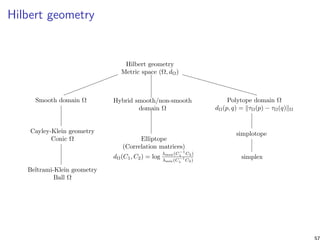
![Hilbert geometry generalizes Cayley-Klein hyperbolic
geometry
Defined for a quadric domain
(curved elliptical/hyperbolic Mahalanobis distances [6])
Video: https://www.youtube.com/watch?v=YHJLq3-RL58
17](https://image.slidesharecdn.com/slides-clusteringhilbertgeometryml-181212073307/85/Clustering-in-Hilbert-geometry-for-machine-learning-17-320.jpg)
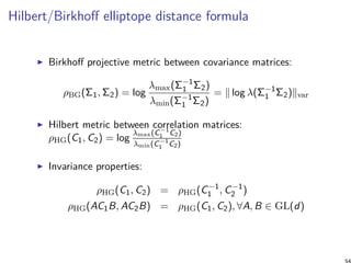
![Relationship with Birkhoff projective geometry
Instead of considering the (d − 1)-dimensional simplex ∆d ,
consider the the pointed cone Rd
+,∗.
Birkhoff projective metric on positive histograms:
ρBG(˜p, ˜q) := log maxi,j∈[d]
˜pi ˜qj
˜pj ˜qi
is scale-invariant ρBG(α˜p, β˜q) = ρBG(˜p, ˜q), for any α, β > 0.
O
˜p
˜q
p
q
e1 = (1, 0)
e2 = (0, 1)
∆1
R2
+,∗
ρHG(p, q)
ρBG(˜p, ˜q)
19](https://image.slidesharecdn.com/slides-clusteringhilbertgeometryml-181212073307/85/Clustering-in-Hilbert-geometry-for-machine-learning-19-320.jpg)
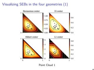
![Shape of Hilbert balls in an open simplex
A ball in the Hilbert simplex geometry has a Euclidean
polytope shape with d(d + 1) facets [4]
In 2D, Hilbert balls have 2(2 + 1) = 6 hexagonal shapes
varying with center locations. In 3D, the shape of balls are
rhombic-dodecahedron
When the domain is not simplicial, Hilbert balls can have
varying complexities [10]
No metric tensor in Hilbert geometry because infinitesimally
the ball shapes are polytopes and not ellipsoids.
Hilbert geometry can be studied via Finsler geometry
21](https://image.slidesharecdn.com/slides-clusteringhilbertgeometryml-181212073307/85/Clustering-in-Hilbert-geometry-for-machine-learning-21-320.jpg)


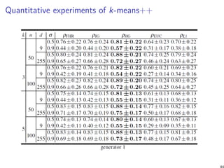
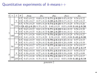
![k-means++ clustering (seeding initialization)
For an arbitrary distance D, define the k-means objective
function (NP-hard to minimize):
ED(Λ, C) =
1
n
n∑
i=1
minj∈{1,...,k}D(pi : cj)
k-means++: Pick uniformly at random at first seed c1, and
then iteratively choose the (k − 1) remaining seeds according
to the following probability distribution:
Pr(cj = pi ) =
D(pi , {c1, . . . , cj−1})
∑n
i=1 D(pi , {c1, . . . , cj−1})
(2 ≤ j ≤ k).
A randomized seeding initialization of k-means, can be further
locally optimized using Lloyd’s batch iterative updates, or
Hartigan’s single-point swap heuristic [9], etc.
28](https://image.slidesharecdn.com/slides-clusteringhilbertgeometryml-181212073307/85/Clustering-in-Hilbert-geometry-for-machine-learning-28-320.jpg)
![Performance analysis of k-means++ [8]
Let κ1 and κ2 be two constants such that κ1 defines the
quasi-triangular inequality property:
D(x : z) ≤ κ1 (D(x : y) + D(y : z)) , ∀x, y, z ∈ ∆d
,
and κ2 handles the symmetry inequality:
D(x : y) ≤ κ2D(y : x), ∀x, y ∈ ∆d
.
Theorem
The generalized k-means++ seeding guarantees with high
probability a configuration C of cluster centers such that:
ED(Λ, C) ≤ 2κ2
1(1 + κ2)(2 + log k)E∗
D(Λ, k)
29](https://image.slidesharecdn.com/slides-clusteringhilbertgeometryml-181212073307/85/Clustering-in-Hilbert-geometry-for-machine-learning-29-320.jpg)

![Performance analysis of k-means++
In any normed space (X, ∥ · ∥), the k-means++ with
D(x, y) = ∥x − y∥2 is 16(2 + log k)-competitive.
In any inner product space (X, ⟨·, ·⟩), the k-means++ with
D(x, y) = ⟨x − y, x − y⟩ is 16(2 + log k)-competitive.
Hilbert simplex geometry is isometric to a normed vector
space [4] (Theorem 3.3):
(∆d
, ρHG) ≃ (V d
, ∥ · ∥NH)
Theorem
k-means++ seeding in a Hilbert simplex geometry in fixed
dimension is 16(2 + log k)-competitive.
31](https://image.slidesharecdn.com/slides-clusteringhilbertgeometryml-181212073307/85/Clustering-in-Hilbert-geometry-for-machine-learning-31-320.jpg)


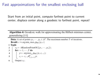
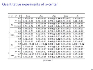
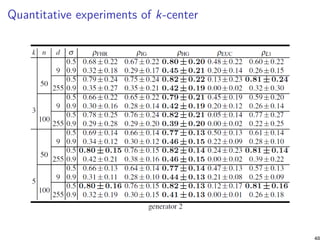
![k-Center clustering: farthest first traversal heuristic
Guaranteed approximation factor of 2 in any metric space [3]
34](https://image.slidesharecdn.com/slides-clusteringhilbertgeometryml-181212073307/85/Clustering-in-Hilbert-geometry-for-machine-learning-34-320.jpg)
![Smallest Enclosing Ball (SEB)
Given a finite point set {p1, . . . , pn} ∈ ∆d , the SEB in Hilbert
simplex geometry is centered at
c∗
= arg min
c∈∆d
maxi∈{1,...,n}ρHG(c, xi ),
with radius
r∗
= minc∈∆d maxi∈{1,...,n}ρHG(c, xi ).
Decision problem can be solved by Linear Programming (LP),
and optimization as a LP-type problem [7]
Do not scale well in high dimensions
35](https://image.slidesharecdn.com/slides-clusteringhilbertgeometryml-181212073307/85/Clustering-in-Hilbert-geometry-for-machine-learning-35-320.jpg)


![Summary and conclusion [11]
Introduced Hilbert/Birkhoff geometry for the probability
simplex (= space of categorical distributions) and the
elliptope (= space of correlation matrices). But also
simplotope (product of simplices), etc.
Hilbert simplex geometry is isometric to a normed vector
space (hilds for any Hilbert polytopal geometry)
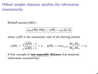
Non-separable distance that satisfies the information
monotonicity (contraction ratio of linear operator)
Novel closed form Hilbert/Birkhoff distance formula for the
correlation (metric) and covariance matrices (projective
metric)
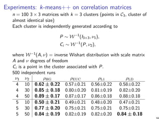
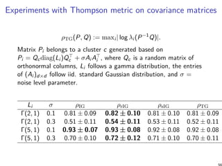
Benchmark experimentally four types of geometry for k-means
and k-center clusterings
Hilbert/Birkhoff geometry experimentally well-suited for
58](https://image.slidesharecdn.com/slides-clusteringhilbertgeometryml-181212073307/85/Clustering-in-Hilbert-geometry-for-machine-learning-58-320.jpg)
![References I
Ingemar Bengtsson and Karol Życzkowski.
Geometry of quantum states: an introduction to quantum entanglement.
Cambridge university press, 2017.
L. L. Campbell.
An extended čencov characterization of the information metric.
American Mathematical Society, 98(1):135–141, 1986.
Teofilo F Gonzalez.
Clustering to minimize the maximum intercluster distance.
Theoretical Computer Science, 38:293–306, 1985.
Bas Lemmens and Roger Nussbaum.
Birkhoff’s version of Hilbert’s metric and its applications in analysis.
Handbook of Hilbert Geometry, pages 275–303, 2014.
Frank Nielsen.
An elementary introduction to information geometry.
ArXiv e-prints, August 2018.
Frank Nielsen, Boris Muzellec, and Richard Nock.
Classification with mixtures of curved Mahalanobis metrics.
In IEEE International Conference on Image Processing (ICIP), pages 241–245, 2016.
Frank Nielsen and Richard Nock.
On the smallest enclosing information disk.
Information Processing Letters, 105(3):93–97, 2008.
Frank Nielsen and Richard Nock.
Total Jensen divergences: Definition, properties and k-means++ clustering, 2013.
arXiv:1309.7109 [cs.IT].
59](https://image.slidesharecdn.com/slides-clusteringhilbertgeometryml-181212073307/85/Clustering-in-Hilbert-geometry-for-machine-learning-59-320.jpg)

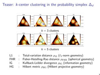
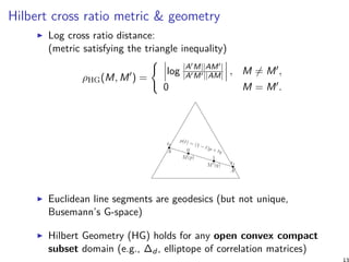
- The document discusses different geometric approaches for clustering multinomial distributions, including total variation distance, Fisher-Rao distance, Kullback-Leibler divergence, and Hilbert cross-ratio metric. - It benchmarks k-means clustering using these four geometries on the probability simplex, finding that Hilbert geometry clustering yields good performance with theoretical guarantees. - The Hilbert cross-ratio metric defines a non-Riemannian Hilbert geometry on the simplex with polytopal balls, and satisfies information monotonicity properties desirable for clustering distributions.