This document discusses temporal graphs, which are graphs where nodes and edges are active for specific time instances. It provides examples of temporal graphs and compares them to non-temporal graphs. It then covers temporal graph traversal methods like depth-first search and breadth-first search, accounting for temporal constraints. Various path types in temporal graphs are defined, such as foremost paths, latest-departure paths, and fastest paths. Algorithms for finding these paths using a stream representation or graph transformation approach are outlined.

1. Temporal Graph : Storage,
Traversal, Path discovery
Submitted by
Vinay Sarda
M.Tech(CSE) II Year
13535054
Under the guidance of
Prof. A.K. Sarje

2. Outline
 Introduction
 Graph Database
 What is a Temporal Graph
 Traversal in Temporal Path
 Types of Path in Temporal Graph
 Algorithms to determine different temporal path
 Conclusion

3. Introduction
 Graph database are best tool for handling highly connected data
 In Relational or Hierarchical database, some entities have precedence over other
like key, parent etc.
 In Graph No node or edge have a higher precedence over other
 Graph DB are NOSQL, doesn’t have rigid schema
 Graph uses structures like nodes, edges are used to store and represent data
 No need to look-up for neighbours as it provides index-free adjacency
 Graph DB can be used in to determine whether two concept are related or not, or
is it possible to reach from source to destination within specified interval etc.

4. Example -Graph
Roy is boy
Mary is a girl
Roy and Mary are friends

5. Accessing Graph DB
 TinkerPop is an open source toolkit that provides
interfaces to implement Blueprint
 Blueprint is a generic graph API, serves as a base layer for
graph DB architectures
 Pipes is a dataflow network using process graphs
 Gremlin is a graph traversal language for accessing and
manipulating graphs
 Frames allows developer to frame a graph element in
terms of java interface
 Furnace is a graph algorithm package
 Rexster is a graph server that exploits blueprint via REST
 Example Titan Graph DB
TinkerPop Stack

6. Temporal Graph
 Nodes and Edges are active for a specific time instance
 Visiting nodes or edges at any time other than specific time instance is not possible
 Example – SMS Network, flight scheduling, stock exchange network
 Did mail from A to D had any impact on mail send from D to B
Sender Receipent Time
A B 0
A C,E 1
E D 3
B C 5
B D 9
D B 14
A D 20
C A
B D E
1
C A
5 0
20
1
9
B D E
14
3
Non-Temporal Graph Temporal Graph

7. Temporal Graph Traversal
 Depth First Traversal
 Temporal Constraint – In traversal from node a to e set of edges {(a,b,1),(b,e,6)} is valid,
but edge set {(a,b,9),(b,e,6)} is not
 Multiple edges – When multiple edges occur among the same pair of nodes, only one
edge has to be chosen avoiding combinatorial effect
 Edge with highest timestamp value (most recent connection)
 Edge with lowest timestamp value (first connection)
A
B C
E
D
F
3
2
8
6
7
1
4
5
9

8. Depth First Traversal
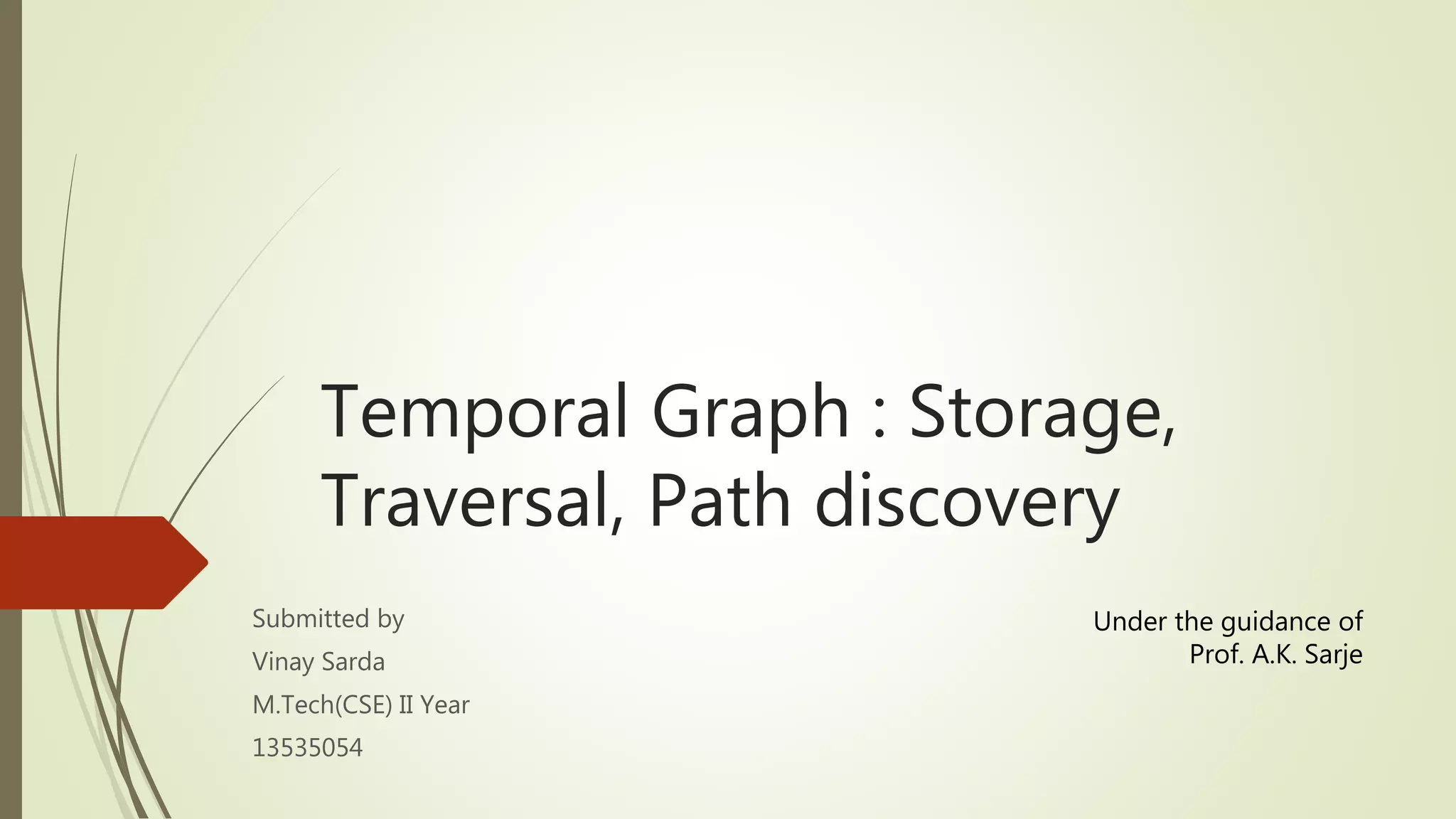
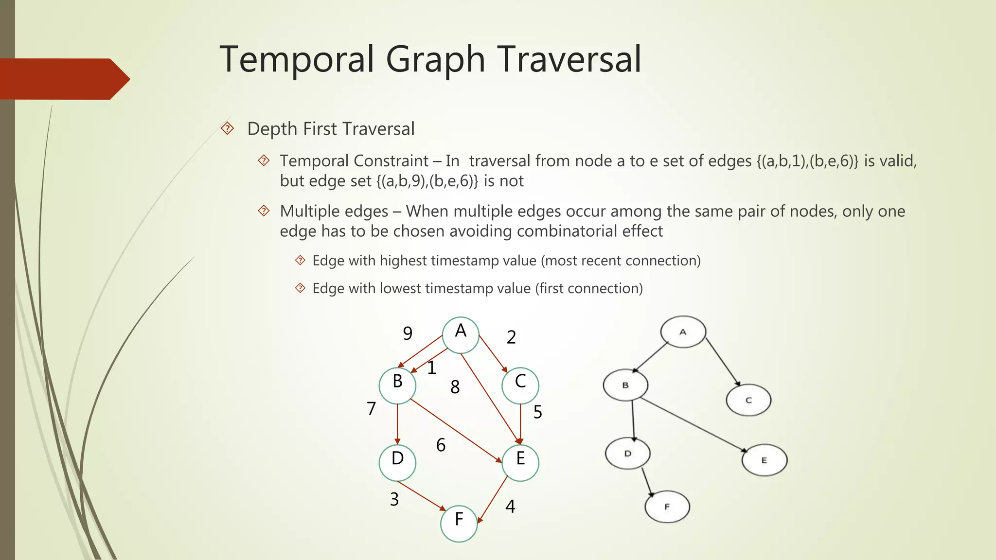
 Create a DFS tree rooted at node ‘a’ with lowest timestamp value
 Initially every node’s visiting time is infinite
 At node ‘a’, Eset = {(a,b,9), (a,b,1), (a,e,8), (a,c,2)}
 Take edge (a,b,1) and visit node ‘b’ and mark time 1
 Now Eset = {(b,d,7), (b,e,6)} and take edge (b,e,6), mark time t[e] = 6, and then (b,d,7), mark
time t[d] = 7, and so on
a
b c
e
d
2
7
1
5
a
c
e
b
d
3 f
2
8
6
7
1
4
9
5
6

9. Breadth First Traversal
 Challenges
 Temporal Constraint
 Edges (b, d, 3) and (d, e, 3) forms a valid set of consecutive edges, but (c, d, 5), (d, e, 3) doesn’t.
 Smallest path may not be earliest path
 Path from a to d takes only one hop at time t = 7, while the earliest time at which d can be reached from
a is 3 using edges (a, b, 2) and (b, d, 3)
 If we mark node ‘d’ using edge a-d and don’t consider it again then ‘e’ cannot be reached
 Multiple occurrences of a node are possible
 Terminology
 u – node
 dist(u) – distance of node u from source s
 σ(u) – earliest arrival time to reach node u from source node s
 p(u) – parent node of u
 Temporal edge is denoted as (u, v, t)
a
b c
d
e
2
5
4
7
3 5
3

10.  While Q is not empty for each node v
 If v is not in Q (whether v has been visited or not) traverse e, and if σ(v) > t, then visit v
and push (v, dist(v) = dist(u) + 1, σ (v) = t, p(v) = u) into Q.
 Else
 If there exists (v, dist(v), σ (v), p(v)) in Q such that dist(v) = dist(u) + 1: traverse e, and if σ(v) > t,
then visit v and update σ(v) = t and p(v) = u in Q
 Else (i.e., dist(v) = dist(u)): traverse e, and if σ(v) > t, then visit v and push (v, dist(v) = dist(u) + 1,
σ (v) = t, p(v) = u) into Q.
a
b c
d
e
2
5
4
7
3 5
3
c
a
b
d
e
2
4
3
d
7
3
(a, 0, 1, φ) (b, 1, 2, a) (d, 1, 7, a) (c, 1, 4, a) (d, 2, 3, b) (e, 3, 3, d)
Q (u, dist(u), σ(u), p(v))

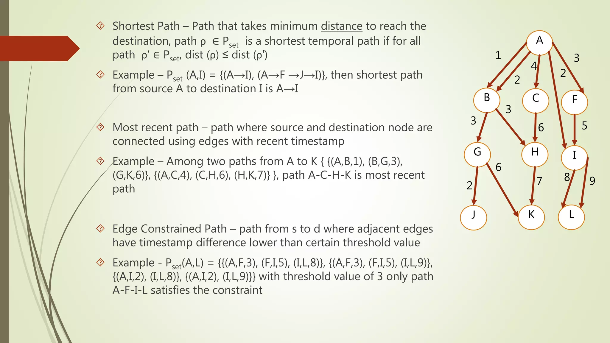
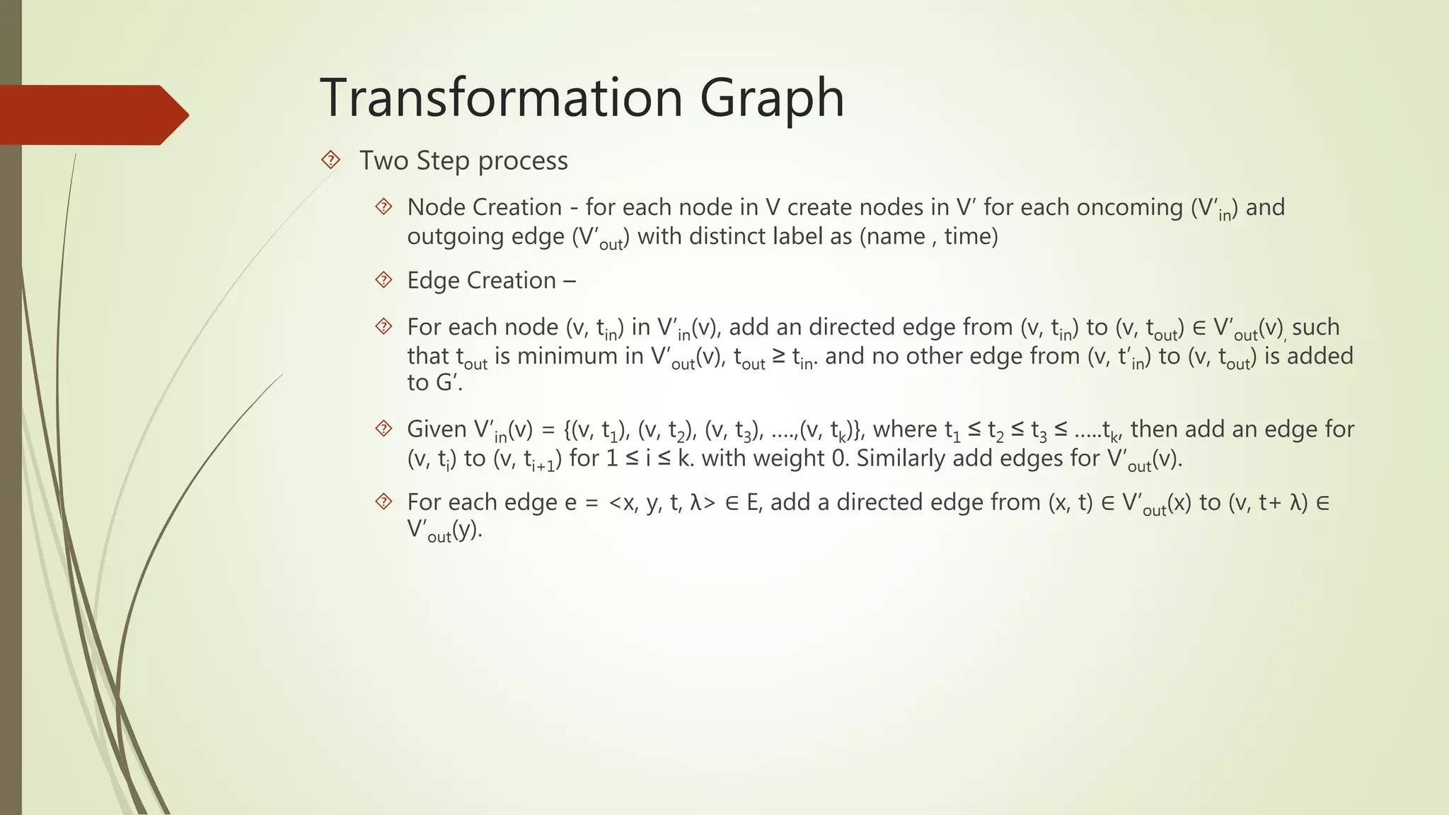
11. Paths in Temporal Graph
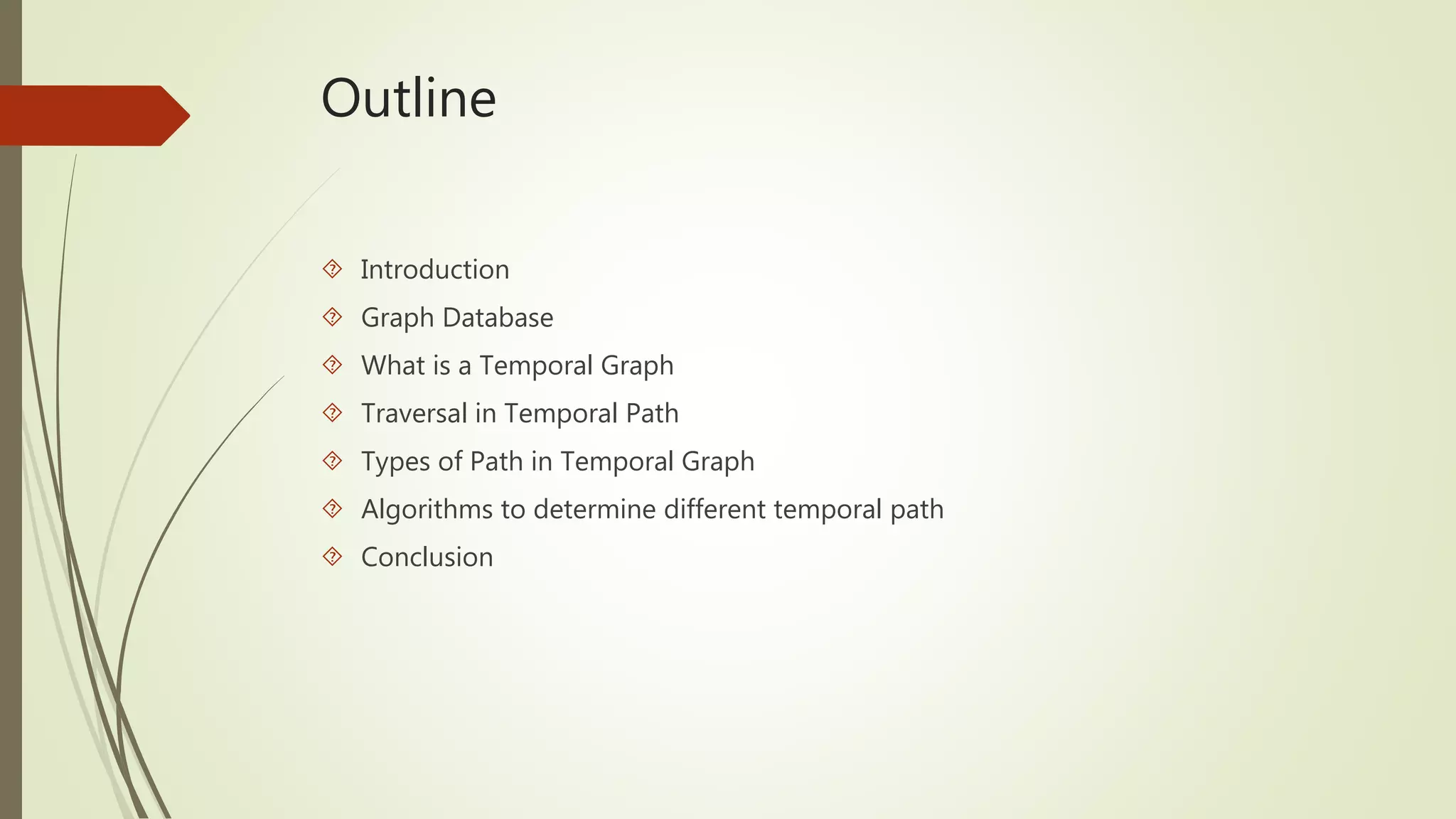
 A path ρ = {(s, u1, t1), (u1, u2, t2), (u2, u3, t3),……..,(ui-1, ui, ti), ….. (un-1 ,d, tn)} from
source s to destination d is a temporal path if ti ≤ ti+1
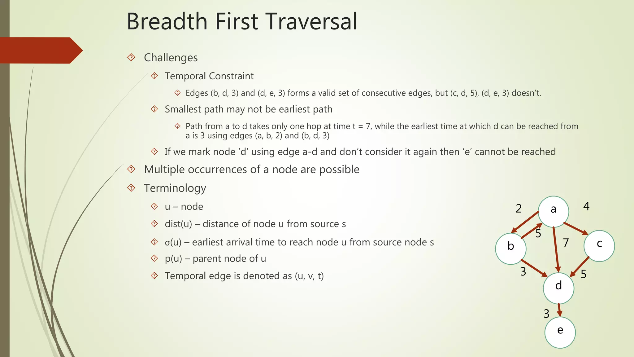
 Terminology
 Pset - set of all paths from source s to destination d
 [ta, tb] – time interval
 t[u] – time at which node u can be reached from source s
 tstart(ρ) - timestamp of a path ρ at which it starts at source s
 tend(ρ) - timestamp of a path ρ at which it ends at destination d
 dist(ρ) - number of nodes in path ρ
 duration(ρ) – time taken by path ρ to reach destination node from source node, tend(ρ) -
tstart(ρ)
 Transition time – time taken to reach from node to its neighbour node (λ), by default
assumed to be 1

12.  Foremost – In a given interval, path that reaches destination as early
as possible, path ρ ∈ Pset is a foremost path if all path ρ’ ∈ Pset, such
that tend (ρ’) ≤ tend (ρ)
 Example – Pset(A,H) = {{(A,B,1), (B,H,3)}, {(A,B,2), (B,H,3)}, {(A,C,4),
(C,H,6)}}, but only A-B-H is the foremost path
 Latest- departure path - In a given interval, path that reaches
destination as early as possible, path ρ ∈ Pset is a latest-departure
path, if all path ρ’ ∈ Pset, such that tstart (ρ’) ≤ tstart (ρ)
 Example - Pset(A,H) = {{(A,B,1), (B,H,3)}, {(A,B,2), (B,H,3)}, {(A,C,4),
(C,H,6)}}, but only A-C-H is the latest-departure path
 Fastest path – Path that spends minimum time to reach destination d
from source s, path ρ ∈ Pset is a fastest path if for all path ρ ∈ Pset,
duration (ρ) <= duration (ρ’)
 Example – Pset(B,K) = ({(B,H,3),(H,K,7)}, {(B,G,3),(G,K,6)}}, fastest path is
B-G-K as it takes only 3 units of time
A
1
2
4
2
3
B C F
3
3
6 5
G H I
6
2 7 8 9
J K L

13.  Shortest Path – Path that takes minimum distance to reach the
destination, path ρ ∈ Pset is a shortest temporal path if for all
path ρ’ ∈ Pset, dist (ρ) ≤ dist (ρ′)
 Example – Pset (A,I) = {(A→I), (A→F →J→I)}, then shortest path
from source A to destination I is A→I
 Most recent path – path where source and destination node are
connected using edges with recent timestamp
 Example – Among two paths from A to K { {(A,B,1), (B,G,3),
(G,K,6)}, {(A,C,4), (C,H,6), (H,K,7)} }, path A-C-H-K is most recent
path
 Edge Constrained Path – path from s to d where adjacent edges
have timestamp difference lower than certain threshold value
 Example - Pset(A,L) = {{(A,F,3), (F,I,5), (I,L,8)}, {(A,F,3), (F,I,5), (I,L,9)},
{(A,I,2), (I,L,8)}, {(A,I,2), (I,L,9)}} with threshold value of 3 only path
A-F-I-L satisfies the constraint
A
1
2
4
2
3
B C F
3
3
6 5
G H I
6
2 7 8 9
J K L

14. Observation
 Optimal path in Temporal Graph v/s Non-Temporal Graph
 Optimal path in Non-Temporal Graph has property that sub-path of optimal path is
always optimal
 But it doesn’t holds in case of Temporal Graph, example shortest path
A
B
C
D
2
3
7
4

15. Temporal Path Discovery Techniques
 Stream Representation of Temporal Graph
 Transformation Graph

16. Stream Representation
 Edge sequence in the order of their creation is called stream representation of
edges in a temporal graph
 Example – {(A→B)/2, (B→C)/3, (C→D)/4, (A→C)/7}
A
B
C
D
2
3
7
4

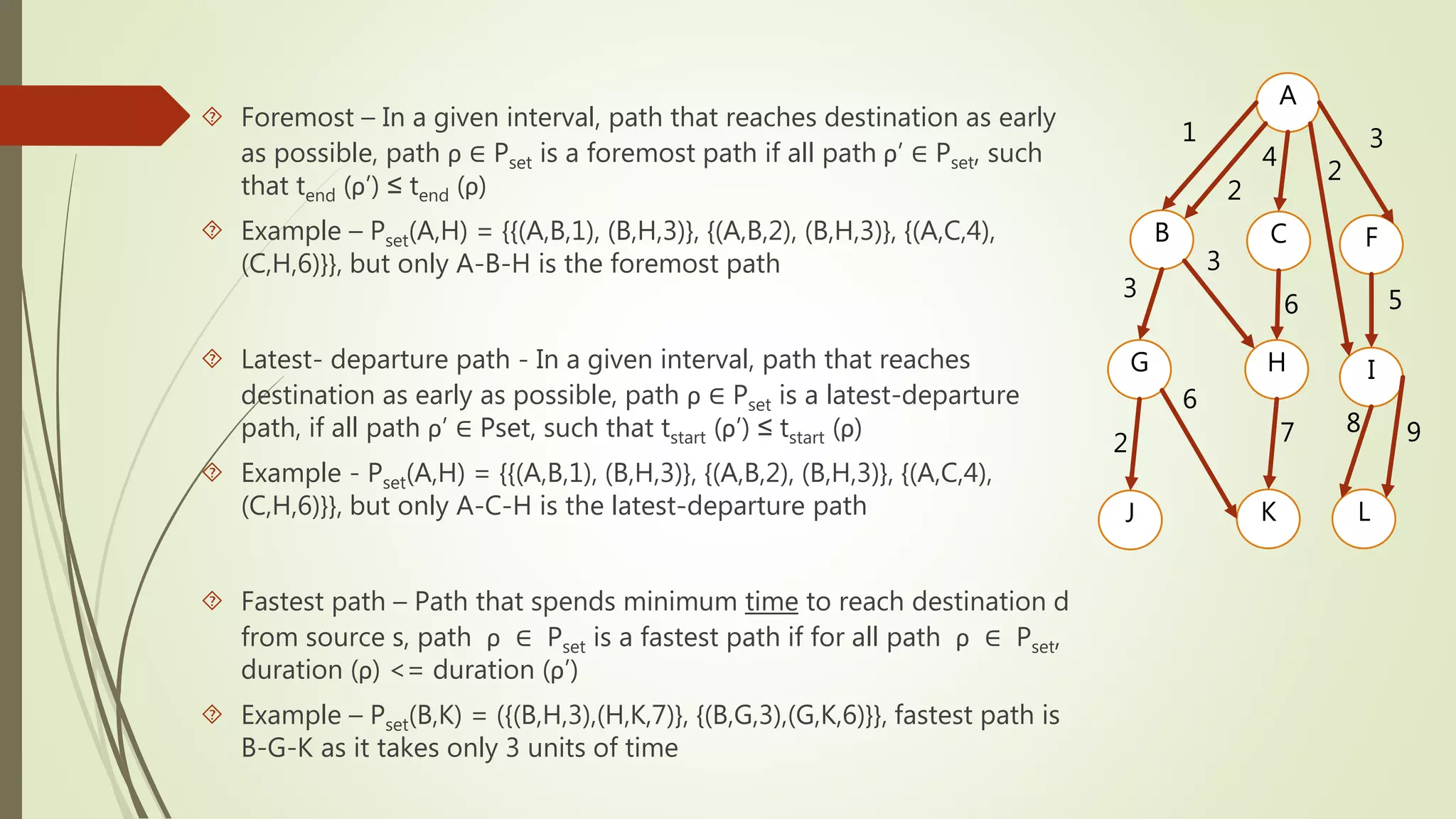
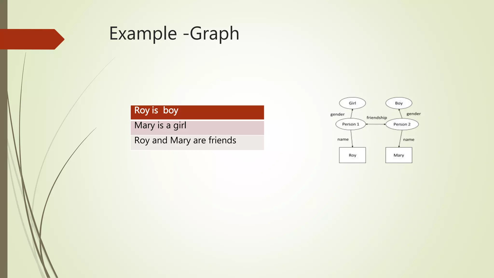
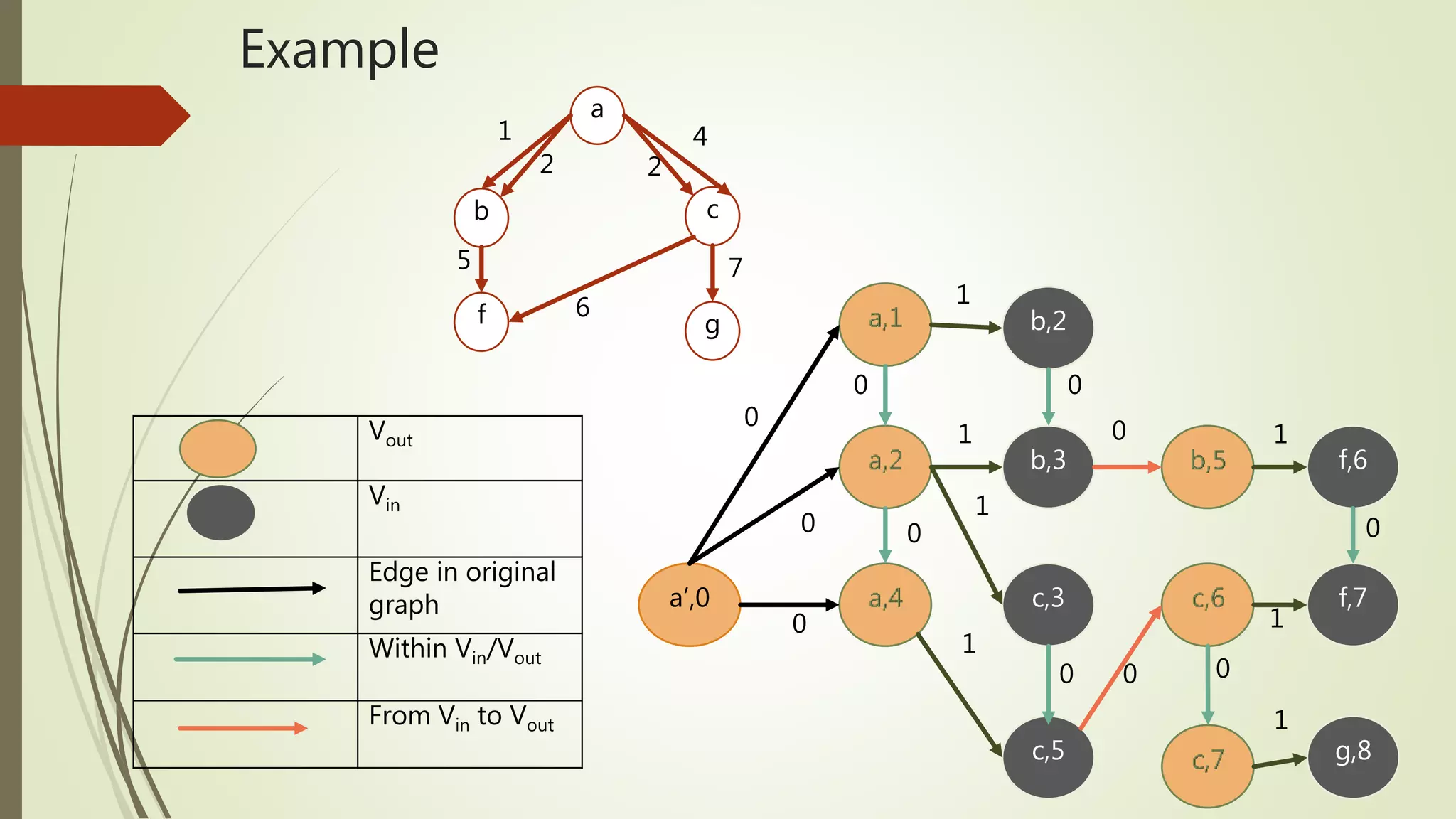
17. Foremost Path
 Foremost Path for node ‘s’ in time interval [ta,tb]
 For each node u in graph G t[u] = ∞
 Considering each edge in the sequence in the order
 Check for two conditions if true then update t[v] = t+λ
 t+λ ≤ tb and t ≥ t[u]
 t+λ < t[v]
 if t+ λ > tb then exit

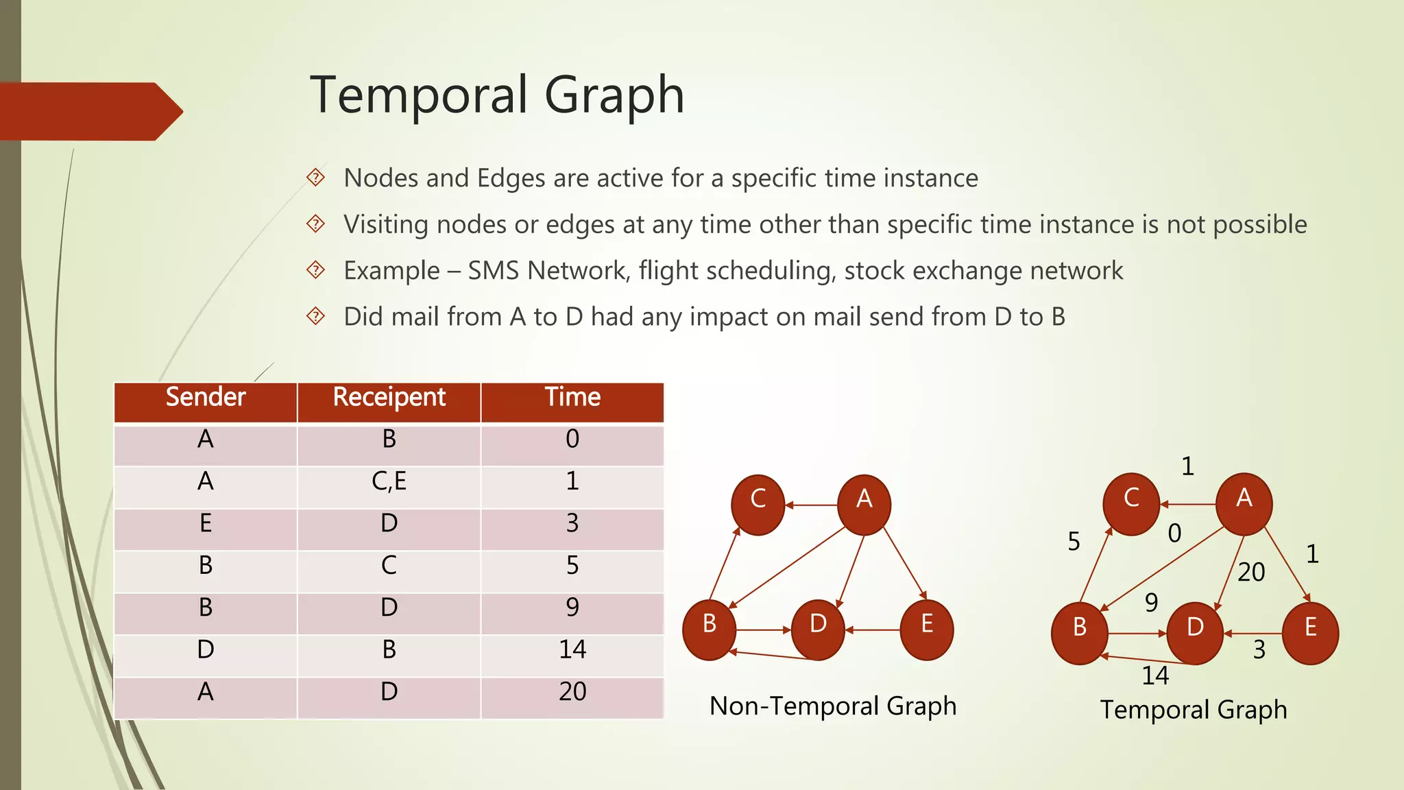
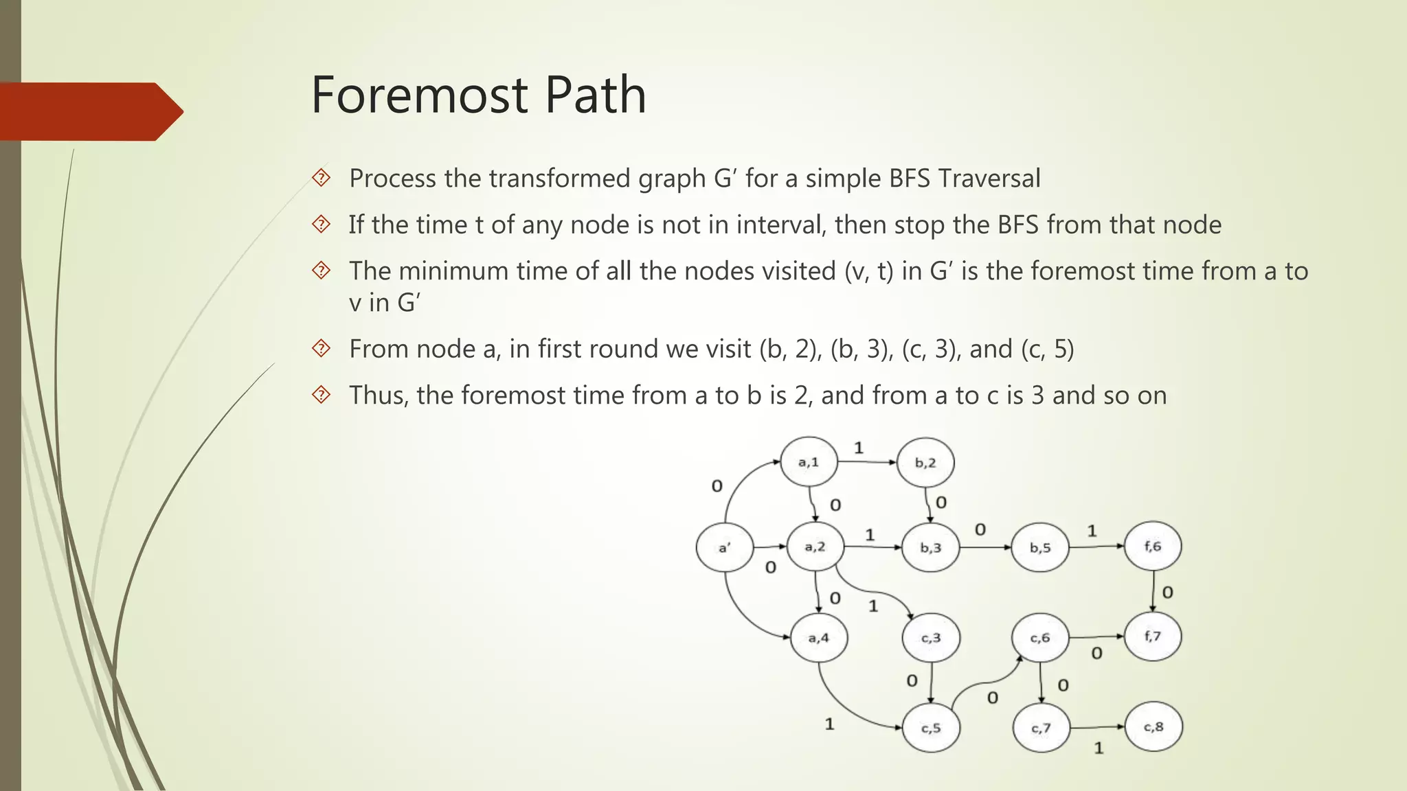
18. Example
 Edge representation is {(a, b, 1, λ), (a, c, 2, λ), (d, f, 3, λ), (b, d, 7, λ)}
 Foremost path for node ‘a’ in [1,4] assuming λ = 1
 For all node t[u] =∞
 Mark t[a] = 0
 For edge (a, b, 1, 1), t + λ = 2, satisfies conditions, update t[b] = 2
 For edge (a, c, 2, 1), t + λ = 3, satisfies conditions, update t[c] = 3
 For edge (d, f, 3, 1), t + λ = 4, doesn’t satisfies condition t ≥ t[d] as t[d] = ∞ and t =
3
t+λ ≤ tb and t ≥ t[u]
t+λ < t[v]
a
c
b
d f
3
2
7
1
∞
∞
∞
∞ ∞
0 a
3
c
b
d f
3
2
7
1
2 ∞ ∞

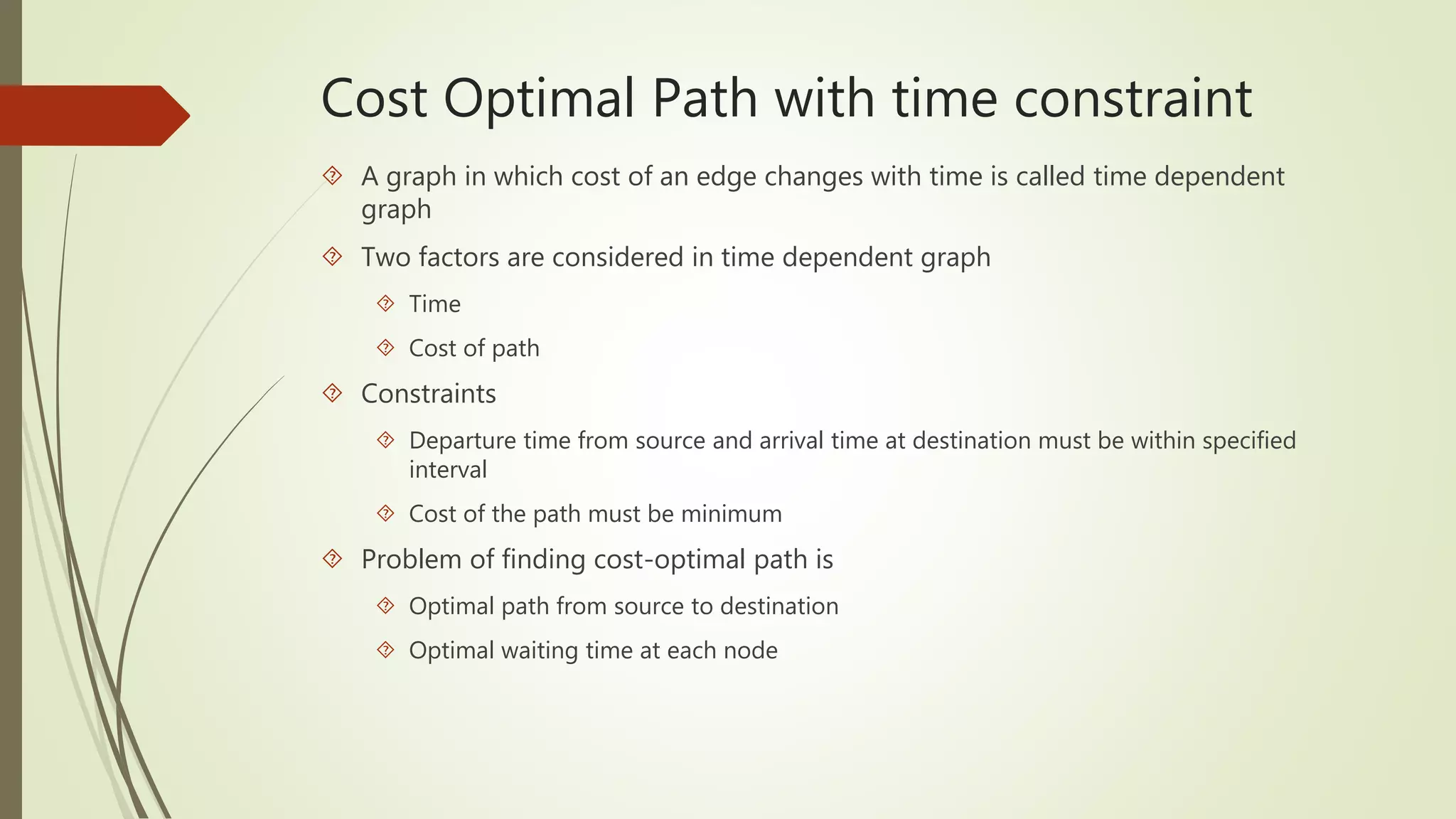
19. Fastest Path
 Lv – sorted list of foremost time for each node v from source node ‘s is maintained,
(s[v], a[v]), where s[v] represents start time from ‘s’ and a[v] arrival time at v
 If s’[v] > s[v] and a’[v] ≤ a[v], or s’[v] = s[v] and a’[v] < a[v], then (s’[v], a’[v])
dominates (s[v], a[v])
A
1
2
1,1 2,2
B D
3
5
C E
4
5
F
6
1,3
1,4
2,5
2,6
S.No. s[v] a[v]
a 1 4
b 2 4
c 4 6
d 4 5

20. Transformation Graph
 Two Step process
 Node Creation - for each node in V create nodes in V’ for each oncoming (V’in) and
outgoing edge (V’out) with distinct label as (name , time)
 Edge Creation –
 For each node (v, tin) in V’in(v), add an directed edge from (v, tin) to (v, tout) ∈ V’out(v), such
that tout is minimum in V’out(v), tout ≥ tin. and no other edge from (v, t’in) to (v, tout) is added
to G’.
 Given V’in(v) = {(v, t1), (v, t2), (v, t3), ….,(v, tk)}, where t1 ≤ t2 ≤ t3 ≤ …..tk, then add an edge for
(v, ti) to (v, ti+1) for 1 ≤ i ≤ k. with weight 0. Similarly add edges for V’out(v).
 For each edge e = <x, y, t, λ> ∈ E, add a directed edge from (x, t) ∈ V’out(x) to (v, t+ λ) ∈
V’out(y).

21. 4
a’,0
b,2
1 0 1
b,3
0 0
c,3
c,5
f,6
f,7
g,8
0
0
0
1
0 0
1
1
0 0 0
1
1
a
1
2 2
b c
f g
5
6
7
Example
Vout
Vin
Edge in original
graph
Within Vin/Vout
From Vin to Vout

22. Foremost Path
 Process the transformed graph G’ for a simple BFS Traversal
 If the time t of any node is not in interval, then stop the BFS from that node
 The minimum time of all the nodes visited (v, t) in G’ is the foremost time from a to
v in G’
 From node a, in first round we visit (b, 2), (b, 3), (c, 3), and (c, 5)
 Thus, the foremost time from a to b is 2, and from a to c is 3 and so on

23. Cost Optimal Path with time constraint
 A graph in which cost of an edge changes with time is called time dependent
graph
 Two factors are considered in time dependent graph
 Time
 Cost of path
 Constraints
 Departure time from source and arrival time at destination must be within specified
interval
 Cost of the path must be minimum
 Problem of finding cost-optimal path is
 Optimal path from source to destination
 Optimal waiting time at each node

24.  Earliest arrival time for each node is calculated so , λ1 = 0, λ2 =
10, λ3 = 15 and λ4 = 25 and time domain of g1(t), g2(t), g3(t) and
g4(t) are [0, 60], [10, 60], [15, 60] and [25, 60] respectively
 Initially ti for all node is infinite except for source s
 Priority Q is maintained containing all nodes with respect to
their ti
 In first iteration, v1 is dequeued as t1= 0 is minimum
 g2(t) and g3(t) are computed and v1 is removed from Q
 t2 = 20 and t3 = 5 are set
 In second iteration, v3, is dequeued from Q
 As T3 = 30, so S3 is updated as [30,60]
 g4(t) is updated and t3 = 20
 In third iteration, v2 is dequeued
 g3(t) and g4(t) are computed and v2 is removed from Q
 Similarly v3 is dequeued again in fourth iteration and v4 is
dequeued in fifth iteration, and thus algorithm terminates

25. Conclusion
 Graph DB used to store connected data and different technologies used to access
them
 Temporal Graph are used to withhold the temporal information about the data
 Breadth first and depth traversal techniques on Temporal Graph
 Different temporal paths and algorithms to determine those path

26. Thank You
Q & A