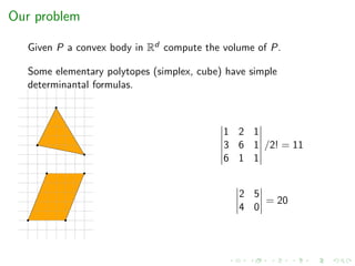
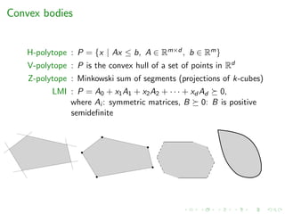
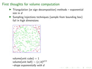
Download to read offline
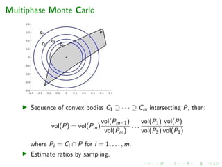
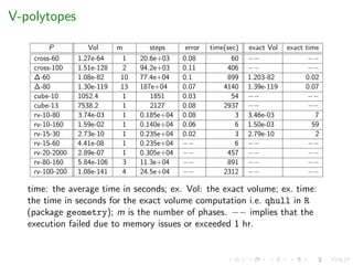
![Volume computation is hard!
#P-hard for V-, H-, Z-polytopes [DyerFrieze’88]
no deterministic poly-time algorithm can compute the volume
with less than exponential relative error (oracle
model) [Elekes’86]
open problem if V-polytope and H-polytope representations
available](https://image.slidesharecdn.com/kuleuven2020-200204132505/85/High-dimensional-sampling-and-volume-computation-6-320.jpg)
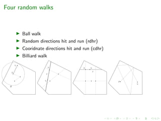
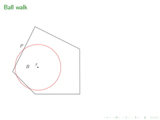
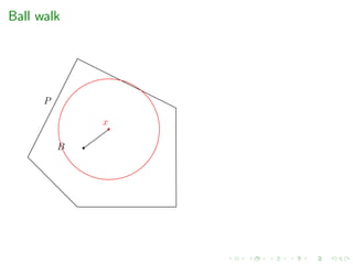
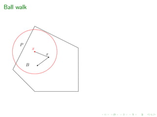
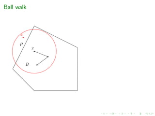
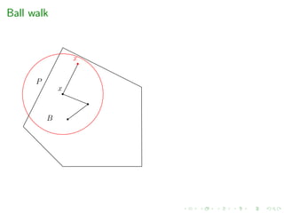
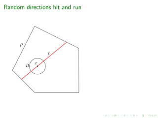
![Randomized algorithms
Volume algorithms parts
1. Multiphase Monte Carlo (MMC)
e.g. Sequence of balls, Annealing of functions
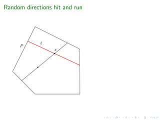
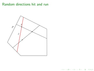
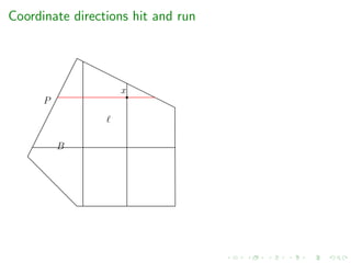
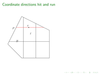
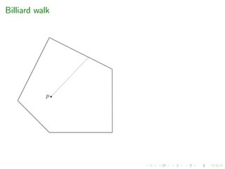
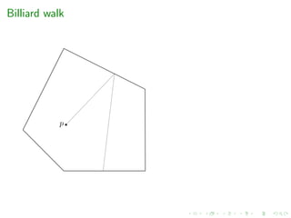
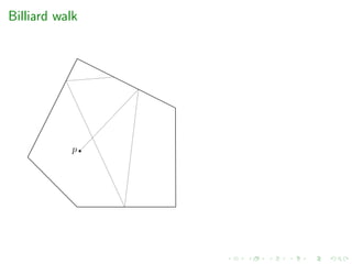
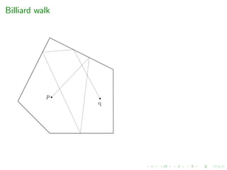
2. Sampling via geometric random walks
e.g. grid-walk, ball-walk, hit-and-run, billiard walk
Notes:
MMC (1) at each phase computes a ratio of integrals or
volumes via sampling (2)
geometric random walks are Markov chains where each ”event”
is a d-dimensional point
Algorithmic complexity is polynomial in d [Dyer, Frieze,
Kannan’91]](https://image.slidesharecdn.com/kuleuven2020-200204132505/85/High-dimensional-sampling-and-volume-computation-7-320.jpg)

![Complexity of random walks
Year & Authors Random walk Mixing time cost per step
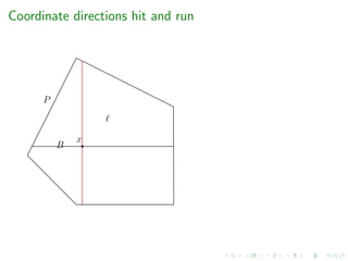
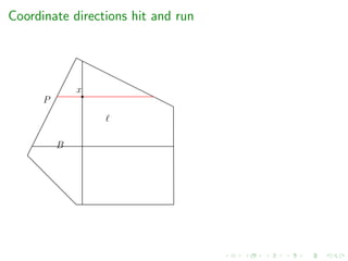
[Berbee et al.’87] Coordinate Hit-and-Run ?? O(m)
[Lovasz et al.’06] Hit-and-Run O∗(d3) O(md)
[Kannan et al.’09] Dikin walk O(md) O(md2)
[Polyak et al.’14] Billiard walk ?? O(mR + md)
[Lee et al.’16] Geodesic walk O(md3/4) O(md2)
[Lee et al.’17] Ball walk O∗(d2.5) O(md)
[Chen et al.’17] Vaidya walk O(m1/2d3/2) O(md2)
[Lee et al.’17] Riemmanian HMC O(md2/3) O(md2)
[Chevallier et al.’18] HMC with reflections ?? O(md)
[Mangoubi et al.’19] sublinear Ball walk O(d4.5) ∼ O(m)
Mixing times are unrealistically high for practical purposes
Billiard walk, CDHR and HMC with reflections seems the most
efficient in practice but there is not guarantee on the mixing
time](https://image.slidesharecdn.com/kuleuven2020-200204132505/85/High-dimensional-sampling-and-volume-computation-27-320.jpg)
![State-of-the-art
Theory:
Authors-Year Complexity Algorithm
(oracle steps)
[Dyer, Frieze, Kannan’91] O∗(d23) Seq. of balls + grid walk
[Kannan, Lovasz, Simonovits’97] O∗(d5) Seq. of balls + ball walk + isotropy
[Lovasz, Vempala’03] O∗(d4) Annealing + hit-and-run
[Cousins, Vempala’15] O∗(d3) Gaussian cooling (* well-rounded)
[Lee, Vempala’18] O∗(md
2
3 ) Hamiltonian walk (** H-polytopes)](https://image.slidesharecdn.com/kuleuven2020-200204132505/85/High-dimensional-sampling-and-volume-computation-28-320.jpg)
![State-of-the-art
Theory:
Authors-Year Complexity Algorithm
(oracle steps)
[Dyer, Frieze, Kannan’91] O∗(d23) Seq. of balls + grid walk
[Kannan, Lovasz, Simonovits’97] O∗(d5) Seq. of balls + ball walk + isotropy
[Lovasz, Vempala’03] O∗(d4) Annealing + hit-and-run
[Cousins, Vempala’15] O∗(d3) Gaussian cooling (* well-rounded)
[Lee, Vempala’18] O∗(md
2
3 ) Hamiltonian walk (** H-polytopes)
Software:
1. [Emiris, F’14] Sequence of balls + coordinate hit-and-run
2. [Cousins, Vempala’16] Gaussian cooling + hit-and-run
3. [Chalikis, Emiris, F’20] Convex body annealing + billiard walk](https://image.slidesharecdn.com/kuleuven2020-200204132505/85/High-dimensional-sampling-and-volume-computation-29-320.jpg)
![State-of-the-art
Theory:
Authors-Year Complexity Algorithm
(oracle steps)
[Dyer, Frieze, Kannan’91] O∗(d23) Seq. of balls + grid walk
[Kannan, Lovasz, Simonovits’97] O∗(d5) Seq. of balls + ball walk + isotropy
[Lovasz, Vempala’03] O∗(d4) Annealing + hit-and-run
[Cousins, Vempala’15] O∗(d3) Gaussian cooling (* well-rounded)
[Lee, Vempala’18] O∗(md
2
3 ) Hamiltonian walk (** H-polytopes)
Software:
1. [Emiris, F’14] Sequence of balls + coordinate hit-and-run
2. [Cousins, Vempala’16] Gaussian cooling + hit-and-run
3. [Chalikis, Emiris, F’20] Convex body annealing + billiard walk
Notes:
(2) is (theory + practice) faster than (1)
(1),(2) efficient only for H-polytopes
(3) efficient also for V-,Z-polytope, non-linear convex bodies
C++ implementation of (2) ×10 faster than original (MATLAB)](https://image.slidesharecdn.com/kuleuven2020-200204132505/85/High-dimensional-sampling-and-volume-computation-30-320.jpg)
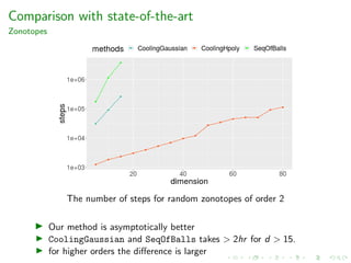
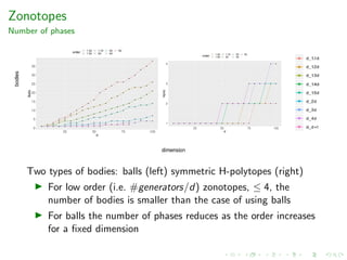
![Zonotopes
Performance
Experimental results for zonotopes.
z-d-k Body order Vol m steps time(sec)
z-5-500 Ball 100 4.63e+13 1 0.1250e+04 22
z-20-2000 Ball 100 2.79e+62 1 0.2000e+04 1428
z-50-65 Hpoly 1.3 1.42e+62 1 1.487e+04 173
z-50-75 Hpoly 1.5 2.96e+66 2 1.615e+04 253
z-100-150 Hpoly 1.5 2.32+149 3 15.43e+04 2992
z-60-180 Hpoly 3 8.71e+111 2 5.059e+04 417
z-100-200 Hpoly 3 5.27e+167 3 15.25e+04 2515
z-d-k: random zonotope in dimension d with k generators;
Body: the type of body used in MMC; m: number of bodies in
MMC
Used to evaluate zonotope approximation methods in
engineering [Kopetzki’17]](https://image.slidesharecdn.com/kuleuven2020-200204132505/85/High-dimensional-sampling-and-volume-computation-34-320.jpg)
![Applications
Biogeography & engineering
Volume of zonotopes is used to test methods for order
reduction which is important in several areas: autonomous
driving, human-robot collaboration and smart grids [Althoff et
al.]
Volumes of intersections of polytopes are used in bio-geography
to compute biodiversity and related measures e.g. [Barnagaud,
Kissling, Tsirogiannis, F, Villeger, Sekercioglu’17]](https://image.slidesharecdn.com/kuleuven2020-200204132505/85/High-dimensional-sampling-and-volume-computation-37-320.jpg)
![Applications
Combinatorics & Machine Learning
Volume can be used for counting linear extensions of a partially
ordered set. This arises in sorting [Peczarski 2004], sequence
analysis [Mannila et al.2000], convex rank tests [Morton et
al.2009], preference reasoning [Lukasiewicz et al.2014], partial
order plans [Muise et al.2016], learning graphical models
[Niinim¨aki et al. 2016] See also [Talvitie et al.AAAI’2018]
e.g. elements a, b, c
partial order a < c
3 linear extensions: abc, acb, bac](https://image.slidesharecdn.com/kuleuven2020-200204132505/85/High-dimensional-sampling-and-volume-computation-38-320.jpg)
![Applications
Computing integrals for AI
In Weighted Model Integration (WMI), given is a SMT formula
and a weight function, then we want to compute the weight of
the SMT formula.
e.g. SMT formula:
(A & (X > 20) | (X > 30)) & (X < 40)
Boolean formula + comparison operations. Let X has a weight
function of w(X) = X2 and w(A) = 0.3.
WMI answers the question of the weight of this formula i.e.
integration of a weight function over convex sets.
[P.Z.D. Martires et al.2019]](https://image.slidesharecdn.com/kuleuven2020-200204132505/85/High-dimensional-sampling-and-volume-computation-39-320.jpg)


This document discusses algorithms for computing the volume of high-dimensional convex bodies. It begins by introducing the problem and some challenges in high dimensions. It then describes various randomized algorithms that use sampling techniques like Markov chain Monte Carlo (MCMC) to estimate volumes. Specific algorithms discussed include multiphase Monte Carlo, hit-and-run sampling, and billiard walks. The document reviews the theoretical and practical complexity of these algorithms. It also presents applications of volume computation in fields like engineering, biology, and machine learning.