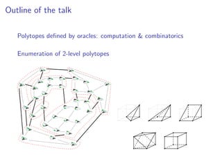
Download as PDF, PPTX

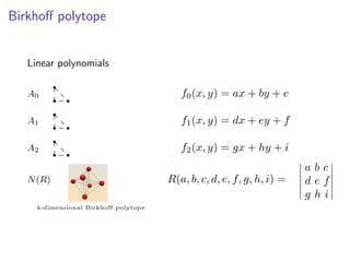
![Newton polytope
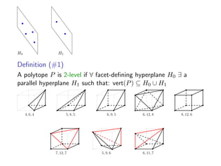
Definition
Given polynomial f ∈ K[x1, . . . , xn] the Newton polytope N(f) of
f is the convex hull of the support, i.e. exponent vectors of
monomials with non-zero coefficient.
3
2
1 2 3 5
5
f(x1, x2) = 8x2 + x1x2 − 24x2
2 −
16x2
1 + 220x2
1x2 − 34x1x2
2 −
84x3
1x2 +6x2
1x2
2 −8x1x3
2 +8x3
1x2
2 +
8x3
1 + 18x3
2
N(f)
1](https://image.slidesharecdn.com/lselunchtimeseminar15-200124133357/85/Polyhedral-computations-in-computational-algebraic-geometry-and-optimization-4-320.jpg)
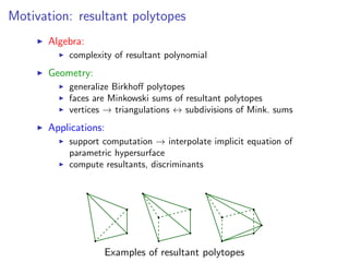
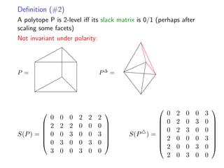
![Polytopes and Algebra
Definition
Given are polynomials f0, f1, . . . , fn ∈ K[x1, . . . , xn], s.t. the
supports define an essential family A0, A1, . . . , An ⊂ Zn, i.e. the
Ai generate Zn and any k-subset generates a sublattice of
dimension ≥ k.
The system’s (sparse) resultant R is the polynomial in the system’s
coefficients, defined up to sign, which vanishes iff the polynomials
have a common root in the corresponding toric variety X:
(K
∗
)n ⊂ X.
The resultant polytope N(R) is the Newton polytope of R.
A0
A1
N(R)R(a, b, c, d, e) = ad2
b + c2
b2
− 2caeb + a2
e2
f0(x) = ax2
+ b
f1(x) = cx2
+ dx + e](https://image.slidesharecdn.com/lselunchtimeseminar15-200124133357/85/Polyhedral-computations-in-computational-algebraic-geometry-and-optimization-5-320.jpg)
![Existing work
Resultants, secondary polytopes, Cayley trick [GKZ ’94]
TOPCOM [Rambau ’02] computes all vertices of secondary
polytope.
[Michiels & Verschelde DCG’99] coarse equivalence classes of
secondary polytope vertices.
[Michiels & Cools DCG’00] decomposition of Σ(A) in
Minkoski summands, including N(R).
Tropical geometry [Sturmfels-Yu ’08]: algorithms for resultant
polytope (GFan library) [Jensen-Yu ’11] and discriminant
polytope (TropLi software) [Rincn ’12].](https://image.slidesharecdn.com/lselunchtimeseminar15-200124133357/85/Polyhedral-computations-in-computational-algebraic-geometry-and-optimization-7-320.jpg)
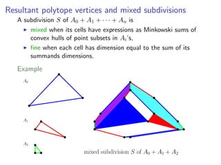
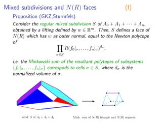
![Resultant polytope vertices and mixed subdivisions
A subdivision S of A0 + A1 + · · · + An is
mixed when its cells have expressions as Minkowski sums of
convex hulls of point subsets in Ai’s,
fine when each cell has dimension equal to the sum of its
summands dimensions.
Theorem [GKZ ’94, Sturmfels ’94]
many-to-one relation between regular fine mixed subdivisions
and N(R) vertices
one-to-one relation between regular fine mixed subdivisions
and secondary polytope Σ(A) vertices](https://image.slidesharecdn.com/lselunchtimeseminar15-200124133357/85/Polyhedral-computations-in-computational-algebraic-geometry-and-optimization-10-320.jpg)
![Combinatorics of resultant polytopes
[GKZ’90] Univariate case, general-dimensional N(R):
The Ai are multisets from Z: |A0| = k0 + 1, |A1| = k1 + 1 ⇒
⇒ dim N(R) = k0 + k1 − 1, k0+k1
k0
vertices, k0k1 + 3 facets.
[Sturmfels’94] Multivariate case / up to 3 dimensions
The only resultant polytopes up to dimension 3](https://image.slidesharecdn.com/lselunchtimeseminar15-200124133357/85/Polyhedral-computations-in-computational-algebraic-geometry-and-optimization-17-320.jpg)
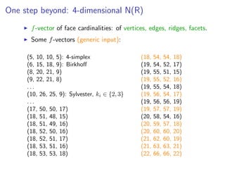
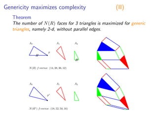
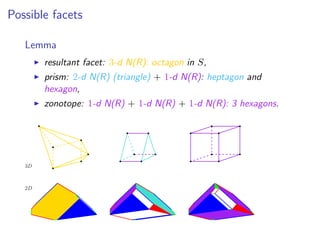
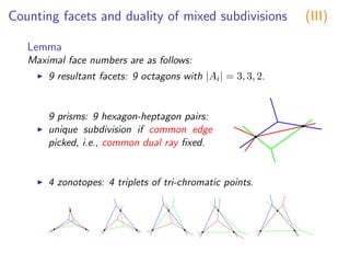
![Combinatorics of 4-dim resultant polytopes
Theorem (Dickenstein,Emiris,F)
Given essential family A0, A1, . . . , An ⊂ Zn, with N(R) of
dimension 4, N(R) is (a degeneration of) any of the following
polytopes:
(i) |Ai| : 2 . . . 2, 5, N(R) is the 4-simplex, f-vector (5, 10, 10, 5).
(ii) |Ai| : 2 . . . 2, 3, 4, N(R) f-vector (10, 26, 25, 9).
(iii) |Ai| : 2 . . . 2, 3, 3, 3, N(R) has maximal face numbers
˜f3 = 22, ˜f2 = 66, ˜f1 = ˜f0 + 44, and 22 ≤ ˜f0 ≤ 28.
Degenarations can only decrease the number of faces.
Previous upper bound for vertices yields 6608 [Sturmfels’94].
Focus on new case (iii): reduces to n = 2 and
|A0| = |A1| = |A2| = 3](https://image.slidesharecdn.com/lselunchtimeseminar15-200124133357/85/Polyhedral-computations-in-computational-algebraic-geometry-and-optimization-19-320.jpg)
![Extensions - Open problems
Algorithmic
Total polynomial algorithms for CH (edge-directions
[Emiris-F-Gartner])
Volume computation (randomized implementation [Emiris-F])
Lattice points enumeration
Combinatorial
The maximum f-vector of a 4d N(R) is (22, 66, 66, 22)
Explain symmetry of maximal f-vectors](https://image.slidesharecdn.com/lselunchtimeseminar15-200124133357/85/Polyhedral-computations-in-computational-algebraic-geometry-and-optimization-24-320.jpg)
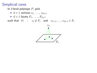
![Examples of 2-level polytopes
Birkhoff polytopes := convhull of permutation matrices
Hanner polytopes := iterated products / free sums of
segments
Stable set polytope STAB(G) with G perfect
Hansen polytopes := twisted prisms over STAB(G), G perfect
{x ∈ [0, 1]d | Ax = b} where A is totally unimodular and b
integer](https://image.slidesharecdn.com/lselunchtimeseminar15-200124133357/85/Polyhedral-computations-in-computational-algebraic-geometry-and-optimization-30-320.jpg)

![Embeddings
1 0 0 0 · · · 0 0
∗ 1 0 0 · · · 0 0
∗ ∗ 1 0 · · · 0 0
.
.
.
.
.
.
.
.
.
∗ ∗ ∗ ∗ · · · 1 0
∗ ∗ ∗ ∗ · · · ∗ 1
=
0
M
.
.
.
0
∗ · · · ∗ 1
Lemma
For 2L P an x-embedding has 0/1 facets:
P = {x ∈ Rd
| ∀E ∈ E : 0
i∈E
xi 1}
for some E with subsets of [d] and vert(P) ⊆ M−1{0, 1}d ⊆ Zd
(E contains all the subsets of [d] if P is the simplex)
Lemma
For 2L P a y-embedding is P = conv(X) for X ⊆ {0, 1}d
Remark: The two embeddings linked: y = Mx ⇐⇒ x = M−1y](https://image.slidesharecdn.com/lselunchtimeseminar15-200124133357/85/Polyhedral-computations-in-computational-algebraic-geometry-and-optimization-37-320.jpg)
![A proxy for 2LP: closed sets
Definition
I := M−1 · {0, 1}d then A ⊆ I is closed if clI(A) = A.
E(A) :=
x∈A
{E ⊆ [d] | 0 ≤ x(E) ≤ 1} .
clI(A) := {x ∈ I | 0 ≤ x(E) ≤ 1 for every E ∈ E(A)} .
Lemma
If 2L P in x-embedding then the vertex set of P is a closed set wrt
M−1 · {0, 1}d.](https://image.slidesharecdn.com/lselunchtimeseminar15-200124133357/85/Polyhedral-computations-in-computational-algebraic-geometry-and-optimization-38-320.jpg)
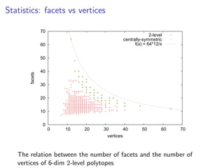
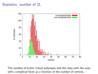
![Experimental results
d 2L ∆-f STAB polar CS Birk 0/1 closed sets
3 5 4 4 4 2 4 8 19
4 19 12 11 12 4 11 192 350
5 106 41 33 42 13 33 1,048,576 21239
6 1150 248 148 276 45 129 ∼ 1.8 · 1019
1.05 · 108
7 - - 906 - 238 661 - -
8 - - 8887 - - 4530 - -
Combinatorially equivalent 0/1 polytopes and 2L polytopes
∆-f: with on simplicial facet
STAB: stable sets of perfect graphs [Hougardy06]
polar: 2-level polytopes whose polar is 2-level
CS: centrally symmetric
Birk: Birkhoff polytope faces [Paffenholz13]
’-’: exact numbers are unknown.](https://image.slidesharecdn.com/lselunchtimeseminar15-200124133357/85/Polyhedral-computations-in-computational-algebraic-geometry-and-optimization-40-320.jpg)
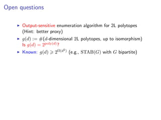
![Open questions
Output-sensitive enumeration algorithm for 2L polytopes
(Hint: better proxy)
g(d) := #(d-dimensional 2L polytopes, up to isomorphism)
Is g(d) = 2poly(d)?
Known: g(d) 2Ω(d2) (e.g., STAB(G) with G bipartite)
xc(P) = extension complexity = min # facets of a lift of P
f(d) := max{xc(P) | P is d-dimensional 2L polytope}
Is f(d) = 2polylog(d)? (“log-rank conj. for slack matrices”)
xc(STAB(G)) 2O(log2
n)
for n-vertex perfect G (Yannakakis’91)
f(d) 2
˜O(
√
d) for d-dimensional 2LP (Lovett ’14)
g(d) 2O[poly(d)f2(d)] (Rothvoss ’11)](https://image.slidesharecdn.com/lselunchtimeseminar15-200124133357/85/Polyhedral-computations-in-computational-algebraic-geometry-and-optimization-44-320.jpg)

The document summarizes a talk on polyhedral computations in computational algebraic geometry and optimization. It discusses algorithms for enumerating vertices of resultant polytopes and 2-level polytopes. Applications include support computation for implicit equations and computing resultants and discriminants. Open problems include finding the maximum number of faces of 4-dimensional resultant polytopes and explaining symmetries in their maximal f-vectors.